Transition State Theory for dissipative systems without a dividing surface

Abstract

Transition State Theory is a central cornerstone in reaction dynamics. Its key step is the identification of a dividing surface that is crossed only once by all reactive trajectories. This assumption is often badly violated, especially when the reactive system is coupled to an environment. The calculations made in this way then overestimate the reaction rate and the results depend critically on the choice of the dividing surface. In this Letter, we study the phase space of a stochastically driven system close to an energetic barrier in order to identify the geometric structure unambiguously determining the reactive trajectories, which is then incorporated in a simple rate formula for reactions in condensed phase that is both independent of the dividing surface and exact.

Transition State Theory (TST) provides the conceptual framework for a large part of reaction rate theory. Originally developed to describe reactivity of small molecules Truhlar, Hase, and Hynes (1983); Truhlar, Garrett, and Klippenstein (1996); Miller (1998), it was later extended to study a wide variety of processes in very different fields that only have in common the existence of a transition from well-defined “reactant” to “product” states Toller et al. (1985); Eckhardt (1995); Jaffé, Farrelly, and Uzer (2000); Koon et al. (2000); Jaffé et al. (2002); Uzer et al. (2002); Komatsuzaki and Berry (2002); Waalkens, Burbanks, and Wiggins (2004a, b). Its great success comes from its simplicity, since it gives a straightforward answer to the two central problems in chemical dynamics: the identification of the reaction mechanism and a simple approximation to the reaction rate.

The rate limiting step in many reactions is the crossing of an energetic barrier, the top of which forms a bottleneck that the system must cross as the reaction takes place. If a dividing surface (DS) is placed close to this bottleneck, reaction rates can be readily computed from the steady-state flux through it. The TST approximation is obtained under the assumption that the reactive classical trajectories cross the DS only once and never return. Very often, for example when the system is strongly coupled to a noisy environment such as a liquid solvent, this no-recrossing assumption fails, and any conventional DS is crossed many times by a typical trajectory. As a result, TST calculations significantly overestimate reaction rates, and considerable effort has been devoted to the construction of a DS that minimizes recrossing Truhlar, Garrett, and Klippenstein (1996). The problem mainly derives from the fact that this special surface plays a double role: It defines (or separates) reactant and product regions, and it also serves to identify the reactive trajectories. To the latter purpose the DS is ill suited. Despite this fundamental drawback, TST remains attractive since reactive trajectories are simply identified as those crossing the DS. This criterion only takes into account the instantaneous velocity at the DS, without requiring any time consuming trajectory simulation.

Important advances in TST have recently been achieved within the approach of modern nonlinear dynamics: A strictly recrossing free DS can be constructed in the phase space of reactive systems with arbitrarily many degrees of freedom Uzer et al. (2002); Waalkens, Burbanks, and Wiggins (2004a, b). These results were generalized to systems interacting with an environment Bartsch, Hernandez, and Uzer (2005); Bartsch, Uzer, and Hernandez (2005); Bartsch et al. (2006, 2008); Hernandez, Uzer, and Bartsch (2010); Kawai and Komatsuzaki (2010a, b). It has been shown that the desired exact TST can be constructed, in the harmonic limit, by using a moving DS only crossed once by the reactive trajectories Bartsch, Hernandez, and Uzer (2005); Bartsch, Uzer, and Hernandez (2005). Accurate results are still obtained for moderate anharmonicities Bartsch et al. (2006) and can be improved by normal form calculations Kawai and Komatsuzaki (2010a, b).

In this Letter, we make a step forward by presenting an explicit description of geometric phase space structures in an anharmonic noisy system and an analytical scheme that relies on these structures for the computation of exact TST reaction rates for arbitrary multidimensional potentials coupled to a noisy environment. The key point is the demonstration that reactive trajectories can be rigorously identified solely from their initial conditions, thus avoiding the choice of a (arbitrary) DS. This is done in terms of the stable manifold associated to a “noisy” Transition State (TS) trajectory jiggling in phase space. This geometric structure encodes the relevant information about the noise in the most economical manner and it can easily be incorporated into a rate calculation. Our method retains the fundamental simplicity of TST, also providing the conceptual tools to develop new computational algorithms. An application to the simple case of the one-dimensional quartic potential is presented as an illustration.

The Langevin equation (LE) has been widely used to model the interaction of a reactive system with a surrounding heat bath Hänggi, Talkner, and Borkovec (1990); Pechukas (1976); Chandler (1978). Being a classical model, this description neglects quantum effects such as barrier tunnelling, which can be important in the case of light particles Bothma, Gilmore, and McKenzie (2010), and the interaction with excited surfaces through conical intersections Polli and et al. (2010).

The dynamics of a unit mass particle defined by coordinate $x$ moving in a one-dimensional potential $U(x)$ is given by

$$\ddot{x}=-U^{\prime}(x)-\gamma\dot{x}+\xi_{\alpha}(t).$$ (1)

Here, $\xi_{\alpha}(t)$ is the fluctuating force exerted by the bath, which is connected to the damping strength, $\gamma$, by the fluctuation–dissipation theorem

$$\left\langle\xi_{\alpha}(t)\xi_{\alpha}(t^{\prime})\right\rangle_{\alpha}=2k_{\text{B}}T\gamma\,\delta(t-t^{\prime}).$$ (2)

The model potential that we have chosen to study is

$$U(x)=-\frac{1}{2}\omega_{\text{b}}^{2}x^{2}+\frac{c_{4}}{4}x^{4},$$ (3)

although our derivation equally applies to any other one-dimensional case. This generality will be emphasized by using $f(t)$, equal to $-c_{4}x^{3}$ in our case, to denote any anharmonic force. The extension to higher dimension is straightforward and will be presented elsewhere.

For every fixed realization of the noise, the LE gives rise to a specific trajectory called TS trajectory Bartsch, Hernandez, and Uzer (2005); Bartsch, Uzer, and Hernandez (2005). This orbit remains in the vicinity of the energetic barrier for all times, without ever descending into any of the potential wells. Other trajectories will be referred to the TS trajectory, which will be taken as a moving coordinate origin. Since the LE is a second order differential equation, its phase space is two-dimensional, with coordinates $x$ and $v=\dot{x}$. If we now introduce the new coordinates

$$u =\frac{v-\lambda_{\text{s}}x}{\lambda_{\text{u}}-\lambda_{\text{s}}}, s =\frac{-v+\lambda_{\text{u}}x}{\lambda_{\text{u}}-\lambda_{\text{s}}},$$ (4)

with

$$\lambda_{\text{u,s}}=\tfrac{1}{2}[-\gamma\pm(\gamma^{2}+4\omega_{\text{b}}^{2})^{1/2}],$$ (5)

relative values are defined by the time-dependent shift

$$\Delta u=u-u^{\ddagger}_{\alpha}(t),\qquad\Delta s=s-s^{\ddagger}_{\alpha}(t),$$ (6)

where the coordinates of the TS-trajectory are

$$u^{\ddagger}_{\alpha}(t) =-\frac{1}{\lambda_{\text{u}}-\lambda_{\text{s}}}\,\int_{t}^{\infty}\xi_{\alpha}(\tau)\,e^{\lambda_{\text{u}}(t-\tau)}\,d\tau,$$

$$s^{\ddagger}_{\alpha}(t) =-\frac{1}{\lambda_{\text{u}}-\lambda_{\text{s}}}\,\int_{-\infty}^{t}\xi_{\alpha}(\tau)\,e^{\lambda_{\text{s}}(t-\tau)}\,d\tau.$$ (7)

The corresponding equations of motion are

$$\Delta\dot{u} =\lambda_{\text{u}}\Delta u+\frac{f(x^{\ddagger}_{\alpha}+\Delta u+\Delta s)}{\lambda_{\text{u}}-\lambda_{\text{s}}},$$ (8a)

$$\Delta\dot{s} =\lambda_{\text{s}}\Delta s-\frac{f(x^{\ddagger}_{\alpha}+\Delta u+\Delta s)}{\lambda_{\text{u}}-\lambda_{\text{s}}},$$ (8b)

with $x^{\ddagger}_{\alpha}(t)$=$u^{\ddagger}_{\alpha}(t)$+$s^{\ddagger}_{\alpha}(t)$ [and $v^{\ddagger}_{\alpha}(t)$=$\lambda_{\text{u}}u^{\ddagger}_{\alpha}(t)$+$\lambda_{\text{s}}s^{\ddagger}_{\alpha}(t)$]. Now, the geometric phase space structure in the vicinity of the barrier can be easily discussed. First, in the harmonic limit, i.e. $f(x)=0$, the equations of motion (8) are trivially solved, giving

$$\Delta u(t) =\Delta u(0)\,e^{\lambda_{\text{u}}t}, \qquad\Delta s(t) =\Delta s(0)\,e^{\lambda_{\text{s}}t}.$$ (9)

Since $\lambda_{\text{u}}>0$ and $\lambda_{\text{s}}<0$, $\Delta u$ increases exponentially in time, whereas $\Delta s$ shrinks accordingly. More importantly, the lines $\Delta u=0$ and $\Delta s=0$ are invariant under the dynamics of the system; being the unstable and stable manifolds of the origin, respectively. As shown in Fig. 1(a), these invariant manifolds separate trajectories with different qualitative behavior: Those above the stable manifold (larger relative velocity) move to the product side in the distant future, while those below it move, on the other hand, towards the reactant side.

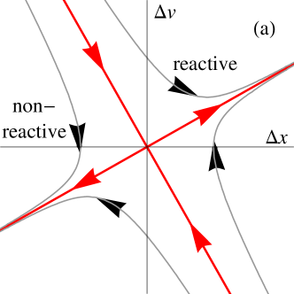
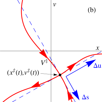
Figure 1: (color online) Schematic view of the phase space structure near the Transition State trajectory for the Langevin equation for the harmonic (a) and anharmonic (b) cases. The time-dependent invariant manifolds are attached to the TS trajectory, and move through phase space with it. In the harmonic limit they appear as (red) straight lines (a), but they get deformed by anharmonic couplings (b). Reactive and non-reactive trajectories are represented in black.

In space fixed coordinates the invariant manifolds appear attached to the TS trajectory, as shown by the dashed lines in Fig. 1(b); their instantaneous position depends on the realization of the noise. Accordingly, the manifolds move through phase space but they still separate trajectories with different asymptotic behaviors. The stable manifold intersects the $x=0$ axis in a point with velocity $V^{\ddagger}_{\alpha}$. Trajectories with initial position $x=0$ and initial velocity $v$ larger than this critical velocity, $V^{\ddagger}_{\alpha}$, are reactive, while trajectories with initial velocities $v<V^{\ddagger}_{\alpha}$ are not. The (random) value $V^{\ddagger}_{\alpha}$ therefore encodes the relevant information about the realization of the noise concisely. In other words, once the instantaneous position of the stable manifold is known, any trajectory can unambiguously be classified from the values of its initial condition as reactive or non-reactive. Finally, the presence of anharmonicities ($f(x)\neq 0$) will distort the invariant manifolds, as indicated by the red lines with arrows in Fig. 1(b). The main step of the theory to be developed here is the calculation of this deformation.

This critical velocity can be calculated from the condition that the trajectory with $x(0)=0$ and $v(0)=V^{\ddagger}_{\alpha}$ is contained in the stable manifold of the TS trajectory. To find this trajectory, which will be called critical trajectory, we formally solve the equations of motion (8) by

$$\Delta u(t)=C_{u}\,e^{\lambda_{\text{u}}t}+\frac{S[\lambda_{\text{u}},f(x^{\ddagger}+\Delta u+\Delta s);t]}{\lambda_{\text{u}}-\lambda_{\text{s}}},$$ (10a)

$$\Delta s(t)=C_{s}\,e^{\lambda_{\text{s}}t}-\frac{S[\lambda_{\text{s}},f(x^{\ddagger}+\Delta u+\Delta s);t]}{\lambda_{\text{u}}-\lambda_{\text{s}}},$$ (10b)

where $C_{u}$ and $C_{s}$ are two arbitrary constants, and the integral operator

$$S_{\tau}[\mu,g;t]=\begin{cases}\displaystyle-\int_{t}^{\infty}g(\tau)\,\exp[\mu(t-\tau)]\,d\tau\!\!\!&:\;\operatorname{Re}\mu>0,\\[12.91663pt] \displaystyle+\int_{0}^{t}g(\tau)\,\exp[\mu(t-\tau)]\,d\tau\!\!\!&:\;\operatorname{Re}\mu<0.\end{cases}$$ (11)

has been introduced as a convenient shorthand notation. The subscript $\tau$ indicating the integration variable in Eq. (11) will be left out whenever this does not cause any ambiguity. The unknown constants $C_{u}$ and $C_{s}$ can be determined by noticing that the critical trajectory should approach the TS trajectory for large times. In particular, it should remain bounded for $t\to\infty$. This can only be satisfied if $C_{u}=0$. [This condition also ensures that the $S$ functional in Eq. (10a) is well defined.] With this choice, Eq. (10a) determines the initial condition $\Delta u(0)$, and $C_{s}=\Delta s(0)$ can then be found from the condition that $x(0)=x^{\ddagger}_{\alpha}(0)+\Delta u(0)+\Delta s(0)=0$. Finally, the coordinate transformation (4) yields

$$V^{\ddagger}_{\alpha}=v(0)=(\lambda_{\text{u}}-\lambda_{\text{s}})u(0)$$ (12)

In general, Eq. (10) represents only a formal solution, since its right-hand side depends on the unknown functions $\Delta u$ and $\Delta s$. However, since it is known that the critical trajectory remains in the neighborhood of the barrier at all times, the anharmonic force will be small, and then its influence can be evaluated through perturbation theory, thus obtaining an expansion $V_{\alpha}^{\ddagger}=V_{0}^{\ddagger}+c_{4}V_{1}^{\ddagger}+c_{4}^{2}V_{2}^{\ddagger}+\dots$ in powers of the anharmonic coupling parameter $c_{4}$.

In the harmonic approximation the critical trajectory is given by

$$\Delta u_{0}(t)=0\qquad\text{and}\qquad\Delta s_{0}(t)=-x^{\ddagger}(0)e^{\lambda_{\text{s}}t},$$ (13)

and for this case Eq. (12) yields

$$V_{\alpha}^{\ddagger}\equiv V^{\ddagger}_{0}=(\lambda_{\text{u}}-\lambda_{\text{s}})u^{\ddagger}(0)$$

that was already derived in Ref. Bartsch et al., 2008. When the solution (13) is substituted into Eq. (10), $x=x^{\ddagger}+\Delta u+\Delta s$ is replaced by

$$X_{\alpha}(t)=x_{\alpha}^{\ddagger}(t)-e^{\lambda_{\text{s}}t}x_{\alpha}^{\ddagger}(0),$$ (14)

which is the harmonic approximation to the coordinate $x(t)$ of the critical trajectory. Equation (10a) then gives

$$\Delta u_{1}(t)=\frac{1}{\lambda_{\text{u}}-\lambda_{\text{s}}}S[\lambda_{\text{u}},f(X);t],$$

and therefore the leading-order velocity correction is

$$V^{\ddagger}_{1}=S[\lambda_{\text{u}},f(X);0]=-c_{4}S[\lambda_{\text{u}},X_{\alpha}^{3};0]$$ (15)

for the quartic potential (3). Given the initial condition $\Delta s_{1}(0)=x^{\ddagger}_{\alpha}(0)-\Delta u_{1}(0)$, $\Delta s_{1}(t)$ can be obtained from Eq. (10b), and then substituted into Eq. (10a) to find $\Delta u_{2}(t)$. In this way, the second-order velocity correction

$$V^{\ddagger}_{2}=-\frac{3c_{4}^{2}}{\lambda_{\text{u}}-\lambda_{\text{s}}}S_{\tau}\Big{[}\lambda_{\text{u}},X^{2}(\tau)\left(e^{\lambda_{\text{s}}\tau}S[\lambda_{\text{u}},X^{3};0]\right.\\ \left.-S[\lambda_{\text{u}},X^{3};\tau]+\bar{S}[\lambda_{\text{s}},X^{3};\tau]\right);0\Big{]}$$ (16)

is obtained. In Fig. 2 we present a comparison between numerical (exact) results for the critical velocity, $V_{\alpha}^{\ddagger}$, for one realization of the noise and the approximate values computed using (15) and (16), as a function of the anharmonic parameter, $c_{4}$.

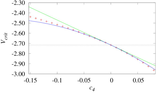
Figure 2: Critical velocity for one realization of the noise as a function of the anharmonicity for $\omega_{\text{b}}=1$, $\gamma=2.5$, and $k_{\text{B}}T=1$: Numerical simulation results (red crosses), harmonic approximation (gray line), perturbative results to first-order (green straight line), and second-order (blue line).

In order to calculate the corresponding reaction rate, $k$, we choose the simplest DS, defined by $x=0$, and use the basic flux-over-population rate formula (see e.g. Hänggi, Talkner, and Borkovec (1990)), which states that $k$ is proportional to the reactive flux

$$J=\left\langle v\right\rangle^{\text{react}}_{\alpha,v}$$ (17)

across the DS. This flux is to be averaged over different realizations of the noise, $\alpha$, and also over a Boltzmann ensemble of initial velocities, $v$, for trajectories starting at the DS. Notice that only reactive trajectories should be included in the average.

The non-recrossing assumption of conventional TST can be restated here by saying that the reactive trajectories are those crossing the DS with velocity $v>0$. We call the rate constant obtained with this approximation $k^{\text{TST}}$. Any effects beyond TST are customarily summarized Hänggi, Talkner, and Borkovec (1990) into a transmission coefficient $\kappa=k/k^{\text{TST}}$.

In terms of our stochastic invariant manifolds, reactive trajectories are characterized by $v>V^{\ddagger}_{\alpha}$, as discussed before. Using this criterion, the Boltzmann average over velocities in Eq. (17) can be evaluated, as it was in Ref. Bartsch et al., 2008 for the harmonic case. This gives the exact expression

$$\kappa=\left\langle\exp\left(-\frac{V_{\alpha}^{{\ddagger}2}}{2k_{\text{B}}T}\right)\right\rangle_{\alpha},$$ (18)

where only the average over the noise remains to be done. By substituting the perturbative expansion for the critical velocity into this expression and expanding the exponential, a perturbative series of rate corrections, $\kappa=\kappa_{0}+c_{4}\kappa_{1}+c_{4}^{2}\kappa_{2}+\dots$, is obtained, where

$$\kappa_{0} =\left\langle E\right\rangle_{\alpha},$$ (19a)

$$\kappa_{1} =-\frac{1}{k_{\text{B}}T}\left\langle EV_{0}^{\ddagger}V_{1}^{\ddagger}\right\rangle_{\alpha},$$ (19b)

with the abbreviated notation

$$E=\exp\left(-\frac{V_{0}^{{\ddagger}2}}{2k_{\text{B}}T}\right)=\exp\left[-\frac{(\lambda_{\text{u}}-\lambda_{\text{s}})^{2}\,u_{\alpha}^{{\ddagger}2}(0)}{2k_{\text{B}}T}\right].$$ (20)

Expressions similar to (19) can be obtained for the higher-order corrections. The leading order $\kappa_{0}$ was evaluated in Ref. Bartsch et al., 2008. It yields the well-known Kramers result for the transmission factor. With the result (15), the first correction term is given by

$$\kappa_{1}=\frac{c_{4}(\lambda_{\text{u}}-\lambda_{\text{s}})}{k_{\text{B}}T}\,S_{\tau}\left[\lambda_{\text{u}},\left\langle E\,u_{\alpha}^{\ddagger}(0)X_{\alpha}^{3}(\tau)\right\rangle_{\alpha};0\right].$$ (21)

To perform the remaining average and subsequently evaluate the $S$ functional, note that $u^{\ddagger}_{\alpha}(t)$ and $s^{\ddagger}_{\alpha}(t)$, and consequently $X_{\alpha}(t)$, are Gaussian random processes, whose correlation functions were given in Bartsch, Uzer, and Hernandez, 2005. Details of this calculation are irrelevant for the purpose of this Letter and will be presented elsewhere. The final result is given by

$$\kappa_{1}=-\frac{3}{4}\frac{c_{4}\,k_{\text{B}}T}{\omega_{\text{b}}^{4}}\,\mu\left(\frac{1-\mu^{2}}{1+\mu^{2}}\right)^{2}$$ (22)

in terms of the dimensionless parameter $\mu=\lambda_{\text{u}}/\omega_{\text{b}}$. This expression agrees with the corrections given in Refs. Pollak and Talkner, 1993; Talkner and Pollak, 1993; Talkner, 1994. A comparison between perturbation theory and the results of a numerical simulation is shown in Fig. 3, along with the second-order perturbative correction, which can be obtained in a similar manner. The perturbative results describe the rate correctly as long as the coupling is not too strong. For large negative values of $c_{4}$ the second-order correction loses its accuracy. By contrast, it is accurate for all positive $c_{4}$ shown in the figure. If $c_{4}$ is increased further, the wells of the model potential (3) become too shallow for a rate theory to be meaningful.

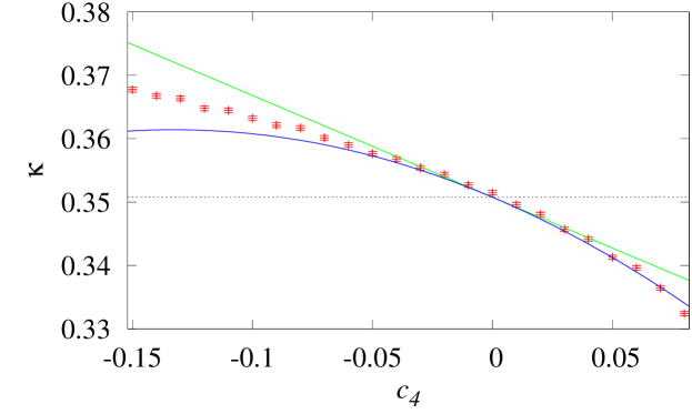
Figure 3: Transmission factor as a function of the anharmonicity for the same values and legend of Fig. 2.

In summary, we have demonstrated that the use of stochastic invariant structures allows a rigorous TST reaction rate calculation in general anharmonic and noisy systems. In our approach, the DS is only used to define reactant and product regions. To identify reactive trajectories we employ the stable manifold that is determined by the dynamics of the system itself. The resulting rate formula (18) is not only remarkably compact, but also exact. In particular, the arbitrariness that is usually introduced by the choice of a DS is absent. Although our presentation is based on an analytical perturbation expansion, the method can easily be incorporated into a numerical scheme to achieve an efficient rate calculation in complex systems.

Support from MICINN–Spain under Contracts nrs. MTM2009–14621 and i–MATH CSD2006–32 is gratefully acknowledged. FR thanks UPM for a doctoral fellowship and the hospitality of the members of the School of Mathematics at Loughborough University, where part of this work was done.

References

- Truhlar, Hase, and Hynes (1983) D. G. Truhlar, W. L. Hase, and J. T. Hynes, J. Phys. Chem. 87, 2664 (1983).
- Truhlar, Garrett, and Klippenstein (1996) D. G. Truhlar, B. C. Garrett, and S. J. Klippenstein, J. Phys. Chem. 100, 12771 (1996).
- Miller (1998) W. H. Miller, Faraday Discuss. Chem. Soc. 110, 1 (1998).
- Toller et al. (1985) M. Toller, G. Jacucci, G. DeLorenzi, and C. P. Flynn, Phys. Rev. B 32, 2082 (1985).
- Eckhardt (1995) B. Eckhardt, J. Phys. A 28, 3469 (1995).
- Jaffé, Farrelly, and Uzer (2000) C. Jaffé, D. Farrelly, and T. Uzer, Phys. Rev. Lett. 84, 610 (2000).
- Koon et al. (2000) W. S. Koon, M. W. Lo, J. E. Marsden, and S. D. Ross, Chaos 10, 427 (2000).
- Jaffé et al. (2002) C. Jaffé, S. D. Ross, M. W. Lo, J. Marsden, D. Farrelly, and T. Uzer, Phys. Rev. Lett. 89, 011101 (2002).
- Uzer et al. (2002) T. Uzer, C. Jaffé, J. Palacián, P. Yanguas, and S. Wiggins, Nonlinearity 15, 957 (2002).
- Komatsuzaki and Berry (2002) T. Komatsuzaki and R. S. Berry, Adv. Chem. Phys. 123, 79 (2002).
- Waalkens, Burbanks, and Wiggins (2004a) H. Waalkens, A. Burbanks, and S. Wiggins, J. Phys. A 37, L257 (2004a).
- Waalkens, Burbanks, and Wiggins (2004b) H. Waalkens, A. Burbanks, and S. Wiggins, J. Chem. Phys. 121, 6207 (2004b).
- Bartsch, Hernandez, and Uzer (2005) T. Bartsch, R. Hernandez, and T. Uzer, Phys. Rev. Lett. 95, 058301 (2005).
- Bartsch, Uzer, and Hernandez (2005) T. Bartsch, T. Uzer, and R. Hernandez, J. Chem. Phys. 123, 204102 (2005).
- Bartsch et al. (2006) T. Bartsch, T. Uzer, J. M. Moix, and R. Hernandez, J. Chem. Phys. 124, 244310 (2006).
- Bartsch et al. (2008) T. Bartsch, T. Uzer, J. M. Moix, and R. Hernandez, J. Phys. Chem. B 112, 206 (2008).
- Hernandez, Uzer, and Bartsch (2010) R. Hernandez, T. Uzer, and T. Bartsch, Chem. Phys. 370, 270 (2010).
- Kawai and Komatsuzaki (2010a) S. Kawai and T. Komatsuzaki, PCCP 12, 7626 (2010a).
- Kawai and Komatsuzaki (2010b) S. Kawai and T. Komatsuzaki, PCCP 12, 7636 (2010b).
- Hänggi, Talkner, and Borkovec (1990) P. Hänggi, P. Talkner, and M. Borkovec, Rev. Mod. Phys. 62, 251 (1990).
- Pechukas (1976) P. Pechukas, in Dynamics of Molecular Collisions, Part B, edited by W. H. Miller (Plenum, New York, 1976).
- Chandler (1978) D. Chandler, J. Chem. Phys. 68, 2959 (1978).
- Bothma, Gilmore, and McKenzie (2010) J. P. Bothma, J. B. Gilmore, and R. H. McKenzie, New J. Phys. 12, 055002 (2010).
- Polli and et al. (2010) D. Polli et al., Nature 467, 440 (2010).
- Pollak and Talkner (1993) E. Pollak and P. Talkner, Phys. Rev. E 47, 922 (1993).
- Talkner and Pollak (1993) P. Talkner and E. Pollak, Phys. Rev. E 47, R21 (1993).
- Talkner (1994) P. Talkner, Chem. Phys. 180, 199 (1994).