Abstract

Multivariate spatial field data are increasingly common and whose modeling typically relies on building cross-covariance functions to describe cross-process relationships. An alternative viewpoint is to model the matrix of spectral measures. We develop the notions of coherence, phase and gain for multidimensional stationary processes. Coherence, as a function of frequency, can be seen to be a measure of linear relationship between two spatial processes at that frequency band. We use the coherence function to illustrate fundamental limitations on a number of previously proposed constructions for multivariate processes, suggesting these options are not viable for real data. We also give natural interpretations to cross-covariance parameters of the Matérn class, where the smoothness indexes dependence at low frequencies while the range parameter can imply dependence at low or high frequencies. Estimation follows from smoothed multivariate periodogram matrices. We illustrate the estimation and interpretation of these functions on two datasets, forecast and reanalysis sea level pressure and geopotential heights over the equatorial region. Examining these functions lends insight that would otherwise be difficult to detect and model using standard cross-covariance formulations.

Keywords: coherency; gain; multivariate random field; periodogram; phase; reanalysis; squared coherence; spectral density

1 Introduction

The theory of univariate continuous stochastic processes has become well developed over nearly a century of research. The past quarter century or so has seen an increasing interest and development of models for multivariate spatial processes. The recent review by Genton and Kleiber (2015) gives a relatively comprehensive treatment of the basic approaches that have been explored to build stochastic spatial models. In the discussion, Bevilacqua et al. (2015) pose the question, given the recent deluge of multivariate constructions, “which parametric model is more flexible?” Indeed, the relative strengths and weaknesses of multivariate models have been explored only empirically, that is, by testing a battery of different models on particular datasets, and comparing performance either by likelihood values or by predictive cross-validation (in the multivariate context, spatial prediction is known as co-kriging). Thus, a fundamental open question is: (1) to what extent can the flexibilities of model constructions be compared theoretically? Additionally, most models are motivated in the covariance domain, and the natural follow-up question is: (2) are there other approaches than covariance to measure and quantify spatial dependence?

We introduce the notion of spectral coherence, phase and gain for multidimensional and multivariate spatial random fields. We propose that these functions allow for natural partial answers to the critical open questions (1) and (2). We show that a number of previously proposed models lack sufficient practical flexibility in terms of prediction, and we suggest insights into well established models such as the multivariate Matérn, where parameters such as the cross-covariance smoothness and range have had elusive direct interpretations that relate to process behavior.

Let us illustrate the ideas developed in this manuscript by considering the time series case first. Suppose $Z_{i}(t),i=1,2$ is a bivariate complex-valued weakly stationary time series on $t\in\mathbb{R}$ with covariance functions ${\rm Cov}(Z_{k}(t+h),Z_{k}(t))=C_{kk}(h)$ and cross-covariance functions ${\rm Cov}(Z_{k}(t+h),Z_{\ell}(t))=C_{k\ell}(t)$ for $k\not=\ell$. The corresponding spectral densities are $f_{k\ell}(\omega)=(2\pi)^{-1}\int_{\mathbb{R}}C_{k\ell}(h)\exp(-i\omega h){\rm d}h$ for $\omega\in\mathbb{R}$. Spectral modeling in time series is well developed; for example, traditional autoregressive moving average models imply processes with rational spectral densities. The function

$$\gamma(\omega)^{2}=\frac{|f_{12}(\omega)|^{2}}{f_{11}(\omega)f_{22}(\omega)}$$

is known as the squared coherence function, and can be interpreted as a quantification of the linear relationship between $Z_{1}(t)$ and $Z_{2}(t)$ at frequency $\omega$ (Brockwell and Davis, 2009).

We entertain two example datasets from the atmospheric sciences. Both are reforecast and reanalysis data products over the equatorial region based on a well established numerical weather prediction (NWP) model. Reanalysis forecasts are from a fixed version of a NWP model that are run retrospectively to generate a large database of model forecasts and analyses (in this context, an analysis can be considered a best estimate of the current state of the atmosphere). First we look at forecasted surfaces of sea level pressure at daily forecast horizons between 24 and 192 hours. We show that coherence can be used as a diagnostic to assess forecast quality, and additionally illustrate frequency bands at which forecasts improve over time. The second dataset involves geopotential heights at differing pressure levels. We show that coherence and phase extract and highlight qualities of the spatial relationship between different pressure levels that are difficult to model using extant multivariate covariance constructions, and indeed illustrate some fundamental limitations of existing popular constructions.

2 Spectra for Multivariate Random Fields

Suppose $\mathbf{Z}(\mathbf{s})=(Z_{1}(\mathbf{s}),\ldots,Z_{p}(\mathbf{s}))^{\rm T}\in\mathbb{C}^{p}$ is a $p$-variate weakly stationary random field on $\mathbf{s}\in\mathbb{R}^{d}$ admitting a matrix-valued covariance function $\mathbf{C}(\mathbf{h})=(C_{ij}(\mathbf{h}))_{i,j=1}^{p}$ where $C_{ij}(\mathbf{h})={\rm Cov}(Z_{i}(\mathbf{s}+\mathbf{h}),Z_{j}(\mathbf{s}))$. For simplicity of exposition we suppose $\mathbf{Z}(\mathbf{s})$ is a mean zero process. For complex-valued stationary processes, ${\rm Cov}(Z_{i}(\mathbf{s}_{1}),Z_{j}(\mathbf{s}_{2}))=\mathbb{E}(Z_{i}(\mathbf{s}_{1})\overline{Z_{j}(\mathbf{s}_{2})})$, so that $C_{ij}(\mathbf{h})=\overline{C_{ji}(\mathbf{h})}$. The main obstacle to multivariate process modeling is developing flexible classes of matrix-valued covariance functions $\mathbf{C}$ that are nonnegative definite. We say $\mathbf{C}$ is nonnegative definite if, for any choices of $a_{ik}\in\mathbb{C}$ and locations $\mathbf{s}_{k}\in\mathbb{R}^{d}$ for $i=1,\ldots,p$ and $k=1,\ldots,n$ we have

$$\sum_{i=1}^{p}\sum_{j=1}^{p}\sum_{k=1}^{n}\sum_{\ell=1}^{n}a_{ik}\overline{a_{j\ell}}C_{ij}(\mathbf{s}_{k},\mathbf{s}_{\ell})\geq 0.$$

Note this reduces to the usual definition of nonnegative definiteness for a univariate covariance, $p=1$.

For univariate processes, Bochner’s Theorem states that $C_{ii}(\mathbf{h})$ is a valid (i.e., nonnegative definite) function if and only if it can be written

$$C(\mathbf{h})=\int_{\mathbb{R}^{d}}\exp(i\boldsymbol{\omega}^{\rm T}\mathbf{h}){\rm d}F(\boldsymbol{\omega})$$

where $F$ is a positive finite measure (Stein, 1999). If $F$ admits a density $f$ with respect to the Lebesgue measure on $\mathbb{R}^{d}$, we call it the spectral density for $C$. The multivariate extension of Bochner’s fundamental result is given by Cramér (1940), and is contained in the following theorem specialized to covariances admitting spectral densities.

Theorem 1 (Cramér 1940).

A matrix-valued function $\mathbf{C}:\mathbb{R}^{d}\to\mathbb{C}^{p\times p},\mathbf{C}=(C_{ij})_{i,j=1}^{p}$ is nonnegative definite if and only if

$$C_{ij}(\mathbf{h})=\int_{\mathbb{R}^{d}}\exp(i\boldsymbol{\omega}^{\rm T}\mathbf{h})f_{ij}(\boldsymbol{\omega}){\rm d}\boldsymbol{\omega}$$

for $i,j=1,\ldots,p$ such that the matrix $\mathbf{f}(\boldsymbol{\omega})=(f_{ij}(\boldsymbol{\omega}))_{i,j=1}^{p}$ is nonnegative definite for all $\boldsymbol{\omega}\in\mathbb{R}^{d}$.

The functions $f_{ij}(\boldsymbol{\omega})$ are the spectral and cross-spectral densities for the marginal and cross-covariance functions $C_{ij}(\mathbf{h})$. Note that $f_{ij}(\boldsymbol{\omega})=\overline{f_{ji}(\boldsymbol{\omega})}$. When the spectral density exists, it can be solved for as the Fourier transform of the covariance function,

$$f_{ij}(\boldsymbol{\omega})=\frac{1}{(2\pi)^{d}}\int_{\mathbb{R}^{d}}\exp(-i\boldsymbol{\omega}^{\rm T}\mathbf{h})C_{ij}(\mathbf{h}){\rm d}\mathbf{h}.$$

Theorem 1 has primarily been used in practice to build multivariate covariance models, by specifying matrices of spectral densities that are nonnegative definite for all frequencies.

2.1 Coherence

In time series, the notion of frequency coherence is well developed, and can be used, for instance, to assess whether one time series is related to another by a time invariant linear filter. These notions carry over to the spatial case, and form the point of entry for our analyses.

If $C_{ij}(\mathbf{h}),i,j=1,2$ form a matrix-valued covariance function with associated spectral densities $f_{ij}(\boldsymbol{\omega})$, then define the coherence function (or coherency function)

$$\gamma(\boldsymbol{\omega})=\frac{f_{12}(\boldsymbol{\omega})}{\sqrt{f_{11}(\boldsymbol{\omega})f_{22}(\boldsymbol{\omega})}}.$$

We might assume $f_{ii}(\boldsymbol{\omega})>0$ for all $\boldsymbol{\omega}\in\mathbb{R}^{d}$ for $i=1,2$, but can define $\gamma(\boldsymbol{\omega})=0$ if $f_{ii}(\boldsymbol{\omega})=0$. The coherence function can be complex-valued, so in practice we examine the absolute coherence function, $|\gamma(\boldsymbol{\omega})|$. The real-valued function $|\gamma(\boldsymbol{\omega})|^{2}$ is the squared coherence function, and by Theorem 1, $0\leq|\gamma(\boldsymbol{\omega})|^{2}\leq 1$ for all $\boldsymbol{\omega}$. Values of $|\gamma(\boldsymbol{\omega})|$ near unity indicate a linear relationship between $Z_{1}(\mathbf{s})$ and $Z_{2}(\mathbf{s})$ at particular frequency bands.

The following theorem relates the coherence to optimal prediction of a random process based on another process. The predictive estimator is based on a kernel smoothed process which is a natural predictor given the interpretation of the univariate kriging weights as a kernel function (Kleiber and Nychka, 2015).

Theorem 2.

Suppose $(Z_{1}(\mathbf{s}),Z_{2}(\mathbf{s}))^{\rm T}$ is a complex-valued mean zero weakly stationary bivariate field with matrix-valued covariance $\mathbf{C}(\mathbf{h})$ admitting a spectral density matrix $\mathbf{f}(\boldsymbol{\omega})=(f_{ij}(\boldsymbol{\omega}))_{i,j=1}^{2}$ that is everywhere nonzero. Then the continuous square integrable function $K(\mathbf{u}):\mathbb{R}^{d}\to\mathbb{C}$ that minimizes $\mathbb{E}\big{|}Z_{1}(\mathbf{s}_{0})-\int_{\mathbb{R}^{d}}K(\mathbf{u}-\mathbf{s}_{0})Z_{2}(\mathbf{u}){\rm d}\mathbf{u}\big{|}^{2}$ is

$$K(\mathbf{u})=\frac{1}{(2\pi)^{d}}\int_{\mathbb{R}^{d}}\exp(-i\boldsymbol{\omega}^{\rm T}\mathbf{u})\frac{f_{12}(\boldsymbol{\omega})}{f_{22}(\boldsymbol{\omega})}{\rm d}\boldsymbol{\omega}=\frac{1}{(2\pi)^{d}}\int_{\mathbb{R}^{d}}\exp(-i\boldsymbol{\omega}^{\rm T}\mathbf{u})\sqrt{\frac{f_{11}(\boldsymbol{\omega})}{f_{22}(\boldsymbol{\omega})}}\gamma(\boldsymbol{\omega}){\rm d}\boldsymbol{\omega}.$$ (1)

Additionally, the spectral density of the predictor $\hat{Z}_{1}(\mathbf{s}_{0})=\int_{\mathbb{R}^{d}}K(\mathbf{u}-\mathbf{s}_{0})Z_{2}(\mathbf{u}){\rm d}\mathbf{u}$ is

$$f_{1|2}(\boldsymbol{\omega})=f_{11}(\boldsymbol{\omega})|\gamma(\boldsymbol{\omega})|^{2}$$ (2)

for all $\boldsymbol{\omega}\in\mathbb{R}^{d}$.

In particular, the relationship (1) implies that the optimal weighting function is modulated by the coherence between the two processes, and indeed has greater spectral weight on frequencies with high coherence. An immediate corollary to Theorem 2 is

$$|\gamma(\boldsymbol{\omega})|^{2}=\frac{f_{1|2}(\boldsymbol{\omega})}{f_{11}(\boldsymbol{\omega})}.$$

Thus, the coherence has an attractive interpretation as the amount of variability that can be attributed to a linear relationship between two processes at a particular frequency. In the following development, we use the coherence function to illuminate fundamental limitations on some popular multivariate covariance constructions.

The coherence function can be used as a tool to compare proposed multivariate models, as an indicator of the amount of flexibility of bivariate relationships at differing frequencies. For example, a rather classic approach to specifying covariances is separability, setting $\mathbf{C}(\mathbf{h})=\mathbf{R}C(\mathbf{h})$ where $C(\mathbf{h})$ is a univariate covariance function and $\mathbf{R}$ is a $p\times p$ positive definite matrix (Mardia and Goodall, 1993; Helterbrand and Cressie, 1994; Bhat et al., 2010). This approach has been empirically shown to be insufficiently flexible, and the following lemma contributes to the empirical results.

Lemma 3.

If $\mathbf{C}(\mathbf{h})=\mathbf{R}C(\mathbf{h})$ where $C:\mathbb{R}^{d}\to\mathbb{R}$ is a covariance function and $\mathbf{R}$ is a $p\times p$ positive definite matrix with $(i,j)$th entry $r_{ij}$, then the squared coherence between the $i$th and $j$th process is constant, in particular $\gamma_{ij}(\boldsymbol{\omega})^{2}=(r_{ij}r_{ji})/(r_{ii}r_{jj})$.

A more sophisticated method of generating multivariate covariance structures is to convolve univariate square integrable functions (Gaspari and Cohn, 1999; Oliver, 2003; Gaspari et al., 2006; Majumdar and Gelfand, 2007). In particular, if $c_{i}:\mathbb{R}^{d}\to\mathbb{R}$ are square integrable functions for $i=1,\ldots,p$ then $C_{ij}(\mathbf{h})=(c_{i}\star c_{j})(\mathbf{h})$ is a valid matrix-covariance function where $\star$ denotes the convolution operator. This is sometimes known as covariance convolution (especially when $c_{i}$ are positive definite functions to begin with). The following proposition suggests this approach to model building is overly-restrictive, and indeed implies that the resulting coherence is necessarily constant over all frequencies.

Proposition 4.

If $c_{1}$ and $c_{2}$ are square integrable functions on $\mathbb{R}^{d}$ and a matrix-valued covariance is defined via $C_{ij}=c_{i}\star c_{j}$ for $i,j=1,2$ where $\star$ denotes convolution, then $\gamma(\boldsymbol{\omega})\equiv 1$ for all $\boldsymbol{\omega}\in\mathbb{R}^{d}$ such that the Fourier transforms of $c_{i}$ and $c_{j}$ are nonzero.

Multivariate processes can sometimes be modeled as being related by local averaging. For example, the relationship between column integrated ozone observations and local ozone might be plausibly modeled as observations being locally averaged over the true underlying field (Cressie and Johannesson, 2008). Wind observations are often time averaged over moving windows to produce smoother and more stable observation series (Hering et al., 2015). The following proposition characterizes the coherence in such situations, and serves to illustrate the intimate link between process relationship and coherence.

Proposition 5.

If $Z_{1}(\mathbf{s})$ is a weakly stationary stochastic process and $Z_{2}(\mathbf{s})=\int_{\mathbb{R}^{d}}K(\mathbf{u}-\mathbf{s})Z_{1}(\mathbf{u}){\rm d}\mathbf{u}$ for some continuous square integrable kernel function $K:\mathbb{R}^{d}\to\mathbb{R}$ that is symmetric, then $\gamma(\boldsymbol{\omega})\equiv 1$ for all $\boldsymbol{\omega}\in\mathbb{R}^{d}$ such that the Fourier transform of $K$ is nonzero.

According to Proposition 5, estimated coherences near unity over all frequency bands may be indicative of a linear or local averaged relationship between processes, and this result may serve as the theoretical basis for testing such a hypothesis. Fuentes (2006) uses a similar notion to develop a test for separability of space-time processes.

The kernel convolution method, introduced by Ver Hoef and Barry (1998) and Ver Hoef et al. (2004), originally involved representing a process as a moving average against a white noise process. In simple cases this yields the covariance convolution model. This can be generalized to

$$Z_{k}(\mathbf{s})=\int_{\mathbb{R}^{d}}g_{k}(\mathbf{x}-\mathbf{s})W(\mathbf{x}){\rm d}\mathbf{x}$$ (3)

where $W(\mathbf{x})$ is a mean zero stationary process with covariance $C(\mathbf{h})$, and $g_{k}:\mathbb{R}^{d}\to\mathbb{R}$ are square integrable symmetric kernel functions for $k=1,\ldots,p$. As with each previous construction, this approach also yields constant coherence.

Proposition 6.

If $Z_{1}(\mathbf{s})$ and $Z_{2}(\mathbf{s})$ are constructed as in (3), then $\gamma(\boldsymbol{\omega})$ is constant for all $\boldsymbol{\omega}\in\mathbb{R}^{d}$.

For all of these models, separable, covariance convolution and kernel convolution, the resulting multivariate structure is restricted to constant coherence. In light of Theorem 2, this suggests that none of these models can attain optimal prediction for any multivariate processes exhibiting nontrivial coherences. Indeed the examples below in Section 4 exhibit nonconstant coherence, and call for more flexible modeling frameworks.

2.2 Phase and Gain

Similar notions to frequency coherence can be motivated by examining spectral density matrices. If $(Z_{1}(\mathbf{s}),Z_{2}(\mathbf{s}))^{\rm T}$ is a stationary random vector with spectral density matrix $(f_{ij}(\boldsymbol{\omega}))_{i,j=1}^{2}$ then define $A(\boldsymbol{\omega})=f_{12}(\boldsymbol{\omega})/f_{11}(\boldsymbol{\omega})$. Note that $A(\boldsymbol{\omega})$ is possibly complex-valued. We define the gain function $G(\boldsymbol{\omega})=|A(\boldsymbol{\omega})|$ which is sometimes referred to as the gain of $Z_{2}(\mathbf{s})$ on $Z_{1}(\mathbf{s})$ in time series (Brockwell and Davis, 2009). Additionally define the phase function at frequency $\boldsymbol{\omega}$ as $\phi(\boldsymbol{\omega})=\arg A(\boldsymbol{\omega})$, the complex argument of $A(\boldsymbol{\omega})$. Note that the phase function satisfies $\phi(\boldsymbol{\omega})\in(-\pi,\pi]$ and $\phi(-\boldsymbol{\omega})=-\phi(\boldsymbol{\omega})$.

The interpretations of gain and phase are most clear when considering processes built by the relationship $Z_{1}(\mathbf{s})=\alpha Z_{2}(\mathbf{s}-\mathbf{u})$ for some $\mathbf{u}\in\mathbb{R}^{d}$ and $\alpha\not=0$, i.e., $Z_{1}$ is a shifted and rescaled version of $Z_{2}$. Then it is straightforward to show that the phase function is

$$\phi(\boldsymbol{\omega})=\begin{cases}-\boldsymbol{\omega}^{\rm T}\mathbf{u}\,(\mod 2\pi),&\alpha>0\\ \pi-\boldsymbol{\omega}^{\rm T}\mathbf{u}\,(\mod 2\pi)&\alpha<0.\end{cases}$$

Li and Zhang (2011) develop an approach to modeling this type of asymmetric cross-covariance behavior. This result shows that their construction will have phase shift function that depends on the angle $\boldsymbol{\omega}^{\rm T}\mathbf{u}$. This result may be used as an exploratory data approach or as the basis for a statistical test to suggest whether a pair of spatial processes exhibit an asymmetric relationship; Li and Zhang (2011) use the empirical cross-correlation function to visually assess such asymmetric behavior. The gain function in this case is simply $G(\boldsymbol{\omega})=|\alpha|$; all frequency components of $Z_{2}$ are exaggerated by an amount $\alpha$ for $Z_{1}$.

Below we consider some multivariate constructions that are particular to real-valued processes having real-valued spectral matrices. Any model with real-valued cross-spectral density has $\phi(\boldsymbol{\omega})\equiv 0$, but a possibly non-trivial gain function. Thus, testing for $\phi(\boldsymbol{\omega})\equiv 0$ can be viewed as a test for a real-valued cross-spectral density, which seems very relevant given most multivariate models are developed under this assumption.

2.3 Revisiting the Multivariate Matérn

The multivariate Matérn is a model for matrix-valued covariance functions such that each process is marginally described by a Matérn covariance function, and all cross-covariance functions also fall in the Matérn class (Gneiting et al., 2010; Apanasovich et al., 2012). Specifically, the multivariate Matérn imposes $C_{ii}(\mathbf{h})=\sigma_{i}^{2}{\rm M}(\mathbf{h}\,|\,\nu_{i},a_{i})$ for $i=j$ and $C_{ij}(\mathbf{h})=\rho_{ij}\sigma_{i}\sigma_{j}{\rm M}(\mathbf{h}\,|\,\nu_{ij},a_{ij})$ for $1\leq i\not=j\leq p$. Here, ${\rm M}(\mathbf{h}\,|\,\nu,a)=(2^{1-\nu}/\Gamma(\nu))(a\|\mathbf{h}\|)^{\nu}{\rm K}_{\nu}(a\|\mathbf{h}\|)$ where $K_{\nu}$ is a modified Bessel function of the second kind of order $\nu$. Gneiting et al. (2010) and Apanasovich et al. (2012) discuss restrictions on the parameters $\nu_{i},a_{i},\nu_{ij},a_{ij}$ and $\rho_{ij}$ that result in a valid model.

The Matérn class is popular due to the smoothness parameters $\nu>0$ which continuously index smoothnesses of the sample paths of the process. In particular, sample paths are $m$ times differentiable if and only if $\nu>m$, and there is an additional relationship between $\nu$ and the fractal dimension in that sample paths have dimension $\max(d,d+1-\nu)$ (Goff and Jordan, 1988; Handcock and Stein, 1993). These interpretations and implications also hold in the multivariate case, where $\nu_{i}$ indexes the smoothness of the $i$th component process $Z_{i}(\mathbf{s})$. The parameters $a_{i}$ act as range parameters, and control the rate of decay of spatial correlation away from the origin.

A standing issue with the multivariate Matérn is that the cross-covariance parameters, $\nu_{ij}$ and $a_{ij}$ for $i\not=j$, do not have straightforward interpretations that are analogous to the marginal smoothness and range interpretations, and indeed nowhere in the literature have these parameters been linked directly to process behavior. We find that these parameters have direct interpretations when considering the coherence function between two processes.

The coherence function for a bivariate process with multivariate Matérn correlation is

$$\gamma(\boldsymbol{\omega})^{2}=\rho^{2}\frac{\Gamma(\nu_{12}+d/2)^{2}\Gamma(\nu_{1})\Gamma(\nu_{2})}{\Gamma(\nu_{1}+d/2)\Gamma(\nu_{2}+d/2)\Gamma(\nu_{12})^{2}}\frac{a_{12}^{4\nu_{12}}}{a_{1}^{2\nu_{1}}a_{2}^{2\nu_{2}}}\frac{(a_{1}^{2}+\|\boldsymbol{\omega}\|^{2})^{\nu_{1}+d/2}(a_{2}^{2}+\|\boldsymbol{\omega}\|^{2})^{\nu_{2}+d/2}}{(a_{12}^{2}+\|\boldsymbol{\omega}\|^{2})^{2\nu_{12}+d}}.$$

We explore in detail two simplified versions of this coherency function. First, consider the case where $a_{1}=a_{2}=a_{12}=a$, all covariance and cross-covariance functions share a common range. Then

$$\gamma(\boldsymbol{\omega})^{2}=\rho^{2}\frac{\Gamma(\nu_{12}+d/2)^{2}\Gamma(\nu_{1})\Gamma(\nu_{2})}{\Gamma(\nu_{1}+d/2)\Gamma(\nu_{2}+d/2)\Gamma(\nu_{12})^{2}}(a+\|\boldsymbol{\omega}\|^{2})^{\nu_{1}+\nu_{2}-2\nu_{12}}.$$ (4)

Figure 1: Coherence functions for various bivariate Matérns with $a_{11}=a_{12}=a_{22}=1,\nu_{11}=\nu_{22}=0.5$, varying $\nu_{12}$ and $\rho$.

The multivariate Matérn is a valid model only if $\nu_{12}\geq(\nu_{1}+\nu_{2})/2$, and thus by inspecting (4) we note some modeling implications resulting from these restrictions. First, if $\nu_{12}=(\nu_{1}+\nu_{2})/2$, the coherency is constant across all frequencies, implying a constant linear relationship between two processes at all frequency bands. Second, if $\nu_{12}>(\nu_{1}+\nu_{2})/2$, we have greater coherency at low frequencies, with $\gamma(\boldsymbol{\omega})\to 0$ as $\|\boldsymbol{\omega}\|\to\infty$. This analysis seems to suggest a natural interpretation of the cross-covariance smoothness in that it controls the amount of cross-process dependence at various frequencies, but can only imply greater or equal coherence at low frequencies versus high frequencies. Figure 1 serves to illustrate these points, showing various coherence functions for common length scale parameters $a_{11}=a_{12}=a_{22}=1$, varying $\nu_{12}$ and $\rho$.

Perhaps surprisingly, a similar analysis suggests the cross-covariance range parameter $a_{12}$ induces potentially greater flexibility in the coherence function than the smoothness parameter $\nu_{12}$. In particular, if $\nu_{1}=\nu_{2}=\nu_{12}=\nu$, the coherence function is

$$\gamma(\boldsymbol{\omega})^{2}=\rho^{2}\left(\frac{a_{12}^{2}}{a_{1}a_{2}}\right)^{2\nu}\left(\frac{(a_{1}^{2}+\|\boldsymbol{\omega}\|^{2})(a_{2}^{2}+\|\boldsymbol{\omega}\|^{2})}{(a_{12}^{2}+\|\boldsymbol{\omega}\|^{2})^{2}}\right)^{\nu+d/2}.$$ (5)

Examining (5), we see that, depending on whether $a_{12}\leq\min(a_{1},a_{2})$ or $a_{12}\geq\max(a_{1},a_{2})$ the coherence will have distinct behavior. For simplicity, set $a_{1}=a_{2}=a$. If $a_{12}<a$, the coherence will be greater for small frequencies than high frequencies, similar to the behavior implied by (4) when $\nu_{12}>(\nu_{1}+\nu_{2})/2$. However, here $\gamma(\boldsymbol{\omega})\to\rho a_{12}^{2\nu}/(a_{1}a_{2})^{\nu}$ as $\|\boldsymbol{\omega}\|\to\infty$, implying non-negligible coherence between processes at high frequencies, unlike that in (4). If $a_{12}>a$, we have the complementary result that $\gamma(\boldsymbol{\omega}_{1})<\gamma(\boldsymbol{\omega}_{2})$ for $\|\boldsymbol{\omega}_{1}\|<\|\boldsymbol{\omega}_{2}\|$, that is, two processes share behavior at high frequencies rather than low. Figure 2 illustrates these scenarios, and seems to suggest that, at least as far as coherence is concerned, the cross-covariance range parameter yields potentially greater flexibility than the cross-smoothness.

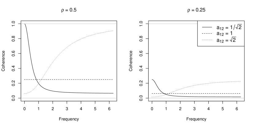
Figure 2: Coherence functions for various bivariate Matérns with $\nu_{11}=\nu_{12}=\nu_{22}=1,a_{11}=a_{22}=1$, varying $a_{12}$ and $\rho$.

The so-called parsimonious Matérn model is defined by imposing common range parameters as well as $\nu_{12}=(\nu_{1}+\nu_{2})/2$ (Gneiting et al., 2010). This model has been empirically shown to produce inferior model fits to datasets as compared to more general versions of the multivariate Matérn as well as other multivariate classes (Gneiting et al., 2010; Apanasovich et al., 2012). The coherence function for a bivariate parsimonious Matérn model is constant, $\gamma(\boldsymbol{\omega})=\rho$, which suggests an inflexible model for the spectral behavior of spatial processes.

We close this section with an empirical illustration of the implications of cross-covariance parameter choice on random field realizations and the associated low and high frequency behavior. We simulate two bivariate Matérn models on an equally-spaced grid of $256\times 256$ in $[0,8]^{2}$. In both cases we low-pass and high-pass filter the resulting bivariate field. The low-pass filter is a matrix of zeros except for a $3\times 3$ grid of $1/9$, while the high-pass filter is similar with a $3\times 3$ grid of $-1/9$ on the edge and $8/9$ in the center. The effect of the filters is to remove high frequency behavior (low-pass filtering) or low frequency behavior (high-pass filtering).

Figure 3 shows low-pass filtered realizations of two bivariate Gaussian processes with bivariate Matérn covariances. The top row is the case with equal ranges $a_{11}=a_{12}=a_{22}=1$ but with a greater cross-smoothness $\nu_{11}=\nu_{22}=0.5,\nu_{12}=1$. According to Figure 1, we should expect the realizations to show similar low frequency behavior, but dissimilar high frequency behavior. Indeed, panels (a) and (b) show similar low frequency behavior, while the pairwise scatterplot of high-passed values, panel (c), suggests little correlation at high frequencies. Complementary, the second row is the case with equal smoothnesses, $\nu_{11}=\nu_{12}=\nu_{21}=1$ but a greater cross-range parameter, $a_{11}=a_{22}=1,a_{12}=\sqrt{2}$. Figure 2 suggest we should expect less coherence at low frequencies while having greater correlation at high frequencies. Again, these theoretical results are reinforced: panels (d) and (e) are not suggestive of strong low frequency coherence, while panel (f) exhibits positively correlated high frequency characteristics (and indeed has an empirical correlation coefficient of approximately $0.25$).

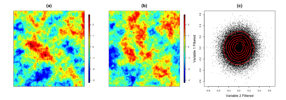
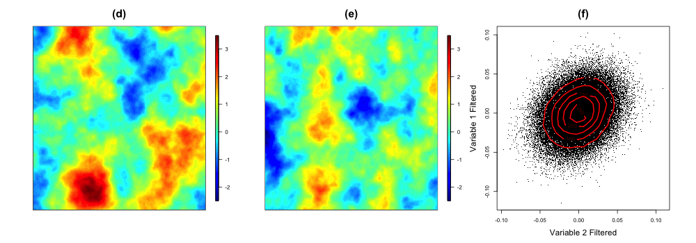
Figure 3: Low-pass filtered bivariate Matérn with $a_{11}=a_{12}=a_{22}=1,\nu_{11}=\nu_{22}=0.5,\nu_{12}=1$ and $\rho=0.5$ for the (a) first process, (b) second process. Panel (c) is the pairwise scatterplot of high-pass filtered values of the two processes with contour levels for comparison. Panels (d), (e) and (f) are analogous plots for a bivariate Matérn simulation with $\nu_{11}=\nu_{12}=\nu_{22}=1,a_{11}=a_{22}=1,a_{12}=\sqrt{2}$ and $\rho=0.5$.

2.4 The Linear Model of Coregionalization

The linear model of coregionalization (LMC) is a competing framework for multivariate modeling, and is built by decomposing a multivariate process as linear combinations of uncorrelated, univariate processes (Goulard and Voltz, 1992; Royle and Berliner, 1999; Wackernagel, 2003; Schmidt and Gelfand, 2003). In particular, we entertain the following version,

$$\mathbf{Z}(\mathbf{s})=\left(\begin{array}[]{c}Z_{1}(\mathbf{s})\\ Z_{2}(\mathbf{s})\end{array}\right)=\left(\begin{array}[]{cc}b_{11}&b_{12}\\ b_{21}&b_{22}\end{array}\right)\left(\begin{array}[]{c}W_{1}(\mathbf{s})\\ W_{2}(\mathbf{s})\end{array}\right)=\mathbf{B}\mathbf{W}(\mathbf{s})$$ (12)

The matrix $\mathbf{B}$ is known as the coregionalization matrix, and controls the strength of dependencies on the latent uncorrelated processes $\mathbf{W}$. For the following, suppose $W_{1}(\mathbf{s})$ and $W_{2}(\mathbf{s})$ are uncorrelated processes with spectral densities $f_{1}(\boldsymbol{\omega})$ and $f_{2}(\boldsymbol{\omega})$, respectively.

Given the number of parameters in the LMC, it is often useful to impose restrictions on the coregionalization matrix $\mathbf{B}$, such as setting $b_{11}=b_{22}=1$ (Berrocal et al., 2010). The following Lemma is the unsurprising result that the LMC yields multivariate processes that are exactly coherent when the coregionalization matrix has zero determinant.

Lemma 7.

In the linear model of coregionalization (12), if $b_{11}=b_{22}=1$ then the coherence function between $Z_{1}(\mathbf{s})$ and $Z_{2}(\mathbf{s})$ is unity if and only if $b_{12}b_{21}=1$.

Note that this result simply states that, under the LMC, two processes are exactly coherent when they differ only by a scalar multiplier.

Under the same working assumptions, $b_{11}=b_{22}=1$, we have the gain function of $Z_{2}(\mathbf{s})$ on $Z_{1}(\mathbf{s})$ is

$$G(\boldsymbol{\omega})=\frac{b_{21}f_{1}(\boldsymbol{\omega})+b_{12}f_{2}(\boldsymbol{\omega})}{f_{1}(\boldsymbol{\omega})+b_{12}^{2}f_{2}(\boldsymbol{\omega})}.$$

If, as is common in using the LMC, we set $b_{12}=0$, we have the gain function is simply $b_{21}$; that is, there is constant gain at all frequencies by the amount of coregionalization, $b_{21}$. The complementary case where $b_{21}=0$ yields the gain

$$G(\boldsymbol{\omega})=\frac{b_{12}f_{2}(\boldsymbol{\omega})}{f_{1}(\boldsymbol{\omega})+b_{12}^{2}f_{2}(\boldsymbol{\omega})},$$

that is, the relative contribution of component $b_{12}W_{2}(\mathbf{s})$ to the combined spectrum of $Z_{1}(\mathbf{s})$. As mentioned previously, if the latent processes have real-valued spectral densities, the phase function is exactly zero at all frequencies.

3 Estimation of Spectra

Suppose $\mathbf{Z}(\mathbf{s})$ is a $p$-variate process that has been observed at a regular grid of points $\{\mathbf{s}_{i}\}_{i=1}^{N}$, of marginal dimensions $n_{i},i=1,\ldots,d$ where $N=\prod_{i=1}^{d}n_{i}$. If grid spacing in the $i$th dimension is $\delta_{i}$, define $\delta=\prod_{i=1}^{d}\delta_{i}$. Then the spatial periodogram matrix with $(k,\ell)$th entry is defined as $\mathbf{I}(\boldsymbol{\omega})=(I_{k\ell}(\boldsymbol{\omega}))_{k,\ell=1}^{p}$ where

$$I_{k\ell}(\boldsymbol{\omega})=\frac{\delta}{(2\pi)^{p}N}\left(\sum_{k=1}^{N}Z_{k}(\mathbf{s}_{k})\exp(-i\mathbf{s}_{k}^{\rm T}\boldsymbol{\omega})\right)\overline{\left(\sum_{k=1}^{N}Z_{\ell}(\mathbf{s}_{k})\exp(-i\mathbf{s}_{k}^{\rm T}\boldsymbol{\omega})\right)}$$ (13)

is available at Fourier frequencies $\boldsymbol{\omega}=2\pi\mathbf{f}$ where $\mathbf{f}=(f_{1}/(\delta_{1}n_{1}),\ldots,f_{d}/(\delta_{d}n_{d}))^{\rm T}$ for $f_{i}\in\{-\lfloor(n_{i}-1)/2\rfloor,\ldots,n_{i}-\lfloor n_{i}/2\rfloor\}$. Note that $I_{k\ell}(\boldsymbol{\omega})=\overline{I_{\ell k}(\boldsymbol{\omega})}$.

Whereas in the time series literature it is natural to consider asymptotics as time $t\to\infty$, resulting in effectively uncorrelated blocks of a process, in the spatial realm there are two competing asymptotic frameworks. Increasing domain asymptotics is similar to the time series case where samples are taken on an ever-increasing domain in all axial directions, and typically asymptotic results here echo those in time series. The complementary version is infill asymptotics (sometimes called fixed-domain asymptotics) in which the domain boundary is fixed and points are sampled at an ever finer resolution within the domain (Zhang and Zimmerman, 2005). Depending on the asymptotic framework under consideration, the large sample properties of the periodogram (13) change.

Using infill asymptotics, Lim and Stein (2008) show that the raw multivariate periodogram can exhibit bias at low frequencies, and suggest prewhitening the process to overcome this inadequacy (in the univariate case Stein (1995) gives a simulated example where the bias is quite substantial). However, under a mixture of infill and increasing domain asymptotics, Fuentes (2002) showed (for univariate processes) the analogous result to the time series case that the periodogram is asymptotically unbiased and is uncorrelated at differing Fourier frequencies. Additionally, in this latter case it is not a consistent estimator, but must be smoothed to gain consistency.

Analogous to the time series and univariate spatial field case, under certain assumptions the nonparametric periodogram (13) is asymptotically unbiased, and generates asymptotically uncorrelated random variables between distinct Fourier frequencies. The following theorem illustrates this feature of the matrix-valued periodogram. We use the same assumptions to Fuentes (2002), generalized to the multivariate setting.

• The true spectral densities $f_{k\ell}(\boldsymbol{\omega})$ decay as $\|\boldsymbol{\omega}\|^{\tau},\tau>2$ as $\|\boldsymbol{\omega}\|\to\infty$, $\boldsymbol{\omega}\in\mathbb{R}^{2}$.

• The marginal and cross-covariances satisfy $\int\|\mathbf{h}\||C_{k\ell}(\mathbf{h})|{\rm d}\mathbf{h}<\infty,\mathbf{h}\in\mathbb{R}^{2}$.

• $\delta_{i}\to 0$, $n_{i}\to\infty$ and $\delta_{i}n_{i}\to\infty$ for all $i,j=1,\ldots,d$ such that $n_{i}/n_{j}\to\lambda_{ij}>0$.

Theorem 8.

Under the assumptions A1-A3, we have

• $\mathbb{E}I_{k\ell}(\boldsymbol{\omega})\to f_{k\ell}(\boldsymbol{\omega})$,

• ${\rm Var}I_{k\ell}(\boldsymbol{\omega})=f_{k\ell}(\boldsymbol{\omega})^{2}$ and

• ${\rm Cov}(I_{k\ell}(\boldsymbol{\omega}_{1}),I_{k\ell}(\boldsymbol{\omega}_{2}))\to 0$ for $\boldsymbol{\omega}_{1}\not=\boldsymbol{\omega}_{2}$.

The proof for Theorem 8 follows directly from Fuentes (2002) and is not included here.

According to Theorem 8, the matrix-valued periodogram is not an asymptotically consistent estimator. To produce a consistent estimator of the spectral density at a particular frequency $\boldsymbol{\omega}_{0}$, in practice we locally smooth adjacent periodogram values and appeal to property (iii) of Theorem 8. In particular, the smoothed matrix-valued periodogram is

$$\tilde{I}_{k\ell}(\boldsymbol{\omega}_{0})=\int_{\mathbb{R}^{d}}K_{\lambda}(\boldsymbol{\omega}-\boldsymbol{\omega}_{0})I_{k\ell}(\boldsymbol{\omega}){\rm d}F_{n}(\boldsymbol{\omega})$$ (14)

where $F_{n}(\boldsymbol{\omega})$ is the empirical cumulative distribution function of Fourier frequencies $\{\boldsymbol{\omega}_{i}\}_{i=1}^{N}$. Here, $K_{\lambda}$ is some kernel function with bandwidth $\lambda$, where, as we have it written, the same kernel is applied to each process. Naturally, different kernels may be used for different processes if the scientific context calls for such an approach.

Note that we can’t directly use the nonparametric periodogram fraction to estimate the coherence as $I_{k\ell}(\boldsymbol{\omega})I_{\ell k}(\boldsymbol{\omega})=I_{kk}(\boldsymbol{\omega})I_{\ell\ell}(\boldsymbol{\omega})$ at all Fourier frequencies. Thus, we estimate the coherence functions by using the smoothed periodograms,

$$\hat{\gamma}_{k\ell}(\boldsymbol{\omega})^{2}=\frac{|\tilde{I}_{k\ell}(\boldsymbol{\omega})|^{2}}{\tilde{I}_{kk}(\boldsymbol{\omega})\tilde{I}_{\ell\ell}(\boldsymbol{\omega})}$$

for $k,\ell=1,\ldots,p$.

4 Illustrations

We examine two datasets from the atmospheric sciences, gridded reforecasts and reanalyses of sea level pressure and geopotential heights over the equatorial region. Reforecast data are produced retrospectively from a fixed version of a numerical weather prediction model, in this case the 2nd generation National Oceanic and Atmospheric Administration’s (NOAA) Global Ensemble Forecast System Reforecast (Hamill et al., 2013). Forecasts are generated at 3 hour increments from $0$ to $192$ hours, with the 0h forecast being a reanalysis, that is, an estimate of the current state of the atmosphere. For the data below, the control initial conditions were produced using a hybrid ensemble Kalman filter-variational analysis system (Hamill et al., 2011).

4.1 Sea Level Pressure

The first dataset we consider is a set of reforecast sea level pressures (SLP) over the equatorial region. Sea level pressures in this region are approximately stationary, and we compare forecast horizons in 24 hour increments from 0h to 192h (8 days out). The data consist of gridded reforecasts from the first 90 days of 2014 at $1^{\circ}$ increments over 360 longitude and 47 latitude bands between $-23^{\circ}$ to $23^{\circ}$ defining the equatorial region.

One approach to examining the quality of forecasts is the coherence between the forecast with the corresponding reanalysis. For example, we might compare the 24h forecast of SLP generated on January 1, 2014 to the 0h reanalysis generated on January 2, 2014. It is well known that forecast skill decays with horizon, and we expect the short-term forecasts to share higher coherence with the reanalyses than the long-term forecasts.

We begin by standardizing each analysis and forecast horizon grid cell by subtracting the temporal average and diving by empirical standard standard deviation to produce forecast anomalies. Denote these anomalies by $Z_{k}(\mathbf{s},d)$ for forecast horizons $k=0,1,2,\ldots,8$ corresponding to forecast horizons $0,24,\ldots,192$ hours, spatial locations $\mathbf{s}\in{\cal D}\subset\mathbb{R}^{2}$ in the equatorial region ${\cal D}$ on days $d=1,\ldots,90$, i.e., the first 90 days of 2014.

Each day’s marginal process empirical periodogram (13) is calculated for all forecast horizons $k$, yielding $\{I_{kk}(\boldsymbol{\omega},d)\}$. The smoothed periodogram is a convolution with a simple low-pass filter, a matrix of zeros with a $3\times 3$ constant block of $1/9$. Interest focuses on comparing various forecast horizons with the reanalysis at $k=0$, so we calculate empirical cross-periodograms $\{I_{0k}(\boldsymbol{\omega},d)\}$ for all available days $d$ allowing for forecast validation (e.g., the $k=1$, 24h horizon, has 89 available days, $d=2,\ldots,90$). The cross-periodograms are smoothed using the same low-pass filter as the marginals. If $\tilde{I}_{k\ell}(\boldsymbol{\omega},d)$ denotes the smoothed cross-periodograms, we estimate the squared coherence function as

$$\hat{\gamma}_{0k}(\boldsymbol{\omega})^{2}=\frac{1}{90-k}\sum_{d=1+k}^{90}\frac{|\tilde{I}_{0k}(\boldsymbol{\omega},d)|^{2}}{\tilde{I}_{00}(\boldsymbol{\omega},d)\tilde{I}_{kk}(\boldsymbol{\omega},d-k)},$$

for $k=1,\ldots,8$, that is, the average over all available daily smoothed cross-periodograms.

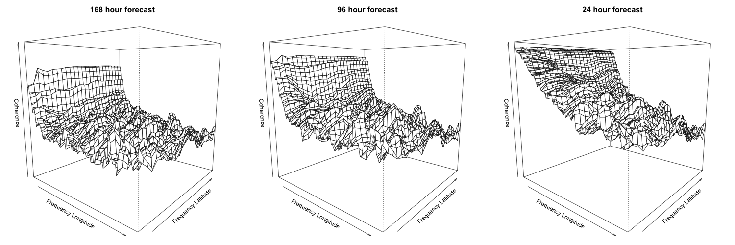
Figure 4: Estimated absolute coherence functions for the GEFS sea level pressure reforecast data, comparing the 168, 96 and 24 hour forecast horizons with the zero hour analysis. The vertical axis spans $[0,1]$.

Figure 4 shows estimated absolute coherence functions for horizons 168, 92 and 24h with the 0h analysis. Even at long lead lead times there is substantial coherence, which increases by a substantial margin at very low longitudinal frequencies. For any given longitude frequency band, the coherence appears to be relatively constant across latitudes, which is sensible given that there appears to be greater variability in the equatorial direction than in the north-south direction for sea level pressure in this region. As the forecast horizon decreases the coherence begins building between low-to-mid frequency bands in the latitudinal direction, suggesting that the statistical characteristics of short term forecasts are more similar to observed sea level pressure than the longer term forecasts. However, note that at the highest frequencies there is not a substantial improvement in forecast skill, bordering on no improvement, which suggests that small scale events are difficult to forecast even at one day out.

To quantify the differences in forecast horizon skill, we estimate a set of bivariate Matérn models. As each forecast and analysis arises from the same physical model, we assume that the marginal spectra follow the same statistical behavior, that is, we suppose the marginal spectral densities at equal at all horizons, $f_{00}(\boldsymbol{\omega})=f_{kk}(\boldsymbol{\omega})$. Suggested by Figure 4 and exploratory analysis for the marginal spectra, we additionally suppose the spectrum is constant across latitude frequencies. A Gaussianity assumption does not appear to be justifiable, based on empirical Q-Q plots. Thus, we follow the suggestion of Fuentes (2002) and estimate marginal Matérn parameters by minimizing the squared difference between theoretical log spectral density and log average periodogram, having averaged over all days, forecast horizons and latitude bands. The resulting least squares estimates are $a=0.074$ and $\nu=0.94$. Cross-covariance parameters are estimated by minimizing least squares distance to the average empirical coherence functions, estimated by averaging over days and latitude bands.

Table 1: Cross-covariance Matérn family parameter estimates for GEFS sea level pressure reforecast data.

Forecast horizon	24	48	72	96	120	144	168	192
$\rho$	0.96	0.94	0.91	0.88	0.85	0.81	0.76	0.73
$a_{12}$	0.079	0.076	0.075	0.073	0.071	0.070	0.068	0.067
$\nu_{12}$	1.06	1.06	1.05	1.04	1.03	1.02	1.01	1.01

Table 1 contains the cross-covariance parameter estimates corresponding to all forecast horizons. As forecast horizon increases, all parameters decay; in fact, the decay is almost exactly linear for each variable beyond the 24h horizon. Fitting a linear model to the parameters as a function of forecast horizon suggests the cross-covariance smoothness will decay to the marginal value $\nu=0.94$ after approximately 16 days, whereas the cross-covariance scale meets the marginal value between 3-4 days. Although these ideas can be used to generate scientific hypotheses, there is substantial extrapolation for $nu_{12}$ that strongly depends on a linear assumption.

A word of caution is in order; the estimates in Table 1 do not always imply a valid multivariate covariance structure. However, on any given grid the estimated parameters may yield a valid model, it just cannot be guaranteed for all grids. One possibility is that the bivariate Matérn is not sufficiently flexible to describe the stochastic structure of these fields, which is a call for further research in this area.

4.2 Geopotential Height

Our second example is on the same spatial domain, but whose values are geopotential heights. Geopotential height is the height (in meters) above sea level at which the atmospheric pressure is a certain level. In the atmospheric sciences, it is common to examine geopotential heights as indicators of climatic regimes, for instance Knapp and Yin (1996) examines the relationship between heights and temperature anomalies over a portion of the United States.

Three of the most common geopotential height maps are the 850hPa, 500hPa and 300hPa maps. The first, 850hPa, approximately defines the planetary boundary layer, which is the lowest level of the atmosphere that interacts with the surface of the Earth (note 1000hPa is approximately sea level). The 300hPa level is at the core of the jet stream, while the 500hPa approximately divides the atmosphere in half, and whose anomalies are used in part to assess climatological temperature variations. The vertical structure of geopotential heights is a focus of some interest within atmospheric sciences (Blackmon et al., 1979).

We examine geopotential height reanalysis anomalies $Z_{k}(\mathbf{s},d)$ for $k=1,2,3$ representing the 850hPa, 500hPa and 300hPa pressure levels on days $d=1,\ldots,181$, the first 6 months of 2014. The anomalies are differences between the reanalysis height and a time-varying Nadaraya-Watson kernel smoothed estimate of the mean with a bandwidth of 5 days. Experiments suggest the results below are qualitatively robust against choices of the bandwidth and smoothing kernel.

Similar to the previous section, we smooth the marginal process periodogram (13) using a low-pass filter, and calculate smoothed empirical cross-periodograms yielding $\{\tilde{I}_{ij}(\boldsymbol{\omega},d)\}_{i,j=1}^{3}$. Then the squared coherence is estimated as the arithmetic average of each day’s empirical squared coherence estimate,

$$\hat{\gamma}_{ij}(\boldsymbol{\omega})^{2}=\frac{1}{181}\sum_{d=1}^{181}\frac{|\tilde{I}_{ij}(\boldsymbol{\omega},d)|^{2}}{\tilde{I}_{ii}(\boldsymbol{\omega},d)\tilde{I}_{jj}(\boldsymbol{\omega},d)}.$$

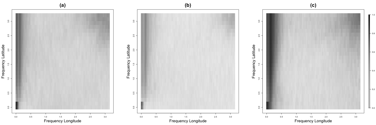
Figure 5: Estimated absolute coherence functions for the GEFS geopotential height data between (a) 850hPa and 500hPa, (b) 850hPa and 300hPa and (c) 500hPa and 300hPa.

Figure 5 contains the three estimated pairwise absolute coherence functions. There is high coherence between the lower pressure levels at low frequencies, and some evidence of moderate coherence between all levels at low frequencies. We also note some strikingly different behavior than for the sea level pressure example. First, there is an apparent ridge in coherence at low frequencies (approximately $2\pi 9/360$) which may be indicative of equatorial planetary waves (Wang and Xie, 1996; Xie and Wang, 1996; Kiladis et al., 2009). Planetary waves can play crucial roles in the formation of tropical cyclones (Molinari et al., 2007). Additionally, note that there is high coherence at the highest Fourier frequencies for all coherence functions (capping out at approximately $0.62,0.54,$ and $0.70$). This is evidence of a nonseparable relationship in the frequency domain, and we are unaware of any current multivariate models that can adequately capture such behavior. One possible explanation for this high coherence at high frequencies is artifacts in the data assimilation scheme, in particular aberrant observational data leading to unusually large anomalies in geopotential height. Indeed, variables such as sea level pressure are well constrained by a wealth of observational data, while geopotential heights are less constrained, usually being observed by sparsely released weather balloons.

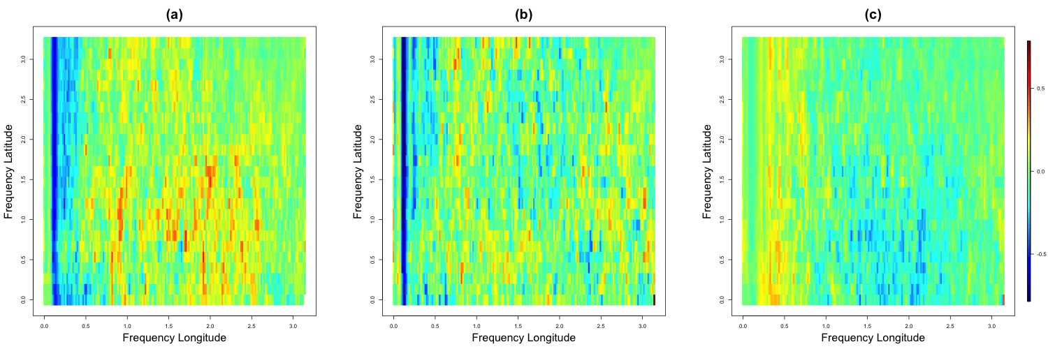
Figure 6: Estimated phase functions for the GEFS geopotential height data between (a) 850hPa and 500hPa, (b) 850hPa and 300hPa and (c) 500hPa and 300hPa.

Figure 6 shows pairwise plots for each pair of geopotential height anomalies. In particular there is strong evidence of a phase shift at a low frequency band between the 850hPa and both lower pressure heights. These frequencies indicate wavelengths of approximately $4000-6000$km, which is a typical wavelength for planetary equatorial waves, or Rossby waves (Wang and Xie, 1996; Xie and Wang, 1996; Kiladis et al., 2009). On the other hand, there is not substantial evidence of phase shift between the pairs of heights at other frequencies. Most extant multivariate models utilize real-valued cross-spectral densities, and thus are insufficiently flexible to capture this type of phase shifted behavior at specific spectra.

5 Discussion

The notion of coherence, phase and gain are common in the time series literature, but have been yet unexplored for multivariate spatial processes. We casted these functions for multidimensional processes. The coherence between two variables can be interpreted as a measure of linear relationship at particular frequency bands, resulting in a complementary framework for comparing processes than the usual cross-covariance function. Phase and gain also yield straightforward interpretations as a physical space-shift and relative amplitude of frequency dependence when comparing two processes. We developed these ideas for stationary processes, and future research may be directed toward the analogous cases for nonstationary processes, perhaps extending the work of Fuentes (2002).

Coherence, phase and gain can be estimated using smoothed cross-periodograms, and in our examples we showed that, as exploratory tools, these functions can be very useful in detecting structure that may not be readily captured using extant multivariate models. We additionally illustrated that the coherence function gives a natural interpretation to the multivariate Matérn cross-covariance parameters that have otherwise been uninterpretable, lending insight into an outstanding problem.

A number of future research directions may be considered, including the adaptation of coherence to multivariate space-time processes. This work can also be seen as a call to develop more flexible multivariate models, perhaps working directly in the spectral domain rather than the covariance domain, where most previous work has fallen, echoing the call of Simpson et al. (2015).

Appendix

The following Lemma is useful in proving some results of the manuscript.

Lemma 9.

Suppose $Z_{1}(\mathbf{s})$ is a stationary processes on $\mathbb{R}^{d}$ with covariance function $C_{1}(\mathbf{h})$ having spectral density $f_{1}(\boldsymbol{\omega})$ and $Z_{2}(\mathbf{s})=\int K(\mathbf{s}-\mathbf{u})Z_{1}(\mathbf{u}){\rm d}\mathbf{u}$ where $K$ is continuous, symmetric and square integrable with Fourier transform $f_{K}(\boldsymbol{\omega})$. Then $Z_{2}(\mathbf{s})$ has covariance function $C_{2}(\mathbf{h})=\int\int K(\mathbf{u}+\mathbf{v}-\mathbf{h})K(\mathbf{v})C_{1}(\mathbf{u}){\rm d}\mathbf{u}{\rm d}\mathbf{v}$ with associated spectral density $f_{2}(\boldsymbol{\omega})=f_{1}(\boldsymbol{\omega})f_{K}(\boldsymbol{\omega})^{2}$. Additionally, the cross-covariance function between $Z_{1}$ and $Z_{2}$ is $C_{12}(\mathbf{h})=\int K(\mathbf{u}-\mathbf{h})C_{1}(\mathbf{u}){\rm d}\mathbf{u}$ with spectral density $f_{12}(\boldsymbol{\omega})=f_{1}(\boldsymbol{\omega})f_{K}(\boldsymbol{\omega})$.

The proof of this Lemma involves straightforward calculations involving convolutions and is not included here.

We recall the spectral representation for a stationary vector-valued process $\mathbf{Z}(\mathbf{s})\in\mathbb{R}^{p},\mathbf{s}\in\mathbb{R}^{d}$ with matrix-valued covariance function $\mathbf{C}(\mathbf{h})$ having spectral measures $F_{ij},i,j=1,\ldots,p$ defined on the Borel $\sigma$-algebra ${\cal B}$ on $\mathbb{R}^{d}$. There is a set of complex random measures $\mathbf{M}=(M_{1},\ldots,M_{p})$ on ${\cal B}$ such that if $B,B_{1},B_{2}\in{\cal B}$ are disjoint, $\mathbb{E}M_{i}(B)=0,\mathbb{E}(M_{i}(B)\overline{M_{j}(B)})=F_{ij}(B)$ and $\mathbb{E}(M_{i}(B_{1})\overline{M_{j}(B_{2})})=0$ for $i,j=1,\ldots,p$. Then $\mathbf{Z}(\mathbf{s})$ has the spectral representation

$$\mathbf{Z}(\mathbf{s})=\int\exp(i\boldsymbol{\omega}^{\rm T}\mathbf{s}){\rm d}\mathbf{M}(\boldsymbol{\omega}),$$

see Gihman and Skorohod (1974) for details. If all $F_{ij}$ admit associated spectral densities $f_{ij}$, then in shorthand we write $\mathbb{E}({\rm d}M_{i}(\boldsymbol{\omega})\overline{{\rm d}M_{j}(\boldsymbol{\omega})})=f_{ij}(\boldsymbol{\omega}){\rm d}\boldsymbol{\omega}$.

Proof of Theorem 2.

The spectral representation implies

$$Z_{i}(\mathbf{s})=\int\exp(i\boldsymbol{\omega}^{\rm T}\mathbf{s}){\rm d}M_{i}(\boldsymbol{\omega}),$$

for complex-valued random measures $M_{i}$, $i=1,2$. Then if $K$ has Fourier transform $F_{K}$,

$$\int K(\mathbf{u}-\mathbf{s})Z_{2}(\mathbf{u}){\rm d}\mathbf{u} =\int\int K(\mathbf{u}-\mathbf{s})\exp(i\boldsymbol{\omega}^{\rm T}\mathbf{u}){\rm d}M_{2}(\boldsymbol{\omega}){\rm d}\mathbf{u}$$

$$=\int\exp(i\boldsymbol{\omega}^{\rm T}\mathbf{s})F_{K}(\boldsymbol{\omega}){\rm d}M_{2}(\boldsymbol{\omega})$$

by a change of variables. Then, using that $f_{ii}(\boldsymbol{\omega}){\rm d}\boldsymbol{\omega}=\mathbb{E}|{\rm d}M_{i}(\boldsymbol{\omega})|^{2}$ and

$$\mathbb{E}\left(\int g(\boldsymbol{\omega}){\rm d}M_{i}(\boldsymbol{\omega})\overline{\int h(\boldsymbol{\omega}){\rm d}M_{j}(\boldsymbol{\omega})}\right)=\int g(\boldsymbol{\omega})\overline{h(\boldsymbol{\omega})}f_{ij}(\boldsymbol{\omega}){\rm d}\boldsymbol{\omega}$$

we have

$$\mathbb{E}\left|Z_{1}(\mathbf{s})-\int K(\mathbf{u}-\mathbf{s})Z_{2}(\mathbf{u}){\rm d}\mathbf{u}\right|^{2} =\int\bigg{(}f_{11}(\boldsymbol{\omega})-f_{12}(\boldsymbol{\omega})F_{K}(\boldsymbol{\omega})-f_{21}(\boldsymbol{\omega})\overline{F_{K}(\boldsymbol{\omega})}+$$

$$\qquad F_{K}(\boldsymbol{\omega})\overline{F_{K}(\boldsymbol{\omega})}f_{22}(\boldsymbol{\omega})\bigg{)}{\rm d}\boldsymbol{\omega}$$

$$=\int\mathbb{E}\left|{\rm d}M_{1}(\boldsymbol{\omega})-F_{K}(\boldsymbol{\omega}){\rm d}M_{2}(\boldsymbol{\omega})\right|^{2}.$$

The integrand is minimized for each $\boldsymbol{\omega}$ if

$$F_{K}(\boldsymbol{\omega})=\frac{\mathbb{E}({\rm d}M_{1}(\boldsymbol{\omega})\overline{{\rm d}M_{2}(\boldsymbol{\omega})})}{\mathbb{E}|{\rm d}M_{2}(\boldsymbol{\omega})|^{2}}=\frac{f_{12}(\boldsymbol{\omega})}{f_{22}(\boldsymbol{\omega})}.$$

That the density of $\int K(\mathbf{u}-\mathbf{s})Z_{2}(\mathbf{u}){\rm d}\mathbf{u}$ is $|f_{12}(\boldsymbol{\omega})|^{2}/f_{22}(\boldsymbol{\omega})$ now follows by the convolution theorem for Fourier transforms. ∎

Proof of Proposition 4.

If $f_{i}(\boldsymbol{\omega})$ is the Fourier transform of $c_{i},i=1,2$, the result immediately follows as the spectral density of $C_{ij}(\mathbf{h})$ is $f_{i}(\boldsymbol{\omega})f_{j}(\boldsymbol{\omega})$. ∎

Proof of Proposition 5.

This result follows directly from Lemma 9. ∎

Proof of Proposition 6.

This result follows from Lemma 9 and that the spectral density for white noise is constant over all frequencies. ∎

References

- Apanasovich et al. (2012) Apanasovich, T. V., Genton, M. G., and Sun, Y. (2012), “A valid Matérn class of cross-covariance functions for multivariate random fields with any number of components,” Journal of the American Statistical Association, 107, 180–193.
- Berrocal et al. (2010) Berrocal, V. J., Gelfand, A. E., and Holland, D. M. (2010), “A bivariate space-time downscaler under space and time misalignment,” Annals of Applied Statistics, 4, 1942–1975.
- Bevilacqua et al. (2015) Bevilacqua, M., Hering, A. S., and Porcu, E. (2015), “On the flexibility of multivariate covariance models,” Statistical Science, in press.
- Bhat et al. (2010) Bhat, K. S., Haran, M., and Goes, M. (2010), “Computer model calibration with multivariate spatial output: a case study in climate parameter learning,” in Frontiers of Statistical Decision Making and Bayesian Analysis, eds. M. H. Chen, P. Müller, D. Sun, K. Ye, and D. K. Dey, pp. 401–408, Springer-Verlag, New York.
- Blackmon et al. (1979) Blackmon, M. L., Madden, R. A., Wallace, J. M., and Gutzler, D. S. (1979), “Geographical variations in the vertical structure of geopotential height fluctuations,” Journal of the Atmospheric Sciences, 36, 2450–2466.
- Brockwell and Davis (2009) Brockwell, P. J. and Davis, R. A. (2009), Time series: theory and methods, Springer Science & Business Media.
- Cramér (1940) Cramér, H. (1940), “On the theory of stationary random processes,” Annals of Mathematics, 41, 215–230.
- Cressie and Johannesson (2008) Cressie, N. and Johannesson, G. (2008), “Fixed rank kriging for very large spatial data sets,” Journal of the Royal Statistical Society, Series B, 70, 209–226.
- Fuentes (2002) Fuentes, M. (2002), “Spectral methods for nonstationary spatial processes,” Biometrika, 89, 197–210.
- Fuentes (2006) Fuentes, M. (2006), “Testing for separability of spatial-temporal covariance functions,” Journal of Statistical Planning and Inference, 136, 447–466.
- Gaspari and Cohn (1999) Gaspari, G. and Cohn, S. E. (1999), “Construction of correlation functions in two and three dimensions,” Quarterly Journal of the Royal Meteorological Society, 125, 723–757.
- Gaspari et al. (2006) Gaspari, G., Cohn, S. E., Guo, J., and Pawson, S. (2006), “Construction and application of covariance functions with variable length fields,” Quarterly Journal of the Royal Meteorological Society, 132, 1815–1838.
- Genton and Kleiber (2015) Genton, M. G. and Kleiber, W. (2015), “Cross-covariance functions for multivariate geostatistics,” Statistical Science, in press.
- Gihman and Skorohod (1974) Gihman, I. I. and Skorohod, A. V. (1974), The Theory of Stochastic Processes, Vol. 1, Springer-Verlag, Berlin.
- Gneiting et al. (2010) Gneiting, T., Kleiber, W., and Schlather, M. (2010), “Matérn cross-covariance functions for multivariate random fields,” Journal of the American Statistical Association, 105, 1167–1177.
- Goff and Jordan (1988) Goff, J. A. and Jordan, T. H. (1988), “Stochastic modeling of seafloor morphology: Inversion of sea beam data for second-order statistics,” Journal of Geophysical Research, 93, 13589–13608.
- Goulard and Voltz (1992) Goulard, M. and Voltz, M. (1992), “Linear coregionalization model: Tools for estimation and choice of cross-variogram matrix,” Mathematical Geology, 24, 269–282.
- Hamill et al. (2011) Hamill, T. M., Whitaker, J. S., Kleist, D. T., Fiorino, M., and Benjamin, S. G. (2011), “Predictions of 2010’s tropical cyclones using the GFS and ensemble-based data assimilation methods,” Monthly Weather Review, 139, 3243–3247.
- Hamill et al. (2013) Hamill, T. M., Bates, G. T., Whitaker, J. S., Murray, D. R., Fiorino, M., Galarneau Jr., T. J., Zhu, Y., and Lapenta, W. (2013), “NOAA’s second-generation global medium-range ensemble reforecast dataset,” Bulletin of the American Meteorological Society, 94, 1553–1565.
- Handcock and Stein (1993) Handcock, M. S. and Stein, M. L. (1993), “A Bayesian analysis of kriging,” Technometrics, 35, 403–410.
- Helterbrand and Cressie (1994) Helterbrand, J. D. and Cressie, N. (1994), “Universal co-kriging under intrinsic coregionalization,” Mathematical Geology, 26, 205–226.
- Hering et al. (2015) Hering, A. S., Kazor, K., and Kleiber, W. (2015), “A Markov-switching vector autoregressive stochastic wind generator for multiple spatial and temporal scales,” Resources, 4, 70–92.
- Kiladis et al. (2009) Kiladis, G. N., Wheeler, M. C., Haertel, P. T., Straub, K. H., and Roundy, P. E. (2009), “Convectively coupled equatorial waves,” Reviews of Geophysics, 47.
- Kleiber and Nychka (2015) Kleiber, W. and Nychka, D. W. (2015), “Equivalent kriging,” Spatial Statistics, 12, 31–49.
- Knapp and Yin (1996) Knapp, P. A. and Yin, Z. (1996), “Relationships between geopotential heights and temperature in the south-eastern US during wintertime warming and cooling periods,” International Journal of Climatology, 16, 195–211.
- Li and Zhang (2011) Li, B. and Zhang, H. (2011), “An approach to modeling asymmetric multivariate spatial covariance structures,” Journal of Multivariate Analysis, 102, 1445–1453.
- Lim and Stein (2008) Lim, C. Y. and Stein, M. (2008), “Properties of spatial cross-periodograms using fixed-domain asymptotics,” Journal of Multivariate Analysis, 99, 1962–1984.
- Majumdar and Gelfand (2007) Majumdar, A. and Gelfand, A. E. (2007), “Multivariate spatial modeling for geostatistical data using convolved covariance functions,” Mathematical Geology, 39, 225–245.
- Mardia and Goodall (1993) Mardia, K. and Goodall, C. (1993), “Spatial-temporal analysis of multivariate environmental monitoring data,” in Multivariate Environmental Statistics, eds. G. P. Patil and C. R. Rao, pp. 347–386, Amsterdam: North Holland.
- Molinari et al. (2007) Molinari, J., Lombardo, K., and Vollaro, D. (2007), “Tropical cyclogenesis within an equatorial Rossby wave packet,” Journal of the Atmospheric Sciences, 64, 1301–1317.
- Oliver (2003) Oliver, D. S. (2003), “Gaussian cosimulation: Modelling of the cross-covariance,” Mathematical Geology, 35, 681–698.
- Royle and Berliner (1999) Royle, A. and Berliner, L. M. (1999), “A hierarchical approach to multivariate spatial modeling and prediction,” Journal of Agricultural, Biological and Environmental Statistics, 4, 1–28.
- Schmidt and Gelfand (2003) Schmidt, A. M. and Gelfand, A. E. (2003), “A Bayesian coregionalization approach for multivariate pollutant data,” Journal of Geophysical Research – Atmospheres, 108.
- Simpson et al. (2015) Simpson, D., Lindgren, F., and Rue, H. (2015), “Beyond the valley of the covariance function,” Statistical Science, in press.
- Stein (1995) Stein, M. L. (1995), “Fixed-domain asymptotics for spatial periodograms,” Journal of the American Statistical Association, 90, 1277–1288.
- Stein (1999) Stein, M. L. (1999), Interpolation of Spatial Data: Some Theory for Kriging, New York: Springer-Verlag.
- Ver Hoef and Barry (1998) Ver Hoef, J. M. and Barry, R. P. (1998), “Constructing and fitting models for cokriging and multivariable spatial prediction,” Journal of Statistical Planning and Inference, 69, 275–294.
- Ver Hoef et al. (2004) Ver Hoef, J. M., Cressie, N., and Barry, R. P. (2004), “Flexible spatial models for kriging and cokriging using moving averages and the Fast Fourier Transform (FFT),” Journal of Computational and Graphical Statistics, 13, 265–282.
- Wackernagel (2003) Wackernagel, H. (2003), Multivariate Geostatistics, Berlin: Springer-Verlag, third edn.
- Wang and Xie (1996) Wang, B. and Xie, X. (1996), “Low-frequency equatorial waves in vertically sheared zonal flow. Part I: stable waves,” Journal of the Atmospheric Sciences, 53, 449–467.
- Xie and Wang (1996) Xie, X. and Wang, B. (1996), “Low-frequency equatorial waves in vertically sheared zonal flow. Part II: unstable waves,” Journal of the Atmospheric Sciences, 53, 3589–3605.
- Zhang and Zimmerman (2005) Zhang, H. and Zimmerman, D. L. (2005), “Towards reconciling two asymptotic frameworks in spatial statistics,” Biometrika, 92, 921–936.