Sharper asset ranking from total drawdown durations

Abstract

The total duration of drawdowns is shown to provide a moment-free, unbiased, efficient and robust estimator of Sharpe ratios both for Gaussian and heavy-tailed price returns. We then use this quantity to infer an analytic expression of the bias of moment-based Sharpe ratio estimators as a function of the return distribution tail exponent. The heterogeneity of tail exponents at any given time among assets implies that our new method yields significantly different asset rankings than those of moment-based methods, especially in periods large volatility. This is fully confirmed by using 20 years of historical data on 3449 liquid US equities.

1 Introduction

Sharpe ratios (Sharpe, 1964) appear naturally in financial analysis for a good reason: they are nothing else than signal-to-noise ratios, a fundamental quantity in signal analysis. In a Gaussian world, they are also equivalent to the t-statistics. Finance is not an ideal world, however, and many problems arise in practice. Sharpe ratio’s distribution (Lo, 2002), bias (Miller and Gehr, 1978; Jobson and Korkie, 1981) and corrections due to serial correlations (Lo, 2002; Mertens, 2002; Christie, 2005; Opdyke, 2007) have been characterized. Better estimating methods use the Generalized Moments Method (Lo, 2002; Christie, 2005) and block bootstraps (Ledoit and Wolf, 2008). Although Sharpe ratios only depend on the first and second moments of price returns, their variance depends on the third and fourth moments (Lo, 2002; Mertens, 2002; Christie, 2005; Opdyke, 2007). Given the definition of the Sharpe ratios, it is not surprising that all these methods rely on the computation of moments of price returns. But as noted e.g. in Opdyke (2007), this may be problematic as the fourth moment may not be defined (Dacorogna et al., 2001; Jondeau and Rockinger, 2003). Finally, the standard estimator of the Sharpe ratio is known be biased for heavy-tailed price returns. Once again, the corrections proposed e.g. for the Deflated Sharpe Ratio, depend on the third and fourth moment (Bailey and Lopez de Prado, 2014).

Here, I propose a new way to estimate Sharpe ratios that does not require the computation of any moment and that may be extended to estimate the drift of time series with infinite variance. It is based on the fact that the total duration of all drawdowns in a price time series of a given length is a monotonic function of the Sharpe ratio; by symmetry, the same holds for the total duration of all drawups. As a consequence, one may estimate Sharpe ratios by computing the difference between the total durations of drawups and drawdowns. This quantity is bounded by definition and leads to an estimator that is both robust to outliers and more efficient than direct estimates of Sharpe ratios for heavy-tailed data.

Above all, the new estimator is unbiased for heavy-tailed data, in contrast to the standard estimation method. Even more, we propose that the Sharpe ratio depends in a simple way of total drawdown durations and return distribution tail exponent, which allows a direct estimation of the bias of the moment-based estimator at fixed total drawdown duration length. This gives a new take on asset ranking: because all the asset price return distributions have different tail exponents at any point in time, the new method yields considerably different asset rankings, especially at the top and bottom quantiles, and during the most volatile periods. Thus this paper contributes both theoretically and empirically to the on-going debate about the relevance of the ranking method (Eling and Schuhmacher, 2007; Zakamulin, 2010; Schuhmacher and Eling, 2011; Ornelas, Silva Júnior, and Fernandes, 2012; Auer and Schuhmacher, 2013a, b)

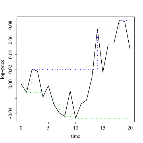
Figure 1: Example log price time series (black lines), its running maximum (blue dashed lines), and running minimum (green dashed lines). The number of upper (lower) records $R_{+}$ ($R_{-}$) is equal to the number of jumps of the running maximum (minimum) plus one since the first point counts as a record by convention: here $R_{+}=4$ and $R_{-}=7$. The total drawdown duration is $T_{-}=16$ and the total drawup duration is $T_{+}=13$. Clearly, $R_{+}+T_{-}=R_{-}+T_{+}=20+1$, the number of returns plus one.

Intuitively, the sum of all drawdown durations, i.e., the total drawdown duration of a time series of fixed length, is linked to the number of upper price records since a new price return pushes the price either to an all time high (a new upper record) or to a drawdown (see Fig. 1). This implies that if $n$ is the length of a price time series and $R_{+}$ is the number of its upper records ($R_{+}\geq 1$ because the first point is a record by convention), the total drawdown duration, denoted by $T_{-}$, is $T_{-}=n-(R_{+}-1)$. Because of this equivalence, total drawdown/up duration and the numbers of price records lead to two equivalent estimators; accordingly, we will use either wordings. Assuming that log prices are simple random walks, drawdown/up durations are determined by first-passage times, themselves derived from persistence (or survival) properties (Redner, 2001). The connection between persistence and price dynamics, especially in the context of market microstructure, is well known (Lo, MacKinlay, and Zhang, 2002; Eisler et al., 2009).

Persistence is at the core of a noteworthy recent result about discrete-time unbiased random walks. In a financial context, it may be stated as follows: the distribution of the number of upper (or lower) records of a price time series with independent and identically distributed return (i.i.d.), of a fixed length, does not depend on the increment distribution provided that the latter is symmetric and continuous (Majumdar and Ziff, 2008). This universality is behind the robustness and power of the r-statistics, a family of statistics based on the number of records of a time series, which not only provides a powerful non-parametric location test (Challet, 2015) but also, as shown here, an efficient estimator of Sharpe ratios. Their robustness come from the fact that the influence of outliers is much dampened because sample values are transformed into an integer number with bounded admissible values.

Majumdar, Schehr, and Wergen (2012) show that the distribution of the number of records converges to a Gaussian distribution in the limit of infinitely long time series provided that the price return distribution has a finite variance. Even better, the support of the finite-size sample distribution of the new estimator is bounded, contrarily to that of Sharpe ratios (and t-statistics), and is accordingly more peaked than a normal distribution (Challet, 2015). When the true Sharpe ratio is different from zero, the expected number of records and its variance are distribution-dependent; exact expressions are only known for exponentially distributed increments, hence one has to resort to approximations and numerical simulations for other types of distribution in the limits of large and small Sharpe ratios.

Drawdown durations are by definition integer numbers, which is not optimal to estimate a real number. The solution comes from random permutations. Assuming that the price returns are i.i.d., one can shuffle their order at will and compute the resulting price time series, which is an equally valid representation of a given set of price returns and most likely have a different number of upper and lower records. Thus, to obtain a more precise estimate of the Sharpe ratio, one takes the average of the difference between the total drawdown and drawup durations over many such permutations (see Fig. 3 for a graphical explanation).

The structure of this paper is as follows: Section 2 introduces the necessary notations to define price record statistics and shows that when prices have a positive trend, heavy-tailed increments lead to a larger number of upper price records than Gaussian increments; a mathematical derivation of the expected number of price records for Student’s t-distributed increments is reported in Appendix A, which focuses on the case of tail exponent equal to 4 (3 degrees of freedom) for the sake of analytical tractability. Section 3 investigates the efficiency of the number of price records as Sharpe ratio estimators relative to the vanilla estimator and shows that the new estimator is several times more efficient than moment-based methods for heavy-tailed variables and almost as efficient as the vanilla estimator in the case of Gaussian variables; it then derives a simple equation that simplifies the calibration of the relationship between true Sharpe ratio and estimated tail exponents and number of records. Section 4 uses an unbiased historical data set of 3449 liquid US equities to estimate 100-day rolling Sharpe ratios with both methods. It turns out that in leptokurtic times, the estimates from both methods may differ very significantly because the vanilla Sharpe ratio estimator is not only more volatile, but also systematically overestimates the information content of price time series that have heavy-tailed returns.

2 Record statistics of random prices

Financial data exist in discrete time, which will be the point of view adopted in this paper. Let us assume that the initial log price is $S_{0}=0$ and that its value at time $k>0$ follows

$$S_{k}=S_{k-1}+r_{k}+c$$ (1)

where $r_{k}$ is the increment at time $k$, assumed to be identically and independently drawn from a continuous distribution $P(r)$, and $c$ is a constant trend. Let the running maximum $M_{k}=\max_{1\leq t\leq k}S_{t}$ (see Fig. 1). The number of upper records of a time series of length $n$ is the number of jumps of $M_{n}$, which by convention always includes $M_{1}$; it will be denoted by $R_{+}$ and its distribution by $P(R_{+},n)$. In the same spirit, one defines $R_{-}$, the number of lower records, as the number of jumps of the running minimum.

Majumdar and Ziff (2008); Le Doussal and Wiese (2009); Majumdar, Schehr, and Wergen (2012) demonstrate that many quantities of interest are fully characterized by the persistence function $q_{-}(n)$ of the process, i.e., the probability that the price has never exceeded its starting value after $n$ steps. It is advantageous to work with its characteristic function $\tilde{q}_{-}(z)=\sum_{n>0}z^{n}q_{-}(n)$.

For example, the characteristic function of $P(R_{+},n)$ is (Majumdar and Ziff, 2008)

$$\tilde{P}(R_{+},z)=\tilde{q}_{-}(z)[1-(1-z)\tilde{q}_{-}(z)]^{R_{+}-1},$$

while the characteristic function of the expected number of upper records $m_{+}(n)=E(R_{+})(n)$ can be written as $\tilde{m}_{+}(z)=[(1-z)^{2}\tilde{q}_{-}(z)]^{-1}$ (Le Doussal and Wiese, 2009).

Generalized Sparre Andersen theorem (Andersen, 1953; Feller, 2008) provides a constructive way to compute $\tilde{q}_{-}$: for any continuous and symmetric $P(r)$,

$$\log\left(\tilde{q}_{-}(z)\right)=\sum\limits_{n=1}^{\infty}\frac{z^{n}}{n}P(S_{n}<0).$$ (2)

2.1 Driftless prices

A direct consequence of this theorem is the universality of the unbiased case $c=0$ since $P(S_{k}<0)=\frac{1}{2}$ for all symmetric and continuous distributions, as indeed $\tilde{q}_{\pm}(z)=\tilde{q}(z)$ is the same for all such distributions and

$$P(R,n)={2n-R+1\choose R}2^{-2n+R-1},$$

where $R$ may either be $R_{+}$ or $R_{-}$, by symmetry (Majumdar and Ziff, 2008). This implies that the first two moments of this distribution are

$$E(R_{\pm})(n)\simeq 2\sqrt{\frac{n}{\pi}},~{}~{}~{}\textrm{and}~{}~{}~{}~{}E[((R_{\pm}-E(R_{\pm}))^{2}](n)\simeq(2-4/\pi)n.$$

2.2 Limit of small relative drift

Analytical results are harder to obtain in the case of non-zero drift ($c\neq 0$) since Sparre Andersen theorem requires the full knowledge of all convolutions of the elementary increments. Denoting the standard deviation of the increments $r_{k}$ by $\sigma$, good approximations of the expected number of upper records are known for Gaussian increments in the limit of small relative drift, i.e., when $c/\sigma\ll 1$ and $n\gg 1$ while $cn/\sigma\ll 1$ (Wergen, Bogner, and Krug, 2011; Majumdar, Schehr, and Wergen, 2012):

$$E(R_{+})(c/\sigma,n)\simeq 2\sqrt{\frac{n}{\pi}}+\frac{c\sqrt{2}}{\sigma\pi}\left[n\arctan(\sqrt{n})-\sqrt{n}\right].$$ (3)

The case of heavy-tailed increments with finite variance has not been thoroughly investigated. We will focus on Student’s t-distributions because of their abilities to reproduce both fat-tailed and Gaussian returns. They are known to describe the unconditional price return distribution (i.e., forgetting about volatility heteroskedasticity) (Bouchaud and Potters, 2000; Longin, 2005; Opdyke, 2007) and innovations (see e.g. Bollerslev (1987)). Let us therefore assume from now on that the price returns $r_{k}$ are distributed according to a Student’s t-distribution of variance $\sigma^{2}$ with $\nu$ degrees of freedom (we use this wording only to parametrize the return distribution), denoted by $P(r)$. Sparre Andersen theorem requires the knowledge of the $n$-time convoluted return distribution, denoted by $P^{(n)}(r)$, of which no explicit expression exists for generic values of $n$ and $\nu$. In passing, $P^{(n)}(r)$ can be explicitly computed for any value of $n$ provided that $\nu$ is odd but the expressions quickly become cumbersome as $n$ grows (Nadarajah and Dey, 2005). This is why we shall resort to approximations.

Appendix A reports approximate analytical results for the case $\nu=3$, i.e., for a tail exponent of 4. The resulting expected number of upper records becomes, in the same limit $c/\sigma\ll 1$ and $n\gg 1$ while $cn/\sigma\ll 1$,

$$E(R_{+})(n,c/\sigma) \simeq \frac{2\sqrt{n}}{\sqrt{\pi}}+\frac{c\sqrt{2}}{\sigma\pi}\left[n\arctan(\sqrt{n})-\sqrt{n}\right]$$ (4)

$$+\frac{c}{\sigma}\frac{8}{\sqrt{3}\pi^{3/2}}\sqrt{n}\left(\mbox{atanh}\sqrt{1-\frac{1}{n}}-\sqrt{1-\frac{1}{n}}\right).$$

Although a first order expansion, Eq. (4) is not very accurate even in the limit of small $n(c/\sigma)$, because the approximations needed to obtain explicit equations are quite rough (see Fig. 2). However, it was worth computing it for several reasons. First, it contains the correct dependence of $E(R_{+})(n,c/\sigma)$ on $n$ for small Sharpe ratios, which means that one may use this functional form to fit numerical simulations. Second, the presence of the third term, due to the difference between Gaussian and t-distributions at the origin, correctly implies that the prices with positive trends and heavy tails (and small Sharpe ratios) have a larger expected number of price records, which emphasises the importance of accounting for the tails of price return distributions when using price records to estimate Sharpe ratios (cf. section 3).

Appendix B contains the derivation of $E(R_{+})(n,c/\sigma)$ in the large relative drift limit, i.e., $c/\sigma\gg 1$ and $n\gg 1$. In this case, the expected number of records grows linearly.

It is noteworthy that these limits do not unequivocally correspond to small and large Sharpe ratios, since the limits do not involve $n^{1/2}$ but $n$. The small effective drift limit can be rewritten as $c/\sigma\sqrt{n}\ll 1/\sqrt{n}$, which correspond to vanishingly small Sharpe ratios, of little relevance to Finance; there is no guarantee that the very large $c/\sigma$ limit corresponds to realistic situations. Thus, depending on both $c/\sigma$ and $n$, one may be close to either limit, or in a no limit’s land. As a consequence, the next section resorts to extensive numerical calibration.

Figure 2: Excess number of records $E(R_{+}|c/\sigma,n)-E(R_{+}|0,n)$ for biased random walks with Student-t increments ($\nu=3$). Interrupted lines are theoretical predictions and continuous lines are from numerical simulations. $c=0.001$, $\sigma=1$, averages over $10^{7}$ samples.

3 Moment-free Sharpe ratio estimator

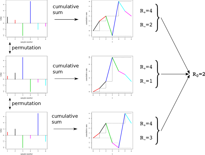
Figure 3: Schematic explanation of the idea behind the permutation estimator of Sharpe ratios: one computes the difference between total drawup and drawdown durations, or equivalently, the number of jumps of the running maximum (dashed lines) and the number of jumps of the running minimum (dotted lines) of the cumulated sums of the sample values, averaged over many random permutations of the price returns. By convention, the first point counts as a first record for both the running maximum and minimum.

As shown by Majumdar, Schehr, and Wergen (2012), the expected number of records is a monotonous function of the ratio $c/\sigma$, hence, of the Sharpe ratio. In other words, there is a one-to-one correspondence between the two quantities. This implies that it is possible to estimate Sharpe ratios from the number of upper or lower records. More precisely, we have

$$E(R_{+})=F_{+}(c/\sigma),$$ (5)

which implies that

$$\hat{\left(\frac{c}{\sigma}\right)}=F_{+}^{-1}(\hat{R}_{+}).$$ (6)

Because of the lack of exact results, we shall use numerical simulations to calibrate $F$.

The main problem of a number of records is that it is an integer number by definition, which yields an estimator with unacceptable precision for short time series. The fundamental idea of the r-statistics (Challet, 2015), in this context, consists in assuming that its log returns are i.i.d.. In that case, one may build many other log price paths based on random permutations of the original returns and thus measure the average number of records of the cumulated sums over many permutations (see Fig. 3) (this scheme may be extended to correlated time series). Mathematically, denoting the random permutation of index $i\in\{1,\cdots,n\}$ by $\pi(i)$ and the ensemble of all permutations by $\Pi$, the average number of records is $\bar{R}_{+}=\frac{1}{|\Pi|}\sum_{\pi\in\Pi}R_{+,\pi}$ where $R_{+,\pi}$ is the number of upper records of $S_{n,\pi}=\sum_{m=1}^{n}r_{\pi(m)}$. In practice, one restricts computations to a subset of $\Pi$ for the sake of computational tractability, which has little influence on the end result; in this study, we have used 1000 random permutations. The new Sharpe ratio estimator is then based on $R_{0}=\bar{R}_{+}-\bar{R}_{-}$. More precisely, the idea is to first calibrate the relationship $E(R_{0})=F_{0}(c/\sigma,n)$ at fixed $c/\sigma$ for a given distribution of synthetic price returns. Denoting $\theta=c/\sigma$, one then inverts this relationship to obtain

$$\hat{\theta}=F^{-1}(\hat{R}_{0},n).$$ (7)

Estimation in the rest of this paper is based on extensive numerical simulations to establish the relationships $E(R_{0})$ as a function of parameters $n$, $\theta$, and the Student parameter $\nu$. We chose $\nu=\{2.5,\cdots,10\}$ with increments of 0.1, $10<n<375$ by steps of 5 and $n=504$; we take 31 values of $\theta\in[0.001,1]$ growing according to a geometric series. For each triple $(n,\theta,\nu)$, we generate $N_{avg}$ synthetic time series, estimate $R_{0}$ over 1000 random permutations for each time series and then average $R_{0}$ over the $N_{avg}$ time series. Splines are then used to fit and invert the relationships of Eq. (7).

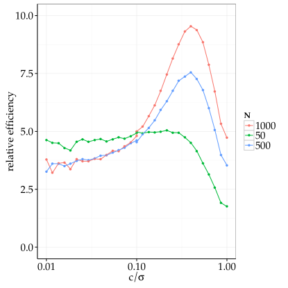
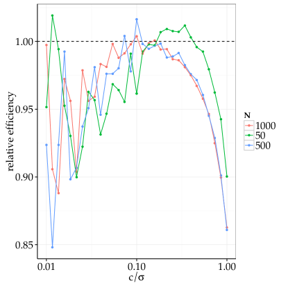
Figure 4: Efficiency of the record-based estimator $\theta_{0}$ relative to that of the vanilla estimator, defined by the ratio of the variance of the new estimator $\theta_{0}$ and the usual one $\theta_{S}$ as a function of the true Sharpe ratio $c/\sigma$ of the synthetic data. Averages over $N_{avg}=10^{6}$ samples per point; record numbers have been averaged over $1000$ permutations; left plot: Student-distributed increments with tail exponent set to 4; right plot: Gaussian increments.

3.1 Efficiency

Moment-based estimators have a hard time with heavy-tailed data. It is thus clear that their precision, i.e., efficiency, suffer from heavy tails. The new estimator, on the other hand, is likely to be less affected by the latter.

In order to compare their respective efficiency, let us denote by $\theta_{0}$ the Sharpe ratio inferred from $R_{0}.$ The standard deviation of $\theta_{0}$, denoted by $\sigma_{\theta}$, is obtained by the method of Deltas, i.e., from the relationship $\sigma_{\theta}=\sigma_{R}\frac{1}{\frac{dE(R_{0}|n,\theta)}{d\theta}}$ where $\sigma_{R}$ is the standard deviation of $R_{0}$; the numeric derivative of $E(R_{0}|n,\theta)$ was computed numerically with splines. The relative efficiency of $\theta_{0}$ with respect to the straightforward estimator $\theta_{S}=\hat{\mu}/\hat{\sigma}$ is then defined as $\rho=\sigma_{S}^{2}/\sigma_{R}^{2}$ where $\sigma_{S}$ is the standard deviation of $\theta_{S}$. Left plot of Fig. 4 reports the relative efficiency of $\theta_{0}$ for various $n$ for Student’s t-distributed returns and $\nu=4$. The new estimator is unambiguously more powerful than the vanilla estimator. This result holds as long as the returns are heavy tailed.

Financial price returns are not heavy tailed all the time. Thus it is important to check the efficiency of record statistics for log prices with Gaussian increments. Since the vanilla estimator is asymptotically optimal in this case (Neyman and Pearson, 1933), any other estimator is bound to be less efficient for large $n$. The right hand side plot of Fig. 4 plots the relative efficiency of $\theta_{0}$ for Gaussian increments, which depends on $c/\sigma$. Remarkably, $\theta_{0}$ may be slightly more efficient than the t-statistics itself for small $n$.

3.2 Dependence on Student tail exponent

Although only the $\nu=3$ was studied analytically above, as it leads to workable expressions, the relationship between $E(R_{0})$ and the Sharpe ratio of increments with a Student’s t-distribution depends on $\nu$. As a consequence, at fixed $n$ and $R_{0}$, the estimated Sharpe ratio also depends on $\nu$. Extensive numerical simulations (see Fig. 5) with $N_{avg}=10^{5}$ show that, at fixed $R_{0}$ and $n$,

$$E_{\nu}(\hat{\theta})=a(R_{0},n)-b(R_{0},n)\nu^{-3/2},$$ (8)

where $a(R_{0},n)=E_{\infty}(\hat{\theta})$ corresponds by definition to the average (and unbiased) Sharpe ratio of a process with Gaussian increments ($\nu\to\infty$).

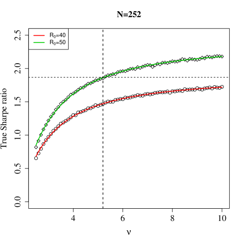
Figure 5: True Sharpe ratio versus Student tail index $\nu$ for $R_{0}=40$ and $50$ (circles and lozanges, respectively) for time series of length 252. The continuous lines are least-squares regressions to Eq. (8). The horizontal dashed line reports the value of the true Sharpe ratio for Gaussian increments ($\nu\to\infty$) and $R_{0}=40$, while the vertical one stands at $\nu=5.2$, which is the threshold at which the respective rank switches if a time series with $R_{0}=40$ and $\nu=\infty$ is compared with one with $R_{0}=50$ and with exponent $\nu$.

In addition to providing a simple way to extend the inference of the Sharpe ratio for arbitrary large values of $\nu$ from a finite interval of $\nu$, this equation quantifies the bias of an estimation of Sharpe ratios if one neglects the effect of non-Gaussian returns. Indeed, the estimation of $R_{0}$ does not require any assumption about the underlying increment distribution, only the connection to the Sharpe ratio does. This means that estimating Sharpe ratios requires estimating $\nu$, and that assuming $\nu=\infty$, as the vanilla method does, overestimates the true value of the Sharpe ratio as soon as the price return distribution has fatter tails than a Gaussian one. As a consequence, results about the equivalence of ranking from various methods only hold if all the assets have the same tail exponent. This point is further discussed in section 4.1.

3.3 Simplified estimation

Equation (8) provides a great complexity reduction in the estimation of the Sharpe ratio, but estimation may be further simplified by studying the dependence of both $a$ and $b$ on $R_{0}$ and $n$. We choose values of $R_{0}$ from 1 to $n$, and inferred the corresponding values of $\theta$ thanks to the calibrated relationships of Eq.  (7). Then, at fixed $n$, we choose a value $R_{0}$ and perform the non-linear fit of Eq. (8), which yields $a(R_{0},n)$ and $b(R_{0},n)$. We then filter out fits whose p-value associated with $b$ is larger than 0.01 and whose average square residual is larger than 0.1, which only happens in regions with large $n$ and small $R_{0}$ (in other words, where $\hat{\theta}=0$ is a fairly good approximation of the true Sharpe ratio). This leaves 13282 values of $a$ and $b$, one for each remaining couple $(R_{0},n$).

Let us start with $a=E_{\infty}(\hat{\theta})$. Left plot of Fig. 6 shows that $a(R_{0},n)=a(R_{0}/n)$ for $n>100$: the collapse, while not perfect, is remarkable (there are 12645 points in this figure). In other words, $R_{0}\simeq\gamma n$ with fixed $\gamma$ at least for $n>100$ and $\theta>0.001$ (a t-statistics of 0.01), as in the large $\theta n$ limit, although $n\theta=0.1$ in this case is far from being large. Figure 6 also makes it clear that $1-R_{0}/N$ decreases faster than an exponential, which makes sense since it asymptotically follows a Gaussian function (cf. Appendix B). Note that the scaling $R_{0}\propto n$ assumes that price returns do have a trend. In other words, the Sharpe ratio in the region where $R_{0}\propto\sqrt{n}$ will be under-estimated, but they correspond to negligible trends.

Let us now turn to $b(R_{0},n)$. It turns out that there is a linear relationship $b\simeq 8/3a$ in the region $a<1$ (see the right plot of Fig. 6), the collapse being remarkable. This region is relevant to Finance: for example, if $a=1$, and $n=100$, the t-statistics would be $10$, a rarity. Thus, the whole calibration may rest on the determination of $a(R_{0}/n)$, since

$$\hat{\theta}\simeq a(\hat{R}_{0}/n)\left[1-\frac{8}{3}\hat{\nu}^{-3/2}\right]$$ (9)

As $a$ is a smooth function, we first round $R_{0}/n$ to a precision of 0.01, and compute the average of $a(r)$ where $r$ is the rounded value of $R_{0}/n$. Finally, a spline is calibrated on this coarse-grained relationship, with the additional the coordinates (0,0) for the sake of convergence for very small values of $R_{0}/n$. Thus, simple scaling arguments made it possible to build an numerical estimation method for any $n$, $\nu$ and $R_{0}$ that rests on a single function.

  

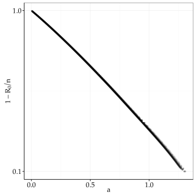
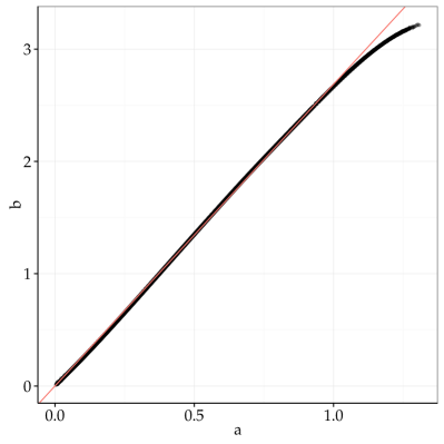
Figure 6: Left plot: collapse plot showing the scaling relationship between $a=E_{\infty}(\hat{\theta})$ and $R_{0}/n$ for 12465 couples $(R_{0},n)$, with $100<n<504$; the y axis is in log scale. Right plot: $b$ as a function of $a$, and a linear fit $b\simeq 2.67a$ for $a<1$; same parameters as in the left plot.

4 Application to real data

The i.i.d. assumption is totally unrealistic regarding asset price returns, if only because of volatility heteroskedasticity. Applying straightforwardly the above estimator would therefore make little sense on long time series. The approach followed here is to consider smaller time windows and to assume that stationarity approximately holds in each time window. The second current limitation of the proposed estimator to keep in mind here is that it does not account explicitly for skewness. At any rate, this section is meant to provide a clear illustration of how different the estimates of both methods may be.

In order to find the corresponding Sharpe ratio, we assume that price returns are conditionally leptokurtic (Bollerslev, 1987): in each time window, we fit the returns with Student’s t-distribution by maximum likelihood and obtain an estimate $\hat{\nu}$ and use Eq.  (9).

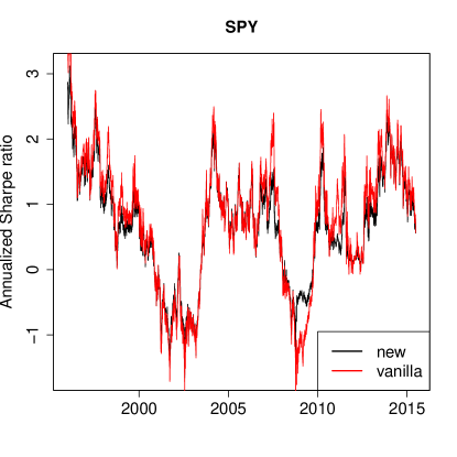
Figure 7: Left plot: parametric fit of the number of degrees of freedom of Student’s t-distribtuion in a sliding window of 252 close-to-close returns of SPY. Right plot: estimated Sharpe ratios with the new estimator and from a vanilla estimation. 1000 permutations have been used to estimate $R_{0}$.

Figure 7 shows the difference between annualized Sharpe ratios of SPY estimated with the new and vanilla estimator. When $\nu$ is larger that 10, both estimators yield almost the same Sharpe ratio, as expected from Eq. 8. On the other hand, when tails are heavier, i.e. when $\nu<10$, the two estimates significantly differ. Indeed, the new term in Eq. (4) with respect to Eq. (3) implies that vanilla estimates are too large in absolute values. This is confirmed in Fig. 8. The difference between both estimates is very large in leptokurtic times, e.g. in 2008 and 2009; in addition, in these difficult times, the new estimator is clearly less volatile, which is in line with its better efficiency.

Figure 8: Discrepancy of the estimates of the annualized Sharpe ratio of SPY with moving time windows of 252 days between the new and the vanilla estimators. 1000 permutations have been used to estimate $R_{0}$.

As a side note, the fact that the moment-based method overestimates the Sharpe ratio (and the t-statistic) in leptokurtic times means that using it for trading purposes leads to taking wrong trading decisions more often (the power of the r-statistics is indeed much larger than that of t-statistics for heavy-tailed data (Challet, 2015)). Let us try the following naive trading strategy (without transaction costs): whenever the estimated annualized Sharpe ratio is larger than 1 in absolute value in the last 100 close-to-close price returns, one takes a long or short single-day position, depending on the sign of the Sharpe ratio (with a one day lag). We use an unbiased historical data set of US equities (1995-01-01 to 2015-06-30) and focus on liquid assets, i.e. whose price is larger than $20 and 60-day rolling median daily volume is larger than 250000 shares. Figure 9 reports the cumulated performance of this strategy when applied to all 3449 US equities for the period . The difference of performance between the two methods is marked in times of large fluctuations (e.g. 2008). Note that the y-axis of this plot is logarithmic so as to avoid fooling the reader (McLean, 2011); in addition, it should be noted that the out-of-sample performances plotted in Fig. 9 is the result of 3449 decisions at each time step, i.e., very many decisions. As a consequence, the origin of the difference of performance between the new and vanilla methods is the relative power of the related statistical tests (Challet, 2015), not an erroneous way of computing compounded returns.

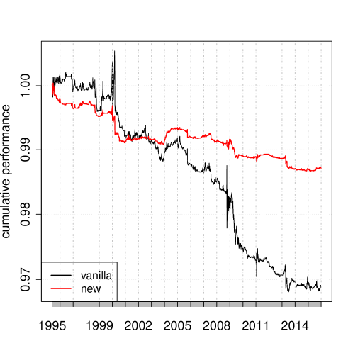
Figure 9: Cumulated performance of a trading strategy consisting in investing when the estimated annualized Sharpe ratio is larger than 1 in absolute value; short positions are allowed in case of negative Sharpe ratio; estimates over rolling windows of 100 trading days (close-to-close price returns). Unbiased historical database of 3449 US liquid equities. 1000 permutations have been used to estimate $R_{0}$.

4.1 Ranking assets

It is worth discussing the relevance and practical value of the proposed Sharpe ratio estimator beyond its much improved precision in leptokurtic times and the appreciable fact that it is unbiased. The industry is not only interested in the actual Sharpe ratio values of a group of assets (stocks, hedge funds, etc.), but also in ranking them. Thus, an important question is to assess whether the new method ranks assets in a different way than vanilla Sharpe ratio estimation. If this is clearly not the case, by extension, the new method brings a valuable alternative way to rank assets.

Two preliminary remarks. First, the fact that both methods estimate the same quantity, but that one method is clearly much more efficient for non-Gaussian variables implies that the correlation of the asset ranks cannot be 1 because of the greater fluctuations of the vanilla estimator. Second, as explained above, the Sharpe ratio corresponding to an estimated $R_{0}$ depends on the tail index of the Student distribution. Since the new method is unbiased and the vanilla one is biased for heavy-tailed distribution, and since the estimated tail exponents at any given time will vary from asset to asset, one cannot expect the two methods to yield on average equivalent ranking, even asymptotically. In other words, the location-shape argument of Schuhmacher and Eling (2011) does not hold for assets with heterogeneous tail indices, as noted e.g. in Zakamulin (2010).

Let me take an example: looking once again at Fig. 5 makes it clear that the ranking of $R_{0}$, i.e., of the vanilla estimation method, may not be the same one as the ranking according to the new method. Assume that asset 1 has $R_{0,1}=40$ and asset 2 $R_{0,2}=50$; neglecting the fact that $\nu_{1}<\infty$ and $\nu_{2}<\infty$ is quite possible, the vanilla method attributes a better rank to asset 2. Now, say $\nu_{1}=10$; as soon as $\nu_{2}<4.4$, asset 1 must be attributed a better rank than asset 2 (provided that the estimations of the tail exponents are precise enough).

All the above shows the crucial role of $\nu$ and sheds a new light on the debate on whether all risk measures are equivalent asymptotically or not. The point is that many of them may be biased for non-Gaussian variables in an equivalent way. For example, Auer and Schuhmacher (2013b) find that the rankings of hedge fund performance with the largest Sharpe ratios are most stable. But its results rest on measures that overestimate Sharpe ratios for heavy-tailed returns; thus, as sizeable fraction of these large Sharpe ratios may simply be the results of the methods’ biases.

Let me first focus on the 5% best and worst estimated Sharpe ratios. Figure 10 (left plot) shows that the fraction of common assets in these centiles is significantly different from 1, except notably for positive Sharpe ratios in 2008. As expected, this fraction decreases when the heterogeneity of tail exponents increases (right plot).

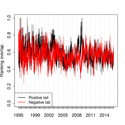
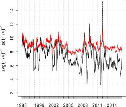
Figure 10: Left: evolution of the fraction of common assets between rankings for the moment-free and vanilla Sharpe ration estimation methods; black lines: top 5% positive ratios, red lines: smallest 5% ratios; calibration over 100 days; unbiased historical database of 3449 liquid US equities. Right: effective measure of average (red lines) and standard deviation (black lines) of tail exponents as a function of time for the 3449 US equities.

As expected, rankings differ more for assets with a small $\nu$, i.e., with heavy tails. Left plot of Fig. 11 reports the time evolution of Spearman and Kendall rank correlation of all the assets for both methods. As in Auer and Schuhmacher (2013b), an alternative rank correlation measure (Blest, 2000; Genest and Plante, 2003), more sensitive to the rank of the largest values of data, is displayed in the right hand side of this figure; it is slightly above zero on average, with large fluctuations in 2003 and 2009, which echoes the decrease of both Spearman and Kendall correlations at those dates, but not at other dates. Thus, ranking equities with usual moment-based methods or the new moment-free method may yield very significantly different results in the case of daily price return of equities. Hedge fund performance returns have a monthly resolution and are thus much closer to Gaussian variables, owing to the central limit theorem (see e.g. Bouchaud and Potters (2000)), which may also explain why previous studies did not find striking differences of ranking for most performance measures.

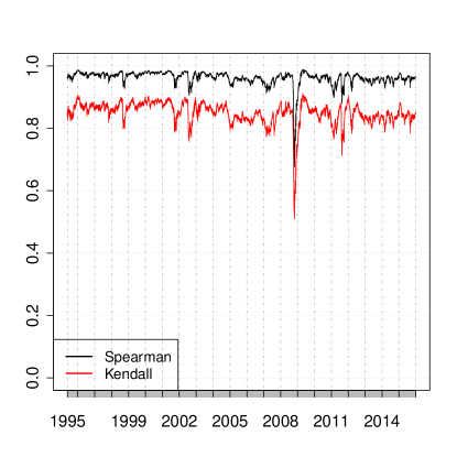
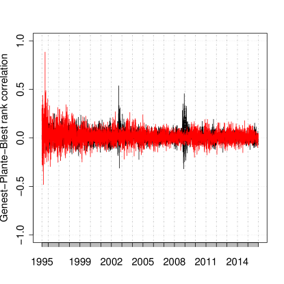
Figure 11: Spearman, Kendall (left plot) and Genest-Plante-Blast (right plot) rank correlations between the ranks of the Sharpe ratios obtained by record statistics and the usual method as a function of time (black lines: positive Sharpe ratios, red lines: negative Sharpe ratios). Sliding calibration windows of 100 days.

5 Discussion

The proposed Sharpe ratio estimator is robust, efficient, and well-behaved as it does not rely on moment estimation. Large returns are not regarded as outliers, but contribute to record statistics in a smooth way. In addition, a real outlier (due e.g. to a data error, or a neglected corporate action) may only create a single spurious additional price record, while two outliers of the same magnitude and opposite signs have only a mild influence on $R_{0}$. Finally, the robustness of the estimator lies in the fact that the latter is based only on the duration of drawdowns, not on their amplitudes. This is to be contrasted with other quantities related to drawdowns. For example the expectation of the maximum drawdown of a Brownian motion is a known function of the Sharpe ratio (Magdon-Ismail et al., 2003), but is very sensitive to outliers by definition.

Because of the lack of exact results, using this estimator requires for the time being numerical calibration, which has been much simplified by scaling arguments. Estimating Sharpe ratios with price record/drawdown statistics is not limited to Student’s t-distributed returns, as indeed one may calibrate their relationships for any return distribution with finite variance. In addition, the method introduced in this paper provides a generic way to build many types of estimators with record statistics as long as the relationship between price record statistics and the measurable to estimate is monotonic. For example, it may be used to estimate the drift of a Lévy process.

The main limitations of the proposed estimator are the assumptions of i.i.d and symmetric increments. Both can be accounted for numerically for the time being. An interesting challenge is to incorporate serial correlations into the analytical computation of record statistics: numerical results point to simple corrections in the case of AR(1) and GARCH(1,1) models (Wergen, 2014). Practically, a way to respect return auto-correlation and volatility heteroskedasticity is to use a kind of block-bootstraps, as in Ledoit and Wolf (2008).

An R package entitled sharpeRratio implements the new estimator and is available on CRAN at https://cran.r-project.org/web/packages/sharpeRratio/index.html; a Python version is available at PyPi https://pypi.python.org/pypi/pysharperratio/0.1.10.

An interactive webpage which reproduces the plots of Section 3 for any asset symbol and time period may be found at
https://brillant.shinyapps.io/moment-free_Sharpe_ratio .

Appendix A Expected number of records in the vanishing Sharpe ratio limit for Student’s t-distributed price returns

In this limit, one may use a first order expansion of the reciprocal cumulative function

$$P(S_{n}>0)=\frac{1}{2}+P^{(n)}(0)cn+O([cn]^{2}).$$ (10)

One therefore needs to compute $P^{(n)}(0)$. Since the increments are assumed to be independent,

$$P^{(n)}(0)=\frac{1}{2\pi}\int_{-\infty}^{\infty}\phi^{(n)}(t)dt=\frac{1}{2\pi}\int_{-\infty}^{\infty}[\phi(t)]^{n}dt,$$

where $\phi^{(n)}(t)$ is the characteristic function of $P^{(n)}(x)$, and $\phi(t)$ that of $P^{(1)}(r)=P(r)$. Equation (10) requires the computation of $P^{(n)}(0)$, which is impossible for any $n$ and $\nu$. However the $\nu=3$ case leads to workable expressions. One finds $P^{(n)}(0)=\frac{e^{n}}{\sigma\pi}E{}_{-n}(n)$, where $E_{n}(z)$ is the exponential integral function. The specific form $n=-z$ of the exponential integral function is easy to compute in a recursive way by integration by parts:

$$E_{-k-n}(k) = \frac{e^{-k}}{k}+\frac{k-n}{k}E_{-(k-n-1)}(k)$$

$$E_{0}(k) = \frac{e^{-k}}{k}.$$

Therefore, after some elementary computations, $E_{-n}(n)=\frac{e^{-n}}{n}\frac{n!}{n^{n}}\left(\sum_{s=0}^{n}\frac{n^{s}}{s!}\right)$ and

$$P^{(n)}(0)=\frac{1}{\sigma\pi}\,\frac{1}{n}\,\frac{n!}{n^{n}}\sum_{s=0}^{n}\frac{n^{s}}{s!}.$$ (11)

Using the asymptotic expansion $K_{n}=\sum_{s=0}^{n}\frac{n^{s}}{s!}=e^{n}[\frac{1}{2}+\sqrt{\frac{2}{3\pi}}\frac{1}{\sqrt{n}}+O(n^{-1})]$ and the usual Stirling expansion, Eq. (11) becomes $P^{(n)}(0)=\frac{1}{\sigma}\frac{1}{\sqrt{2\pi n}}+\frac{2}{\sigma\pi\sqrt{3}n}+O(n^{-3/2})$ and thus, in the case of small drifts, Eq. (10) reads

$$P(S_{n}>0)=\frac{1}{2}+\frac{c}{\sigma}\frac{2}{\pi\sqrt{3}}+\frac{c}{\sigma}\sqrt{\frac{n}{2\pi}}+O(n^{-1/2}).$$

Higher-order expansions of $K_{n}$ and $n!$ contribute terms of order $n^{-1/2}$ that are negligible. It is noteworthy that the additional correction for Student increments does not depend on $n$; accordingly, it is relevant for any value of $n$ and has a larger relative weight for smaller $n$; this is consistent with the fact that convolutions of Student’s t-distributions with $\nu=3$ converge to a Gaussian distribution. Sparre Andersen theorem yields

$$\tilde{q}_{-}(z)=\frac{1}{\sqrt{1-z}}\left(1+\sum_{n=1}^{\infty}\frac{c}{\sigma}\frac{z^{n}}{\sqrt{2\pi n}}\right)-\frac{c}{\sigma}\frac{2}{\pi\sqrt{3}}\frac{\log(1-z)}{\sqrt{1-z}}+O[(c/\sigma)^{2}].$$ (12)

The generating function of the number of records is then (Le Doussal and Wiese, 2009)

$$\tilde{m}_{+}(z)\simeq\frac{1}{(1-z)^{3/2}}\left[1+\frac{c}{\sqrt{2\pi}\sigma}\sum_{n=1}^{\infty}\frac{z^{n}}{\sqrt{n}}-\frac{2c}{\sigma\pi\sqrt{3}}\log(1-z)\right].$$

The two first terms in the brackets are the same ones as those of Gaussian biased random walks (Majumdar, Schehr, and Wergen, 2012). The third term is new and due to the difference between a Gaussian and a t-distribution at the origin. Whereas until this point the approximations are controlled, current literature on this topic goes one step further: asymptotic results are (very) roughly obtained by approximating divergent partial sums. This captures the way the sum diverges, without much control over the precision of the prefactor. At any rate, as the prefactor is not essential to our purpose, we have followed the same route, which yields

$$-\frac{1}{(1-z)^{3/2}}\log(1-z)\simeq\frac{2}{\sqrt{\pi}}\sum_{n\geq 1}\left[2\sqrt{n}\left(\mbox{atanh}\sqrt{1-\frac{1}{n}}-\sqrt{1-\frac{1}{n}}\right)\right]z^{n},$$ (13)

which is not a very good approximation even for large $n$ but gives the correct asymptotic $\sqrt{n}$ dependence, with an additional logarithmic correction brought by $\mbox{atanh}\sqrt{1-\frac{1}{n}}-\sqrt{1-\frac{1}{n}}$. Finally, approximating $n$ by $n-1$ as in Wergen, Bogner, and Krug (2011) and identifying each term of the generating function with the value of $n$ one is interested in gives

$$E(R_{+})(c/\sigma,n) \simeq \frac{2\sqrt{n}}{\sqrt{\pi}}+\frac{c\sqrt{2}}{\sigma\pi}\left[n\arctan(\sqrt{n})-\sqrt{n}\right]$$

$$+\frac{c}{\sigma}\frac{8}{\sqrt{3}\pi^{3/2}}\sqrt{n}\left(\mbox{atanh}\sqrt{1-\frac{1}{n}}-\sqrt{1-\frac{1}{n}}\right).$$

Given its derivation, this formula is relevant in the limit $cn\ll\sigma$ and large $n$, or equivalently $c/\sigma\sqrt{n}\ll 1/\sqrt{n}$, i.e., in the limit of vanishingly small Sharpe ratios.

Appendix B Expected number of price records in the large $cn/\sigma$ limit

The $cn/\sigma\gg 1$, $n\gg 1$ limit also makes it possible to derive some analytical insights. Majumdar, Schehr, and Wergen (2012) give results for large, but not too large, $cn/\sigma$. Indeed, the central limit theorem states that the convergence of the distribution of convoluted variables to a Gaussian distribution occurs from the center of the distribution. This implies that the tails of any non-Gaussian distribution are non-Gaussian. Thus, intuitively, when $cn/\sigma$ is large enough (whose meaning will be discussed below), $P(x_{n}<cn)$ comes from the non-Gaussian tails. This will lead to markedly different results for Student’s t-distributions since the tails of convoluted t-distributions keep their power-law nature. Bouchaud and Potters (2000) give an intuitive argument to compute the $n$-time convoluted return $r_{0}^{(n)}$ at which the Student and Gaussian parts of the distribution have equal importance and find that $r_{0}^{(n)}\simeq\sigma\sqrt{n\log n}$ for $\nu=3$. This means that the value of $n_{0}$ at which the power-law tail starts to prevail is such that $cn_{0}\simeq\sigma\sqrt{n_{0}\log n_{0}}$, i.e.,

$$\frac{c}{\sigma}\sqrt{n_{0}}\simeq\sqrt{\log n_{0}}.$$ (15)

Figure 12: Limiting $n_{0}$ as a function of $c/\sigma$, from Eq. (15). Convoluted Student’s t-distributions may be approximated by a Gaussian distribution below the continuous line, and by a power-law above this line.

Since the convoluted distribution has a continuous first derivative, there is no sharp transition between the Gaussian and power-law regimes, hence $n_{0}$ only approximately indicates where the Gaussian approximation begins to break down. Figure 12 plots $n_{0}(c/\sigma)$ and shows these two regions. In the region well below the line, a Gaussian approximation holds for Student convolutions. Reversely, when $n\gg n_{0}(c/\sigma)$,

$$P(S_{n}<0)\simeq\int_{cn}^{\infty}\frac{2\sigma^{3}n}{\pi x^{4}}dx=\left(\frac{\sigma}{c}\right)^{3}\frac{2}{3\pi n^{2}},$$

hence $\log\left(\tilde{q}_{-}(z)\right)=\left(\frac{\sigma}{c}\right)^{3}\frac{6\sqrt{3}}{\pi}\sum\limits_{n=1}^{\infty}\frac{z^{n}}{n^{3}}$, thus

$$\tilde{m}_{+}(z)=\frac{1}{(1-z)^{2}}\exp\left[-\left(\frac{\sigma}{c}\right)^{3}\frac{2}{3\pi}\sum\limits_{n=1}^{\infty}\frac{z^{n}}{n^{3}}\right]\simeq\frac{1}{(1-z)^{2}}\left[1-\left(\frac{\sigma}{c}\right)^{3}\frac{2}{3\pi}\sum\limits_{n=1}^{\infty}\frac{z^{n}}{n^{3}}+O\left[\left(\frac{c}{\sigma}\right)^{6}\right]\right].$$

Finally, one finds without major difficulty

$$\tilde{m}_{+}(z)\simeq\sum_{n\geq 0}\left[(n+1)\left(1-\left(\frac{\sigma}{c}\right)^{3}\frac{2}{3\pi}K[1+O(n^{-1})\right)\right]z^{n}$$

and

$$m_{+}(n)\simeq n\left[1-\left(\frac{\sigma}{c}\right)^{3}\frac{2}{3\pi}K\right].$$

Numerically, $K\simeq 1.202\simeq\frac{6}{5}$ for large $n$; approximating sums with integrals yields the very different $K=1/2$. Thus the number of records increases linearly for large $n$ $m_{+}(n)\simeq n\mu_{Student}$ with an asymptotic rate given by $\mu_{Student}\simeq 1-\left(\frac{\sigma}{c}\right)^{3}\frac{4}{5\pi}$, to be compared with $\mu_{Gauss}\simeq 1-\frac{\sigma}{c}\frac{1}{\sqrt{2\pi}}e^{-\frac{c^{2}}{2\sigma^{2}}}$. Figure 13 plots the difference of the record rate between Gaussian- and Student’s t-distributed ($\nu=3$) increments as a function of $c/\sigma$. Whereas the number of records of random walks with Student increments are larger than those with Gaussian ones for small Sharpe ratios, Fig. 13 shows, somewhat surprisingly, that Gaussian increments lead to a larger rate of records for very large Sharpe ratios.

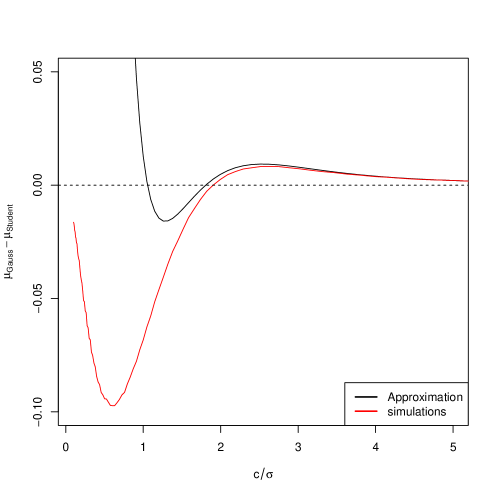
Figure 13: Large signal-to-noise ratio limit: difference of record rate between random walks with Gaussian increments and Student’s t-distributed increments. The rate was determined as the average slope $[m(200)-m(100)]/100$ (averages over $10^{5}$ samples).

References

- Andersen (1953) Andersen, Erik Sparre. 1953. “On the fluctuations of sums of random variables.” Mathematica Scandinavica 1: 263–285.
- Auer and Schuhmacher (2013a) Auer, Benjamin R, and Frank Schuhmacher. 2013a. “Performance hypothesis testing with the Sharpe ratio: The case of hedge funds.” Finance Research Letters 10 (4): 196–208.
- Auer and Schuhmacher (2013b) Auer, Benjamin R, and Frank Schuhmacher. 2013b. “Robust evidence on the similarity of Sharpe ratio and drawdown-based hedge fund performance rankings.” Journal of international financial markets, institutions and money 24: 153–165.
- Bailey and Lopez de Prado (2014) Bailey, David H, and Marcos Lopez de Prado. 2014. “The deflated sharpe ratio: Correcting for selection bias, backtest overfitting and non-normality.” Journal of Portfolio Management 40 (5): 94–107.
- Blest (2000) Blest, David C. 2000. “Rank correlation—an alternative measure.” Australian & New Zealand Journal of Statistics 42 (1): 101–111.
- Bollerslev (1987) Bollerslev, Tim. 1987. “A conditionally heteroskedastic time series model for speculative prices and rates of return.” The review of economics and statistics 542–547.
- Bouchaud and Potters (2000) Bouchaud, J.-P., and M. Potters. 2000. Theory of Financial Risks. Cambridge University Press, Cambridge.
- Challet (2015) Challet, Damien. 2015. One- and two-sample nonparametric location tests for the signal-to-noise ratio based on record statistics. Working paper, available at http://arxiv.org/abs/1502.05367.
- Christie (2005) Christie, Steve. 2005. “Is the Sharpe ratio useful in asset allocation?.” Macquarie Applied Finance Centre Research Paper .
- Dacorogna et al. (2001) Dacorogna, Michel M., Ramazan Gencay, Ulrich A. Müller, Richard B. Olsen, and Olivier V. Pictet. 2001. An Introduction to High-Frequency Finance. London: Academic Press.
- Eisler et al. (2009) Eisler, Zoltan, Janos Kertesz, Fabrizio Lillo, and Rosario N Mantegna. 2009. “Diffusive behavior and the modeling of characteristic times in limit order executions.” Quantitative Finance 9 (5): 547–563.
- Eling and Schuhmacher (2007) Eling, Martin, and Frank Schuhmacher. 2007. “Does the choice of performance measure influence the evaluation of hedge funds?.” Journal of Banking & Finance 31 (9): 2632–2647.
- Feller (2008) Feller, Willliam. 2008. An introduction to probability theory and its applications. Vol. 2. Hoboken, NJ:: John Wiley & Sons.
- Genest and Plante (2003) Genest, Christian, and Jean-François Plante. 2003. “On Blest’s measure of rank correlation.” Canadian Journal of Statistics 31 (1): 35–52.
- Jansen and De Vries (1991) Jansen, Dennis W, and Casper G De Vries. 1991. “On the frequency of large stock returns: Putting booms and busts into perspective.” The Review of Economics and Statistics 18–24.
- Jobson and Korkie (1981) Jobson, J Dave, and Bob M Korkie. 1981. “Performance hypothesis testing with the Sharpe and Treynor measures.” The Journal of Finance 36 (4): 889–908.
- Jondeau and Rockinger (2003) Jondeau, Eric, and Michael Rockinger. 2003. “Conditional volatility, skewness, and kurtosis: existence, persistence, and comovements.” Journal of Economic Dynamics and Control 27 (10): 1699–1737.
- Le Doussal and Wiese (2009) Le Doussal, Pierre, and Kay Jörg Wiese. 2009. “Driven particle in a random landscape: Disorder correlator, avalanche distribution, and extreme value statistics of records.” Physical Review E 79 (5): 051105.
- Ledoit and Wolf (2008) Ledoit, Oliver, and Michael Wolf. 2008. “Robust performance hypothesis testing with the Sharpe ratio.” Journal of Empirical Finance 15 (5): 850–859.
- Lo (2002) Lo, Andrew W. 2002. “The statistics of Sharpe ratios.” Financial Analysts Journal 58 (4): 36–52.
- Lo, MacKinlay, and Zhang (2002) Lo, Andrew W, A Craig MacKinlay, and June Zhang. 2002. “Econometric models of limit-order executions.” Journal of Financial Economics 65 (1): 31–71.
- Longin (2005) Longin, Francois. 2005. “The choice of the distribution of asset returns: How extreme value theory can help?.” Journal of Banking & Finance 29 (4): 1017–1035.
- Magdon-Ismail et al. (2003) Magdon-Ismail, Malik, Amir Atiya, Amrit Pratap, and Yaser Abu-Mostafa. 2003. “The maximum drawdown of the brownian motion.” In Computational Intelligence for Financial Engineering, 2003. Proceedings. 2003 IEEE International Conference on, 243–247. IEEE.