Application of optimal homotopy asymptotic method to nonlinear Bingham fluid dampers

Abstract

Magnetorheological fluids (MR) are stable suspensions of magnetizable microparticles, characterized by the property to change the rheological characteristics when subjected to the action of magnetic field. Together with another class of materials that change their rheological characteristics in the presence of an electric field, called electrorheological materials are known in the literature as the smart materials or controlled materials. In the absence of a magnetic field the particles in MR fluid are dispersed in the base fluid and its flow through the apertures is behaves as a Newtonian fluid having a constant shear stress. When the magnetic field is applying a MR fluid behavior change, and behaves like a Bingham fluid with a variable shear stress. Dynamic response time is an important characteristic for determining the performance of MR dampers in practical civil engineering applications. The purpose of this paper is to show how to use the Optimal Homotopy Asymptotic Method (OHAM) to solve the nonlinear differential equation of a modified Bingham model with non-viscous exponential damping. Our procedure does not depend upon small parameters and provides us with a convenient way to optimally control the convergence of the approximate solutions. OHAM is very efficient in practice ensuring a very rapid convergence of the solution after only one iteration and with a small number of step.

Keywords: MR dampers, optimal homotopy asymptotic method, auxiliary functions, optimal parameters

² University Politehnica Timişoara, Department of Mathematics, Timişoara, 300006, Romania, e-mail: remus.ene@upt.ro

³ University Politehnica Timişoara, Department of Mechanics and Strength of Materials, 300222 Timişoara, Romania, e-mail: liviu.bereteu@upt.ro

1 Introduction

Over the past decade, much attention has been given to the MR dampers for its attractive characteristics in applications of civil engineering structures including earth-quake hazard mitigation, or high strength, insensitivity to contamination, and small power requirement. Also MR fluids have attracted considerable interest due to their wide range of use in vibration dampers for vehicle suspension systems or machinery mounts, their stiffness and damping, characteristics can be adjusted very quickly by applying a suitable electric or magnetic field [1]-[4]. The magnetorheological response of MR fluids results from the polarization induced in the suspended particles by application of an external field. The interaction between the resulting induced dipoles causes the particles to form columnar structures, parallel to the applied field. These chain-like structures restrict the motion of the fluid, thereby increasing the viscous characteristics of the suspension. The mechanical energy needed to yield these chain-like structures increases as the applied field increases resulting in a field dependent yield stress [3]. Dynamic constitutive relation of MR fluids is very complicated and provided damping force is intrinsically nonlinear, so there is not a consistent recognized mechanical model for MR dampers. The mechanical model for an MR damper is often established through optimization method according to experimental data [5]-[8]. At present, there is a variety of dynamic models for MR dampers. Some models which are simple cannot effectively simulate nonlinear dynamic characteristics of MR dampers. Although there are some models which can simulate nonlinear dynamic characteristics, they are established by strong nonlinear equations having a lot of parameters which result in complicated numerical calculation. In civil engineering Bingham model are often used for emulating the dynamic behavior of MR dampers. This model is one of the most popular models have been widely used with reasonable accuracy and computational cost. The so-called Bingham model includes a variable rigid perfectly plastic element connected in parallel to a Newtonian viscosity element. This model assumes that the fluid exhibits shear stress proportional to shear rate in the post-yield region and can be expressed as [4], [6], [7], [9]:

$$\displaystyle\tau=\tau_{y}(H)\cdot sgn(\dot{\gamma})+\eta\dot{\gamma}$$ (1)

where $\tau$ is the shear stress in the fluid, $\tau_{y}$ is the yielding shear stress controlled by the applied field $H$, $\eta$ is the post-yield viscosity independent of the applied magnetic field, $\gamma$ is the shear strain rate and $sgn(\cdot)$ is the signum function. That is, the fluid is in a state of rest and behaves viscoelastically until the shear stress is greater than the critical value $\tau_{y}$, whereas it moves like a Newtonian fluid when such a critical value is exceed.

Based on this model of the rheological behavior of electrorheological fluids, Stanway et al. [5] proposed an idealized mechanical system which consists of a Coulomb friction element placed in parallel with a viscous damper. In this model, for nonzero piston velocities $\dot{x}$, the force generated by the device is given by the fluid as follows:

$$\displaystyle F(t)=f_{c}\cdot sgn(\dot{x})+c_{0}\dot{x}+f_{0}$$ (2)

where $f_{c}$ is the coefficient of the frictional force, which is related to the fluid yield stress, $c_{0}$ is the damping coefficient, $f_{0}$ denoting an offset in the force is included to account for the nonzero mean observed in the measured force due to the presence of the accumulator. We remark that if at any point the velocity of the piston is zero, the force generated in the frictional element is equal to the applied force. The Bingham model accounts for electro- and magneto- rheological fluid behavior beyond the yield point, i.e. for fully developed fluid flow or sufficiently higher shear rates. However, it assumes that the fluid remains rigid in the pre-yield region [4]. This the Bingham model does not describe the fluid’s elastic properties at small deformations and low shear rates which is necessary for dynamic applications. Lee and Wereley [10] and Wang and Gordaninejad [11] employed the Herschel-Bulkley model to accomodate fluid post-yield shear thinning and shear thickening. In this model, the constant post-yield plastic viscosity in the Bingham model is replaced with a power law model dependent on the shear strain rate. However due to its simplicity, the Bingham model is still very effective, especially in the damper design phase [9]. The Herschel-Bulkley model can be expressed by

$$\displaystyle\tau=\left[\tau_{y}(H)\cdot sgn(\dot{\gamma})+k\left(\dot{\gamma}\right)^{\frac{1}{m}}\right]sgn(\dot{\gamma})$$ (3)

where $k$ is the consistency parameter and $m$ is fluid behavior index of the magnetorheological fluid. For $m>1$, Eq. (3) represents a shear thinning fluid while shear thickening fluids are described by $m<1$. For $m=1$, the Herschel-Bulkley model reduces to the Bingham model [12]. Zubieta et al. [13] have proposed field-dependent plastic models, for magnetorheological fluid based on the original Bingham plastic and Herschel-Bulkley plastic models. In the field dependent Bingham and Herschel-Bulkley model, the rheological properties of magnetorheological fluid depend applied magnetic field and can be estimated by the following equation [12]:

$$\displaystyle Y=Y_{\infty}+(Y_{0}-Y_{\infty})\left(2e^{-B\alpha_{{}_{YS}}}-e^{-2B\alpha_{{}_{YS}}}\right)$$ (4)

where $Y$ stands for a rheological parameters of magnetorheological fluid such as yield stress, post-yield viscosity, fluid consistency and flow behavior index. The value of parameter $Y$ tends from the zero applied field value $Y_{0}$ to the saturation value $Y_{\infty}$ and $\alpha_{{}_{YS}}$ is the saturation moment index of the $Y$ parameter, $B$ is the applied magnetic density. The value of $Y_{0}$, $Y_{\infty}$ and $\alpha_{{}_{YS}}$ are determined from experimental results using curve fitting method.

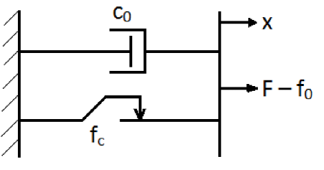
Figure 1: Bingham model

The Bingham body model, presented in Fig. 2 differs from the Bingham model (Fig. 1) by the introducing of a spring $k$. The Bingham body model contains in parallel three elements that is connecting the elements of St. Venant, Newton and the element of Hooke. To a certain value of the applied force $f_{c}$ - static friction force of the St. Venant element, only the spring will deform, similarly to the elastic Hooke body.

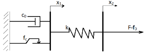
Figure 2: Bingham body model

If this force is greater than $f_{c}$ the Bingham body will elongate. The rate of the deformation will be proportional to the difference of the applied force and the friction force of the St. Venant element [14]. In theis case the damping force $F$ can be expressed as

$$\displaystyle F(t)=\left\{\begin{array}[]{lll}f_{c}sgn(\dot{x}_{1})+c_{0}\dot{x}_{1}+f_{0}&\textrm{for}&|F|>f_{c}\\ k(x_{2}-x_{1})+f_{0}&\textrm{for}&|F|\leq f_{c}\\ \end{array}\right.$$ (7)

where $k$ is the stiffness of the elastic body (Hooke model) and the other parameters have the same meaning as in Eq. (2).

An extension of the Bingham model is formulated by Gamota and Filisko [15]. This extension describes the electrorheological fluid behavior in the pre-yield and post-yield region as well as the yield point. This viscoelastic-plastic model depends on connection of the Bingham, Kelvin-Voight body and Hooke body models (Fig. 3).

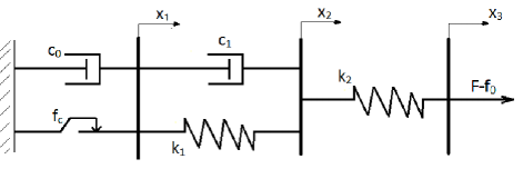
Figure 3: Extended Bingham model for the Gamota-Filisko model

The damping force in the Gamota-Filisko model is given by

$$\displaystyle F(t)=\left\{\begin{array}[]{llll}k_{1}(x_{2}-x_{1})+c_{1}(\dot{x}_{2}-\dot{x}_{1})+f_{0}&=c_{0}\dot{x}_{1}+f_{c}sgn(\dot{x}_{1})+f_{0}=\\ &=k_{2}(x_{3}-x_{2})+f_{0}\ \ \textrm{for}\ |F|>f_{c}\\ k(x_{2}-x_{1})+c_{1}\dot{x}_{2}+f_{0}&=k_{2}(x_{3}-x_{2})+f_{0}\ \ \textrm{for}\ |F|\leq f_{c}\\ \end{array}\right.$$ (11)

where $c_{0}$, $f_{0}$ and $f_{c}$ are known from Bingham model (2) and the parameters $c_{1}$, $k_{1}$ and $k_{2}$ are associated with the fluid’s elastic properties in the pre-yield region. We remark that if $|F|\leq f_{c}$ then $\dot{x}_{1}=0$, which means that when the friction force $f_{c}$ related with the new stress in the fluid is greater than the damping force $F$, the piston remain motionless. Another view of visco-elastic-plastic properties of MR damper behavior is proposed by Li et al. [16]. In essence the damping force is equal to the visco-plastic force, to which besides the friction force connected with the fluid shear stress $f_{c}$, the viscotic force and inertial force contribute, which can be written in the form [14]

$$\displaystyle F(t)=f_{c}\cdot sgn(\dot{x})+c_{0}\dot{x}+m\ddot{x}$$ (12)

where $c_{0}$ is a co-factor of viscotic friction and $m$ is the mass of replaced MR fluid dependent on the amplitude and frequency of a kinematic excitation applied to the piston.

A discrete element model with similar components, referred to as the BingMax model, is reviewed by Makris et al. [17]. It consists of a Maxwell element in parallel with a Coulomb friction element as depicted in Fig 4.

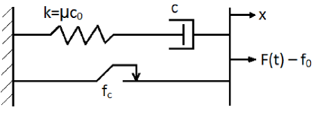
Figure 4: BingMax model

The force $F(t)$ is given by

$$\displaystyle F(t)=c\cdot\int_{0}^{t}\mu e^{-\mu(t-\tau)}\dot{x}(\tau)\ d\tau+f_{c}sgn(\dot{x}(t))$$ (13)

where $\mu$ is a parameter meaning the non-viscous damping effect (or the relaxation parameter [18]). The model for the damping force expressed as

$$\displaystyle f_{d}(t)=c\cdot\int_{0}^{t}\mu e^{-\mu(t-\tau)}\dot{x}(\tau)\ d\tau$$ (14)

was originally proposed by Biot [19] and later used by several authors in the context of dynamics of viscoelastic systems. Eq. (14) physically implies that the previous time histories of the velocity $\dot{x}$ contribute to the current damping force and the most recent instances of velocity have the highest influence. In the limiting case when $\mu\rightarrow\infty$, the exponential kernel function approaches the Dirac delta function $\delta(t)$. For this special case damping force given by (14) reduces to the case of viscous damping. For viscoelastic systems, an equation similar to Eq. (14) is often associated with the stiffness parameter. Cremer and Heckl [20] concluded that: ”of the many after-effect functions, that are possible in principle, one - the so-called relaxation function - is physically meaningful”.

Based on the above considerations, in what follows we consider the behavior of a magnetorheological damper after Bingham models which in addition contains a nonlinear term.

The motion equation is established in the form:

$$\displaystyle m\frac{d^{2}x(\bar{t})}{d\bar{t}^{2}}+\bar{c}\cdot\int_{0}^{\bar{t}}\bar{\mu}e^{-\bar{\mu}(\bar{t}-\bar{\tau})}\dot{x}(\bar{\tau})\ d\bar{\tau}+kx(\bar{t})+\alpha kx^{3}(\bar{t})+$$

$$+k\beta sgn(\dot{x}(\bar{t}))+kf_{0}=0$$ (15)

where $m$, $\bar{c}$, $\bar{\mu}$, $k$, $\alpha k$, $\beta k$ and $kf_{0}$ are mass, damping relaxation, linear stiffness, nonlinear stiffness, coefficient of frictional force and offset of the force, respectively; $x$, $\dot{x}$ and $\ddot{x}$ are the dynamic responses of the structure (displacement, velocity and acceleration).

The initial conditions are:

$$\displaystyle x(0)=A,\ \ \ \dot{x}(0)=v_{0}\cdot\sqrt{\frac{k}{m}}$$ (16)

The objective of the present paper is to propose an accurate procedure to nonlinear differential equation of the nonlinear Bingham model given by Eq. (1), using OHAM. A version of the OHAM is applied in this study to derive highly accurate analytical expressions of the solutions using only one iteration and a small number of steps. Our procedure is independent of the presence of any small or large parameters, contradistinguishing from other known methods in literature. The main advantage of this approach is the control of the convergence of approximate solutions in a very rigorous way. A very good agreement was found between our approximate solutions and numerical results, which proves that our method is very efficient and accurate.

2 Basic ideas of the optimal homotopy asymptotic method

Eq. (1) with initial conditions (16) can be written in a more general form

$$\displaystyle N\left[x(t)\right]=0$$ (17)

where $N$ is a given nonlinear differential operator depending on the unknown function $x(t)$, subject to the initial conditions

$$\displaystyle B\left(x(t),\ \frac{dx(t)}{dt}\right)=0.$$ (18)

Let $x_{0}(t)$ be an initial approximation of $x(t)$ and $L$ an arbitrary linear operator such as

$$\displaystyle L\left[x_{0}(t)\right]=0,\ \ B\left(x_{0}(t),\ \frac{dx_{0}(t)}{dt}\right)=0.$$ (19)

It should be emphasize that this linear operator $L$ is not unique.

If $p\in[0,\ 1]$ denotes an embedding parameter and $X$ is an analytic function, then we propose to construct a homotopy [21] - [26]:

$$\displaystyle\mathcal{H}\left[L\left(X(t,p)\right),\ H(t,C_{i}),\ N\left(X(t,p)\right)\right],\ \ i=1,2,...,s$$ (20)

with properties

$$\displaystyle\mathcal{H}\left[L\left(X(t,0)\right),\ H(t,C_{i}),\ N\left(X(t,0)\right)\right]=L\left(X(t,0)\right)=L\left(x_{0}(t)\right)=0$$ (21)

$$\displaystyle\mathcal{H}\left[L\left(X(t,1)\right),\ H(t,C_{i}),\ N\left(X(t,1)\right)\right]=H(t,C_{i})N\left(x(t)\right)=0,$$ (22)

$$i=1,2,...,s$$

where $H(t,C_{i})\neq 0$, is an arbitrary auxiliary convergence-control function depending on variable $t$ and on $s$ arbitrary parameters $C_{1}$, $C_{2}$, …, $C_{s}$ unknown now and will be determined later.

Let us consider the function $X$ in the form

$$\displaystyle X(t,p)=x_{0}(t)+px_{1}(t,C_{i}).$$ (23)

By substituting Eq. (23) into equation obtained by means of homotopy (20)

$$\displaystyle\mathcal{H}\left[L\left(X(t,p)\right),\ H(t,C_{i}),\ N\left(X(t,p)\right)\right]=0,\ \ i=1,...,s$$ (24)

and then equating the coefficients of $p^{0}$ and $p^{1}$, we obtain

$$\displaystyle\mathcal{H}\left[L\left(X(t,p)\right),\ H(t,C_{i}),\ N\left(X(t,p)\right)\right]=$$

$$\displaystyle=L\left(x_{0}(t)\right)+p\left[L\left(x_{1}(t,C_{i})\right)-L\left(x_{0}(t)\right)-H(t,C_{i})N\left(x_{0}(t)\right)\right]=0,$$ (25)

$$i=1,2,...,s.$$

From the last equation, we obtain the governing equation of $x_{0}(t)$ given by Eq. (19) and the governing equation of $x_{1}(t,C_{i})$, i.e.:

$$\displaystyle L\left(x_{1}(t,C_{i})\right)=H(t,C_{i})N\left(x_{0}(t)\right),\ \ \ B\left(x_{1}(t,C_{i}),\ \frac{dx_{1}(t,C_{i})}{dt}\right)=0,$$ (26)

$$i=1,\ ...,\ s$$

where we find the following expression for the nonlinear operator:

$$\displaystyle N\left(x_{0}(t)\right)=\sum_{i=1}^{m}h_{i}(t)g_{i}(t)$$ (27)

In the Eq. (27) the functions $h_{i}(t)$ and $g_{i}(t)$, $i=1,\ ...,\ m$ are known and depend on the initial approximation $x_{0}(t)$ and also on the nonlinear operator, $m$ being a known integer number.

In this way, taking into account Eq. (22), from Eq. (23) for $p=1$, we obtain the first-order approximate solution which becomes

$$\displaystyle\overline{x}(t,C_{i})=x_{0}(t)+x_{1}(t,C_{i}),\ \ \ i=1,\ ...,\ s$$ (28)

It should be emphasized that $x_{0}(t)$ and $x_{1}(t,C_{i})$ are governed by the linear Eqs. (19) and (26) respectively with initial / boundary conditions that come from the original problem. It is known that the general solution of nonhomogeneous linear Eq. (26) is equal to the sum of general solution of the corresponding homogeneous equation and of some particular solutions of the nonhomogeneous equation. However, the particular solutions are readily selected only in the exceptional cases.

In what follows we do not solve Eq. (26), but from the theory of differential equations, taking into considerations the method of variation of parameters, Cauchy method, method of influence function, the operator method and so on, is more convenient to consider the unknown function $x_{1}(t,C_{i})$, in the form

$$\displaystyle x_{1}(t,C_{j})=\sum_{i=1}^{n}H_{i}(t,h_{j}(t),C_{j})g_{i}(t),\ \ \ j=1,\ ...,\ s$$ (29)

$$\displaystyle B\left(x_{1}(t,C_{i}),\ \frac{dx_{1}(t,C_{i})}{dt}\right)=0$$

where within expression of $H_{i}(t,h_{j}(t),C_{j})$ appear combinations of some functions $h_{j}$, the some terms which are given by the corresponding homogeneous equation and the unknown parameters $C_{j}$, $j=1,\ ...,\ s$. In the sum given by Eq. (29) appear an arbitrary number of $n$ of the such terms.

We have a large freedom to choose the value of $n$. We cannot demand that $x_{1}(t,C_{i})$ to be solutions of Eq. (26) but $\overline{x}(t,C_{i})$ given by Eq. (28) with $x_{1}(t,C_{i})$ given by Eq. (29), are the solutions of the Eq. (17). This is underlying idea of our method. The convergence of the approximate solution $\overline{x}(t,C_{i})$ given by Eq. (28) depends upon the auxiliary functions $H_{i}(t,h_{i},C_{j})$, $j=1,\ ...,\ s$. There are many possibilities to choose these functions $H_{i}$. We try to choose the auxiliary functions $H_{i}$ so that within Eq. (29) the term $\sum_{i=1}^{n}H_{i}(t,h_{j}(t),C_{j})g_{i}(t)$ be of the same shape with the term $\sum_{i=1}^{m}h_{i}(t)g_{i}(t)$ given by Eq. (27). The first-order approximate solution $\overline{x}(t,C_{i})$ also depend on the parameters $C_{j}$, $j=1,\ ...,\ s$. The values of these parameters can be optimally identified via various methods, such as: the least-square method, the Galerkin method the collocation method, the Ritz method or minimizing the square residual error:

$$\displaystyle J(C_{1},C_{2},...,C_{s})=\int_{D}R^{2}(t,C_{1},C_{2},...,C_{s})\ dt$$ (30)

where the residual $R$ is given by

$$\displaystyle R(t,C_{1},C_{2},...,C_{s})=N\left(\overline{x}(t,C_{i})\right).$$ (31)

The unknown parameters $C_{1},\ C_{2},\ ...,\ C_{s}$ can be identified from the conditions:

$$\displaystyle\frac{\partial J}{\partial C_{1}}\ =\ \frac{\partial J}{\partial C_{2}}\ =\ ...\ =\ \frac{\partial J}{\partial C_{s}}=\ 0.$$ (32)

With these parameters known (called optimal convergence-control parameters), the first-order approximate solution given by Eq. (28) is well-known.

It should be emphasized that our procedure contains the auxiliary functions $H_{i}(t,f_{i},C_{j})$, $i=1,\ ...,\ m$, $j=1,\ ...,\ s$ which provides us with a simple way to adjust and control the convergence of the approximate solutions. It is very important to properly choose these functions $H_{i}(t,f_{i},C_{j})$ which appear in the construction in the first-order approximation.

3 Application of OHAM to nonlinear Bingham fluid dampers

In what follows, we apply our procedure to obtain approximate solution of Eqs. (1) and (16). For this purpose, we introduce the dimensionless variables

$$\displaystyle t=\bar{t}\sqrt{\frac{m}{k}},\ \ \ \tau=\bar{\tau}\sqrt{\frac{m}{k}}$$ (33)

such that Eq. (1) can be expressed as

$$\displaystyle\ddot{x}(t)+2c\cdot\int_{0}^{t}\mu e^{-\mu(t-\tau)}\dot{x}(\tau)\ d\tau+x(t)+\alpha x^{3}(t)+\beta sgn(\dot{x}(t))+f_{0}=0$$ (34)

where $c=\frac{\bar{c}}{2\sqrt{km}}$ $\mu=\sqrt{\frac{m}{k}}\bar{\mu}$ and the overdot represents differentiation with respect to dimensionless time. The initial conditions (16) become

$$\displaystyle x(0)=A,\ \ \ \dot{x}(0)=v_{0}$$ (35)

Making the transformation

$$\displaystyle x(t)=Ae^{-\lambda t}z(t)$$ (36)

where $\lambda$ is an unknown parameter at this moment, Eq. (34) can be written as

$$\displaystyle\ddot{z}-2\lambda\dot{z}+(\lambda^{2}+2\mu c+1)z-2c\mu^{2}\cdot\int_{0}^{t}e^{(\lambda-\mu)(t-\tau)}z(\tau)\ d\tau+$$

$$+\alpha A^{2}e^{-2\lambda t}z^{3}+\frac{\beta}{A}e^{\lambda t}sgn(\dot{z}-\lambda z)+\frac{f_{0}e^{\lambda t}}{A}-2c\mu e^{(\lambda-\mu)t}=0$$ (37)

The initial conditions (35) become

$$\displaystyle z(0)=1,\ \ \ \dot{z}(0)=\lambda+\frac{v_{0}}{A}$$ (38)

For the nonlinear differential equation (3), we choose the linear operator of the form:

$$\displaystyle L\left(z(t)\right)=\ddot{z}(t)+\omega^{2}z(t)$$ (39)

where $\omega$ is unknown parameter.

The nonlinear operator corresponding to Eqs. (3) and (39) is

$$\displaystyle N\left(z(t)\right)=-2\lambda\dot{z}+(\lambda^{2}+2\mu c+1-\omega^{2})z-2c\mu^{2}\cdot\int_{0}^{t}e^{(\lambda-\mu)(t-\tau)}z(\tau)\ d\tau+$$

$$+\alpha A^{2}e^{-2\lambda t}z^{3}+\frac{\beta}{A}e^{\lambda t}sgn(\dot{z}-\lambda z)+\frac{f_{0}}{A}e^{\lambda t}-2c\mu e^{(\lambda-\mu)t}\qquad$$ (40)

The initial approximation $z_{0}(t)$ can be obtained from Eq. (19) with initial / boundary conditions:

$$\displaystyle z_{0}(0)=1,\ \ \ \dot{z}_{0}(0)=-\frac{\omega^{2}}{\lambda}$$ (41)

Eq. (19) with the linear operator (39) and with initial / boundary conditions (41) has the solution

$$\displaystyle z_{0}(t)=\cos\omega t-\frac{\omega}{\lambda}\sin\omega t$$ (42)

The nonlinear operator corresponding to Eq. (27) it holds that

$$\displaystyle N\left(z_{0}(t)\right)=\frac{\lambda(1+\lambda^{2}+\omega^{2}+2\mu c)-2\mu^{2}c(\omega^{2}-\lambda^{2}+\lambda\mu)}{\lambda(\omega^{2}+(\mu-\lambda)^{2})}\cos\omega t+$$

$$+\frac{\omega(\lambda^{2}+\omega^{2}-2\mu c-1)(\lambda^{2}+\omega^{2}+\lambda^{2}-2\mu\lambda)+2\mu^{2}c\omega(\mu-2\lambda)}{\lambda(\omega^{2}+(\mu-\lambda)^{2})}\sin\omega t+$$

$$+\frac{2\mu^{2}c(\omega^{2}-\lambda^{2})-2\mu c\lambda(\omega^{2}+\lambda^{2}-2\lambda\mu)}{\lambda(\omega^{2}+(\mu-\lambda)^{2})}e^{(\lambda-\mu)t}+\frac{f_{0}}{A}e^{\lambda t}+$$

$$+\frac{\alpha A^{2}}{4}e^{-2\lambda t}\left[\frac{3(\omega^{2}+\lambda^{2})}{\lambda^{2}}\cos\omega t+\frac{3\omega(\omega^{2}+\lambda^{2})}{\lambda^{3}}\sin\omega t+\frac{\lambda^{2}-3\omega^{2}}{\lambda^{2}}\cos 3\omega t+\right.$$

$$\left.+\frac{\omega(\omega^{2}-3\lambda^{2})}{\lambda^{3}}\sin 3\omega t\right]-\frac{4\beta}{\lambda A}e^{\lambda t}\left(\cos\omega t-\frac{1}{3}\cos 3\omega t+\frac{1}{5}\cos 5\omega t-\right.$$

$$\left.-\frac{1}{7}\cos 7\omega t+\frac{1}{9}\cos 9\omega t-...\right)\qquad$$ (43)

From Eqs. (3), (38) and (29), we choose

$$\displaystyle z_{1}(t)=C_{1}t^{2}\cos\omega t+(C_{2}t^{2}+C_{3}t)\sin\omega t+$$

$$+\left[\left(C_{4}t^{2}+(v_{0}+\frac{\omega^{2}+\lambda^{2}}{\lambda}A+3\lambda C_{7})t\right)\cos 3\omega t+\right.$$

$$\left.+(C_{5}t^{2}+C_{6}t)\sin 3\omega t+C_{7}\right]e^{-2\lambda t}-C_{7}e^{\lambda t}\cos\omega t$$ (44)

The first-order approximate solution of Eqs. (34) and (35) given by Eq. (28) is obtained from Eqs. (42), (3) and (36):

$$\displaystyle x(t)=\left[(C_{1}t^{2}+A)\cos\omega t+(C_{2}t^{2}+C_{3}t-\frac{\omega}{\lambda}A)\sin\omega t\right]e^{-\lambda t}+$$

$$+\left\{\left[C_{4}t^{2}+\left(\Big{(}v_{0}+\frac{\omega^{2}+\lambda^{2}}{\lambda}\Big{)}A+3\lambda C_{7}\right)t\right]\cos 3\omega t+\right.$$

$$\left.+(C_{5}t^{2}+C_{6}t)\sin 3\omega t+C_{7}\right\}e^{-3\lambda t}-C_{7}\cos\omega t$$ (45)

4 Numerical results

We illustrate the accuracy of our procedure for the following values of the parameters: $c=0.1$, $\mu=20$, $\alpha=1$, $\beta=0.1$, $f_{0}=0.1$ $A=5$, $v_{0}=0.1$. The optimal convergence-control parameters are determined by means of the least-square method in the three steps as follows:

For $t\in[0,\ 7/2]$ we obtain

$$C_{1}=-8.3835528344,\ C_{2}=0.4059363155,\ C_{3}=9.8101433224,$$

$$C_{4}=12.7300955924,\ C_{5}=-8.3640772984,\ C_{6}=-14.6926248464,$$

$$C_{7}=-15.2775231617,\ \lambda=0.4221369200,\ \omega=1.1700000000.$$

The first-order approximate solution given by Eq. (3) becomes for this first step:

$$\displaystyle\bar{x}(t)=\left[(-8.3835528344t^{2}+5)\cos\omega t+(0.4059363155t^{2}+9.8101433224t-\right.$$

$$\left.-13.8580629241)\sin\omega t\right]e^{-0.4221369200t}+\left[(12.7300955924t^{2}-\right.$$

$$-1.0230014969t)\cos 3\omega t+(-8.3640772984t^{2}-14.692624846t)\sin 3\omega t-$$

$$\left.-15.2775231617\right]e^{-1.2664107600t}+15.2775231617\cos\omega t\qquad$$ (46)

For the second step, when $t\in[7/2,\ 7]$ we obtain

$$\displaystyle\bar{x}(t)=\left[(-18.7159298670t^{2}+1.3931962652)\cos\omega t+(2.5809325241t^{2}-\right.$$

$$\left.-12.3307330274t-7.2827523763)\sin\omega t\right]e^{-0.3726878974t}+\left[(16.1687136688t^{2}-\right.$$

$$-76.6284415838t)\cos 3\omega t+(1.8324463202t^{2}-15.4843220143t)\sin 3\omega t-$$

$$\left.-68.7655829044\right]e^{-1.1180636924t}+68.7655829044\cos\omega t\qquad$$ (47)

where $\omega=1.9481775386$, $\lambda=0.3726878974$.

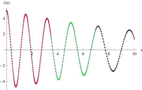
Figure 5: Comparison between the approximate solution (4), (4) and (4) and numerical solution: —– numerical solution; ……… approximate solution

In the last case, when $t\in[7,\ 10]$, the first-order approximate solution is

$$\displaystyle\bar{x}(t)=\left[(0.1521594849t^{2}+2.6425574994)\cos\omega t+(-1.4223903751t^{2}+\right.$$

$$\left.+13.8451447750t-10.3560770110)\sin\omega t\right]e^{-0.1870115667t}+\left[(-7.9954565850t^{2}+\right.$$

$$+12.3657070213t)\cos 3\omega t+(1.5073646864t^{2}-0.3337501284t)\sin 3\omega t+$$

$$\left.+1.1037184321\right]e^{-0.5610347000t}-1.1037184321\cos\omega t\qquad$$ (48)

where $\omega=0.7328908403$, $\lambda=0.1870115667$.

In Fig. 5 is plotted a comparison between the first-order approximate solution and numerical results.

It can be seen that the solution obtained by the proposed procedure are nearly identical with the numerical solution obtained using a fourth-order Runge-Kutta method.

5 Conclusions

The Optimal Homotopy Asymptotic Method is employed to propose an analytic approximate solutions for the nonlinear Bingham model. Our procedure is valid even if the nonlinear differential equation does not contain any small or large parameters. In construction of the homotopy appear some distinctive concepts as: the linear operator, the nonlinear operator, the auxiliary functions $H_{i}(t,C_{i})$ and several optimal convergence-control parameters $\lambda$, $\omega$, $C_{1}$, $C_{2}$, … which ensure a fast convergence of the solutions. The example presented in this work, leads to the conclusion that the obtained results are of very accurate using only one iteration and three steps. The OHAM provides us with a simple and rigorous way to control and adjust the convergence of the solution through the auxiliary functions $H_{i}(t,C_{i})$ involving several parameters $\lambda$, $\omega$, $C_{1}$, $C_{2}$, … which are optimally determined. Actually, the capital strength of OHAM is its fast convergence, which proves that our procedure is very efficient in practice.

Conflict of Interests
The authors declare that there is no conflict of interests regarding the publication of this paper.

References

- [1] W. I. Kordonsky, Magneto-rheological fluids and their applications, Mater. Technol., 8(11), 1993, 240–242.
- [2] O. Ashour, A. Craig, Magneto-rheological fluids: materials, characterization and devices, J. Int. Mater. Syst. Struct., 7, 1996, 123–130.
- [3] M. R. Jolly, J. W. Bender, J. D. Carlson, Properties and Applications of Commercial Magnetorheological Fluids, SPIE 5 Annual Int. Symposium on Smart Structures and Materials, San Diego CA, 15 March 1998.
- [4] T. Butz, O. Von Stryk Modelling and Simulation of ER and MR Fluid Dampers, ZAMM, Z. Angew. Math. Mech. 78, 1998, 1–22.
- [5] R. Stanway, J. L. Sproston, N. G. Stevens, Non-linear modelling of an electro-rheological vibration damper, Journal of Electrostatics, 20(2), 1987, 167–184.
- [6] J. D. Carlson, M. R. Jolly, MR fluid, foam and elastomer devices, Mechatronics, 10, 2000, 555-564.
- [7] B. F. Spencer, S. J. Dyke, M. K. Sain, J. D. Carlson, Phenomenological model for magnetorheological dampers, Journal of Engineering Mechanics, 123(3), 1997, 230–238.
- [8] C. Li, Q. Liu, S. Lan, Application of Support Vector Machine - Based Semiactive Control for Seismic Protection of Structures with Magnetorheological Dampers, Mathematical Problems in Engineering, 2012, Article ID 268938, 18 pages.
- [9] G. Yang, B. F. Spencer Jr., J. D. Carlson, M. K. Sain, Large-scale MR fluid dampers: modelling and dynamic performance considerations, Engineering Structures, 24(3), 2002, 309–323.
- [10] D. Y. Lee, N. M. Wereley, Analysis of electro- and magneto-rheological flow mode dampers using Herschel-Bulkley model, Proceedings of SPIE Smart Structure and Materials Conferince, Vol. 3989 Newport Beach, California 2000, 244–252.
- [11] X. Wang, F. Gordaninejad Study of field-controllable, electro- and magneto- rheological fluid dampers in flow mode using Herschel-Bulkley theory, Proceedings of SPIE Smart Structure and Materials Conferince, Vol. 3989 Newport Beach, California 2000, 232–243.
- [12] Q.-H. Nguyen, S.-B. Choi Optimal Design Methodology of Magnetorheological Fluid Based Mechanisms, Chap. 14 from Smart Actuation and Sensing Systems-Recent Advances and Future Challenges, INTECH 2012, http://dx.doi.org/10.5772/51078.
- [13] M. Zubieta, S. Eceolaza, M. J. Elejabarrieta, M. Bou-Ali, Magnetorheological fluids: characterization and modelling of magnetization, Smart Mater. Struct., 18, 2009.
- [14] B. Sapiński, J. Filuś, Analysis of parametric models of MR linear damper, Journal of Theoretical and Applied Mechanics, 41(2), 2003, 215–240.
- [15] D. R. Gamota, F. E. Filisko, Dynamic mechanical studies of electrorheological materials: Moderate frequency, Journal of Rheology, 35, 1991, 399–425.
- [16] W. H. Li, G. Z. Yao, G. Chen, S. H. Yeo, F. F. Yap, Testing and steady state modelling of a linear MR damper under sinusoidal loading, Smart Mater. Struct., 9, 2000, 95–102.
- [17] N. Makris, S. A. Burton, D. P. Taylor Electrorheological damper with annular ducts for seismic protection applications, Smart Mater. Struct., 5, 1996, 551–564.
- [18] S. Adhikari, Structural Dynamic Analysis with Generalized Damping Models, Wiley, 2014.
- [19] M. A. Biot, Linear thermodynamics and the mechanics of solids, Proceedings of the Third U. S. National Congress on Applied Mechanics, 1958, 1–18.
- [20] L. Cremer, M. Heckl Structure-borne Sound, Springer, Berlin, 1973.
- [21] V. Marinca, N. Herişanu, C. Bota, B. Marinca, An optimal homotopy asymptotic method applied to the steady flow of a fourth grade fluid past a porous plate, Applied Mathematics Letters, 22, 2009, 245–251.
- [22] V. Marinca, N. Herişanu, Nonlinear Dynamical Systems in Engineering - Some Approximate Approaches, Springer Verlag, Heidelberg, 2011.
- [23] V. Marinca, R.-D. Ene, Analytical approximate solutions to the Thomas-Fermi equation, Central Eur. J. of Physics, 12(7), 2014, 503–510.
- [24] V. Marinca, R.-D. Ene, Dual approximate solutions of the unsteady viscous flow over a shrinking cylinder with Optimal Homotopy Asymptotic Method, Advances in Mathematical Physics, 2014, Article ID 417643, 11 pages.
- [25] V. Marinca, R.-D. Ene, B. Marinca, Analytic approximate solution for Falkner-Skan equation, The Scientific World Journal, 2014, Article ID 617453, 22 pages.
- [26] V. Marinca, R.-D. Ene, B. Marinca, R. Negrea Different approximations to the solution of upper-convected Maxwell fluid over of a porous stretching plate, Abstract and Applied Analysis, 2014, Article ID 139314, 13 pages.