Bifurcation of plane-to-plane map-germs with corank two of parabolic type

Abstract.

There is a unique $\mathcal{A}$-moduli stratum of plane-to-plane germs which forms an open dense subset in the $\mathcal{K}$-orbit of $I_{2,3}:(x^{2}+y^{3},xy)$. We describe explicitly the bifurcation diagram of its topologically $\mathcal{A}_{e}$-versal unfolding. Two geometric applications to parabolic crosscaps and parabolic umbilic are presented.

1. Introduction

The bifurcation diagram of a family of smooth functions or mappings takes a fundamental role in Catastrophe Theory – by definition it is the locus in the parameter space at which the corresponding function fails to be structurally stable; Along the locus, qualitative changes of the function occur. In this paper, we deal with generic families of plane-to-plane maps with at most $3$-parameters within the $\mathcal{A}$-classification theory ($\mathcal{A}$ denotes the equivalence of map-germs via the action of diffeomerphism-germs of source and target).

Bifurcation diagrams for $\mathcal{A}$-types of corank one germs can be found in several literatures; Arnold-Platonova [1, 2], Rieger [21, 22], Gibson-Hobbs [9] and Aicardi-Ohmoto [16]. In contrast, for corank two germs (Table 1 below), there had been very few known diagrams until quite recently. The case of deltoid is easy, while other cases may require a lot of computations; The bifurcation diagrams for types sharksfin and odd-shaped sharksfin were first presented rigorously in [28, 29], that will partly be summarized in §3 (Fig.4, 5). The remaining case in codimension $3$ is the $\mathcal{A}$-moduli stratum in the $\mathcal{K}$-orbit of the germ $I_{2,3}:(x^{2}+y^{3},xy)$; the $\mathcal{K}$-orbit has a unique topological $\mathcal{A}$-type (Rieger-Ruas [23], Gaffney-Mond [8]).

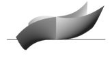
Figure 1. Apparent contour of $I_{2,3}$ and projection of parabolic crosscap

Our main purpose is to compute and describe explicitly its bifurcation diagram in the same way as [28, 29] (Theorem 3.1 and Fig.7). Note that the structure of nearby $\mathcal{K}$-orbits has been known in 70’s by Lander [14, §5.5]. In this paper we go further to find the finer structure of local and multi-$\mathcal{A}$-types appearing in the topologically $\mathcal{A}_{e}$-versal unfolding of type $I_{2,3}$.

$$\begin{array}[]{c| l | l }\mbox{cod}&\;\;\mbox{type}&\;\;\mbox{normal form}\\ \hline\cr\hline\cr 2&I_{2,2}^{1,1}\,(\mbox{sharksfin})&(x^{2}+y^{3},y^{2}+x^{3})\\ &II_{2,2}^{1,1}\,(\mbox{deltoid})&(x^{2}-y^{2}+x^{3},xy)\\ \hline\cr 3&I_{2,2}^{2,1}\,(\mbox{odd-shaped sharksfin})&(x^{2}+y^{5},y^{2}+x^{3})\\ &I_{2,3}\,(\mbox{$\mathcal{A}$-moduli})&(x^{2}+y^{3}+\alpha xy^{2}+\beta y^{4}+\cdots,xy)\\ \end{array}$$

Table 1. Corank two germs with $\mathcal{A}_{e}$-codim. $\leq 3$.

In the last half of this paper, we discuss applications to ‘parabolic objects’ in several geometric settings. The key idea of our approach is as follows: We first reformulate the problem in terms of $\mathcal{A}$-singularity types arising in some family of plane-to-plane maps naturally associated to the setting, and then embed the family into our $C^{0}$-versal unfolding of $I_{2,3}$. That may yield a $2$-dimensional section of our bifurcation diagram in the parameter $3$-space, from which one can deduce some topological nature of bifurcations of the parabolic object under consideration. For instance, the germ of type $I_{2,3}$ naturally appears in the parallel projection of a parabolic crosscap to the plane along the tangent line at the crosscap point (Fig.1, right). Our result provides a new insight into differential geometry of parabolic crosscaps in $\mathbb{R}^{3}$ (cf. Nuño-Ballesteros and Tari [15], Oliver [17]). In geometric optics or symplectic geometry, the singularity of $I_{2,3}$ is realized as a planar caustics of parabolic umbilic type $D_{5}$, which is one of most favorite singularities in R. Thom [27]. In Appendix, we apply our result to this setting and discuss generic $2$-parameter ‘perestroikas’ of planar caustics.

The authors thank the organizers of Japanese-Brazilian workshop on singularities (RIMS, 2013); it was a nice opportunity to discuss the problem dealt in this paper with several experts. The third author is partly supported by JSPS grant no.23654028.

2. Recognition of $\mathcal{A}$-types of corank one germs

2.1. $\mathcal{A}$-classification

$C^{\infty}$ map-germs $f,g:\mathbb{R}^{2},0\to\mathbb{R}^{2},0$ are $\mathcal{A}$-equivalent if there is a pair $(\sigma,\tau)$ of diffeomorphism germs of source and target planes at the origins so that $g=\tau\circ f\circ\sigma^{-1}$. We say $f$ is $\mathcal{A}$-simple if the cardinality of nearby $\mathcal{A}$-orbits is finite (otherwise, $f$ belongs to an $\mathcal{A}$-modulus, i.e., some continuous family of $\mathcal{A}$-orbits). The corank of $f$ means $\dim\ker df(0)$. Let $T\mathcal{A}_{e}.f$ denote the extended $\mathcal{A}$-tangent space of $f$, then the $\mathcal{A}_{e}$-codimension of $f$ is defined by $\dim_{\mathbb{R}}\theta(f)/T\mathcal{A}_{e}.f$; that is the smallest number of parameters required for constructing its $\mathcal{A}_{e}$-versal unfolding (such an unfolding is called to be ($\mathcal{A}_{e}$-)miniversal). Equivalently, a singularity type of $\mathcal{A}_{e}$-codimension $\leq r$ means that it generically appears in $r$-parameter families of maps. In particular, $f$ is a stable germ if and only if its $\mathcal{A}_{e}$-codimension is $0$. As for the $\mathcal{A}$-classification of plane-to-plane germs, see Rieger [20] (for corank $1$ germs) and Rieger-Ruas [23] (for corank $2$ germs).

Let $f:\mathbb{R}^{2},0\to\mathbb{R}^{2},0$ be a germ of $\mathcal{A}_{e}$-codimension $s$, and $F$ an $\mathcal{A}_{e}$-miniversal unfolding of $f$. Take a good representative $F:U\times W\to\mathbb{R}^{2}\times W$, where $U\subset\mathbb{R}^{2}$ are $W\subset\mathbb{R}^{s}$ are sufficiently small open neighborhoods of origins, and consider a $C^{\infty}$ map $F_{\lambda}:U\to\mathbb{R}^{2}$ for each $\lambda\in W$. For general $\lambda$, the map $F_{\lambda}$ is stable, that is, $F_{\lambda}$ has only singularities of type fold, cusp and double folds (bi-germ). The bifurcation diagram $\mathcal{B}_{F}$ is defined to be the locus consisting of $\lambda$ so that $F_{\lambda}$ has unstable (mono/multi)-singularities at some points in $U$. In particular, $\mathcal{B}_{F}$ is stratified according to local and multi-singularity types of germs with $\mathcal{A}_{e}$-codimension less than $s$. For instance, all local and multi singularity types of $\mathcal{A}_{e}$-codimension $1$ are presented in Fig.2, and local singularity types of codimension $2$ are depicted in Fig.3 (corank one) and Fig.4 (corank two); Besides, there are 15 types of multi-singularities of codimension $2$ (some combinations of codimension one singularities), see [16].

2.2. $\mathcal{A}$-recognition and geometric criteria

To find an explicit equation for each stratum in $\mathcal{B}_{F}$, there is a useful tool [24, 13]. Given a map-germ $f=(f_{1},f_{2}):\mathbb{R}^{2},0\to\mathbb{R}^{2},0$ of corank one, we want to determine which $\mathcal{A}$-type the germ $f$ belongs to. Let us take

• the Jacobian $\lambda(x,y):=\frac{\partial(f_{1},f_{2})}{\partial(x,y)}$

• arbitrary non-zero vector field $\eta=\eta_{1}(x,y)\frac{\partial}{\partial x}+\eta_{2}(x,y)\frac{\partial}{\partial y}$ near the origin which spans $\ker df$ at any singular points $\lambda=0$:

We put $\eta^{k}g=\eta(\eta^{k-1}(g))$ for any function $g(x,y)$. Additionally, if the Hessian matrix $\mbox{H}_{\lambda}$ of $\lambda$ at $0$ has rank one, let $\theta$ be a vector field so that $\theta(0)$ spans $\ker\mbox{H}_{\lambda}(0)$. Then a geometric characterization of each $\mathcal{A}$-type with $\mathcal{A}_{e}$-codimension $\leq 2$ is described in terms of $\lambda$ and $\eta$ (and $\theta$) as in Table 2 (see [13], for $\mathcal{A}$-types with higher codimension).

fold	$\eta\lambda(0)\neq 0$
cusp	$d\lambda(0)\neq 0$, $\eta\lambda(0)=0$, $\eta^{2}\lambda(0)\neq 0$
swallowtail	$d\lambda(0)\neq 0$, $\eta\lambda(0)=\eta^{2}\lambda(0)=0$, $\eta^{3}\lambda(0)\neq 0$
lips	$d\lambda(0)=0$, $\det\mbox{H}_{\lambda}(0)>0$
beaks	$d\lambda(0)=0$, $\det\mbox{H}_{\lambda}(0)<0$, ${\eta}^{2}\lambda(0)\neq 0$
butterfly	$d\lambda(0)\neq 0$, $\eta\lambda(0)=\eta^{2}\lambda(0)=\eta^{3}\lambda(0)=0$, $\eta^{4}\lambda(0)\neq 0$
gulls	$d\lambda(0)=0$, $\det\mbox{H}_{\lambda}(0)<0$, ${\eta}^{2}\lambda(0)=0,{\eta}^{3}\lambda(0)\neq 0$
goose	$d\lambda(0)=0$, $\mbox{rk}\,\mbox{H}_{\lambda}(0)=1$, ${\eta}^{2}\lambda(0)\neq 0,\theta^{3}\lambda(0)\neq 0.$

Table 2. Criteria (of jets) of $\mathcal{A}$-orbits

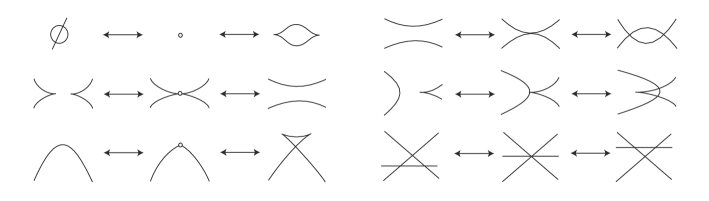
Figure 2. Apparent contour of germs with $\mathcal{A}_{e}$-codimension $1$ [16]: local singularity types are of lips, beaks, swallowtail (left), and multi-singularity types are of tacnode folds, cusp+fold, triple folds (right).

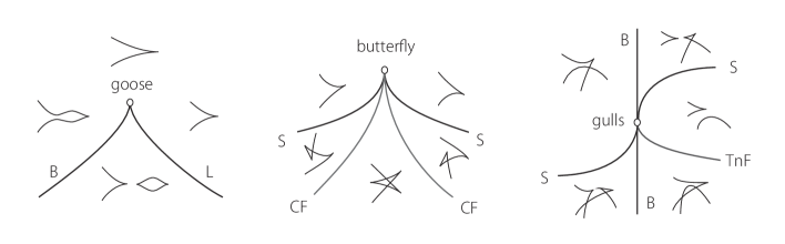
Figure 3. Bifurcation diagrams of singularities with corank one of $A_{e}$-codimension $2$: goose $(x,y^{3}+x^{3}y)$, butterfly $(x,xy+y^{5}+y^{7})$, gulls $(x,xy^{2}+y^{4}+y^{5})$.

3. Corank two singularities

3.1. Sharksfin and odd-shaped sharksfin

In Rieger-Ruas [23], $\mathcal{A}$-simple germs of corank $2$ have been classified. As seen before (Table 1), there are four types in codimension $\leq 3$, one of which is not $\mathcal{A}$-simple, that is the moduli of type $I_{2,3}$. The case of deltoid is easy: the bifurcation diagram consists only of the origin in the parameter plane, i.e., the singularity type has only adjacencies of fold and cusps, and no other local and multi-singularities; any small perturbation of this type produces a ‘deltoid-shaped’ apparent contour with three cusps (Fig.4, left). On the other hand, the bifurcation diagrams of sharksfin and odd-shaped sharksfin had been unclear for a long time [12, 28, 29].

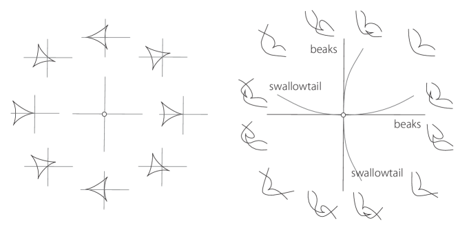
Figure 4. Bifurcation diagrams of singularities with corank two of $A_{e}$-codimension $2$: deltoid $(x^{2}-y^{2}+x^{3},xy)$ and sharksfin $(x^{2}+y^{3},y^{2}+x^{3})$ [9, 29]

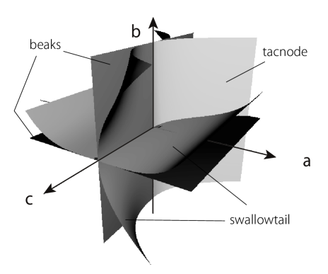
Figure 5. Bifurcation diagrams of odd-sharksfin [29]

3.1.1. Sharksfin

Let us consider the following miniversal unfolding of $I_{2,2}^{1,1}$:

(1) $$F(x,y,a,b)=(x^{2}+y^{3}+ay,y^{2}+x^{3}+bx).$$

In the parameter $ab$-plane, the bifurcation diagram $\mathcal{B}_{F}$ consists of four smooth curve-germs at the origin (for the swallowtail, it is computed up to degree $9$ in [28]):

Beaks:	$a=0$ and $b=0$
Swallowtail:	$a=\frac{1}{16}b^{4}+\frac{3}{32}b^{9}+o(9)$ and $b=\frac{1}{16}a^{4}+\frac{3}{32}a^{9}+o(9)$.

3.1.2. Odd-shaped sharksfin

Let us consider the following miniversal unfolding of $I_{2,2}^{2,1}$:

(2) $$F(x,y,a,b,c)=(x^{2}+y^{5}+cy^{3}+ay,y^{2}+x^{3}+bx).$$

The 3D picture of $\mathcal{B}_{F}$ is drawn in Fig.5. Although it is too hard to find an explicit form of the defining equation for the swallowtail stratum, we know how to draw it from the information about the bifurcation diagrams of types sharksfin and gulls.

Beaks:	$a=0$ and $b=0$
Swallowtail:	two smooth surfaces tangent to $ab=0$ along $c$-axis
	with $4$-point contact, one of which is tangent to $a=0$
	along the $b$-axis with $3$-point contact.
Tacnode:	$4a=c^{2}\;(c<0)$
Gulls:	$b$-axis

3.2. Bifurcation diagram of type $I_{2,3}$

It is known that the germ

$$I_{2,3}:(x,y)\mapsto(x^{2}+y^{3},xy)$$

is $\mathcal{A}$-finite, and is not $\mathcal{A}$-simple – it belongs to a moduli stratum of $\mathcal{A}$-orbits of the form $(x^{2}+y^{3}+\alpha xy^{2}+\beta y^{4}+\cdots,xy)$ with the modality $\geq 2$, see Rieger-Ruas [23]. Furthermore, as noted in Gaffney-Mond [8, Ex.5.11], any $\mathcal{A}$-finite germ contained in the $\mathcal{K}$-orbit is obtained by adding some higher terms to this germ, and hence the germ is topologically $\mathcal{A}$-equivalent to $I_{2,3}$ by a theorem of J. Damon, i.e., the $\mathcal{K}$-orbit has a unique topologically $\mathcal{A}$-type in its open dense subset. In other words, in the larger parameter space of an $\mathcal{A}_{e}$-miniversal unfolding of the $\mathcal{A}$-finite germ $I_{2,3}$, the bifurcation diagram is Whitney regular along the $\mathcal{A}$-moduli stratum. Therefore for our purpose, it suffices to take the following form of an unfolding of $\mathcal{A}$-type $I_{2,3}$ which corresponds to a normal slice to the stratum:

(3) $$G(x,y,a,b,c)=(x^{2}+y^{3}+ax+by+cy^{2},xy).$$

Namely, even if we add some terms $xy^{2},y^{4},\cdots$ to the first component, the unfolding remains to be transverse to the stratum in the space of all germs (or jets), and thus the bifurcation diagram is topologically the same by Thom’s isotopy lemma.

Note that $G$ is just a stable unfolding of $\mathcal{K}$-type of $I_{2,3}$: The structure of nearby $\mathcal{K}$-orbits was well investigated in Lander’s paper [14], in which the loci of swallowtail and butterfly of $\mathcal{B}_{G}$ are presented in an explicit form. Our first aim is to describe precisely all the strata of the bifurcation diagram $\mathcal{B}_{G}$ for local and multi $\mathcal{A}$-types.

Theorem 3.1.

Let $G$ be the topologically $\mathcal{A}_{e}$-versal unfolding (3) of $I_{2,3}$. Then the bifurcation diagram $\mathcal{B}_{G}$ consists of three components corresponding to types beaks-lips, swallowtail and cusp+fold, as drawn in Fig.7. Each stratum is explicitly parametrized as follows. For the complement to $\mathcal{B}_{G}$, apparent contours of corresponding stable maps are drawn in Fig.9.

Sharksfin	$c$-axis with $c>0$
Deltoid	$c$-axis with $c<0$
Beaks/Lips:	the surface with $A_{3}$-singularity at the origin whose
	double point curve is the locus of sharksfin; parametrized by
	$(a,b,c)=(\pm 4y\sqrt{c+3y},-y(4c+9y),c)$
Goose:	the cuspidal edge of the beaks/lips locus parametrized by
	$(\pm\frac{8}{9\sqrt{3}}c^{3/2},\frac{4}{9}c^{2},c)$ with $c>0$
Swallowtail:	the surface which contains the $a$-axis and the sharksfin locus;
	parametrized by
	$(a,b,c)=(\pm y(4c+15y)(c+4y)^{-1/2},-2y(2c+5y),c)$
Butterfly:	the cuspidal edge of the swallowtail locus parametrized by
	$(\pm\frac{1}{\sqrt{5}}c^{3/2},\frac{2}{5}c^{2},c)$ with $c>0$
Cusp+Fold:	the surface with $A_{3}$-singularity at the origin whose
	cuspidal edge is the butterfly locus; parametrized by
	$(a,b,c)=(\pm\sqrt{-y}(3c+5y),\frac{1}{4}(c^{2}-6cy-15y^{2}),c)\;\;(y<0)$

Remark 3.2.

It is remarkable that the odd-shaped sharksfin has the adjacency of gulls, but not butterfly and goose, while the type of $I_{2,3}$ has the adjacencies of butterfly and goose, but not gulls. That completes the adjacency diagrams among $\mathcal{A}$-orbits of $\mathcal{A}_{e}$-codimension $\leq 3$ as in Fig.6 (it corrects §3 of [23]). We follow the notation used in [20] for each $\mathcal{A}$-type.

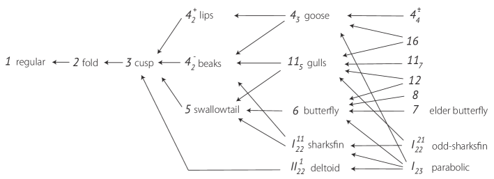
Figure 6. Adjacencies of local singularities up to $\mathcal{A}$-cod. $\leq 5$.

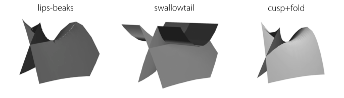
Figure 7. The bifurcation diagram in the parameter $3$-space consists of three ‘doggies’ components, beaks-lips locus (left), swallowtail locus (center), cusp+fold locus (right), and a ‘doggie’s tail’ component (one half of the $c$-axis with $c<0$) which is the deltoid locus. The picture of the swallowtail locus coincides with Fig.3 in Lander [14] (but from a different viewpoint).

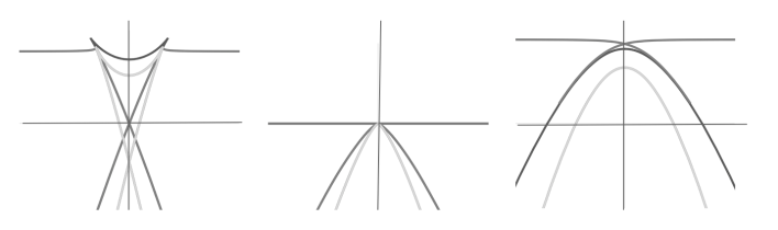
Figure 8. Sections of the bifurcation diagram with the plane $c=const.$ (positive, zero, negative, from left to right). The loci of beaks and swallowtail are very close to each other in a large part, where they are depicted to be overlapped. See Fig. 9.

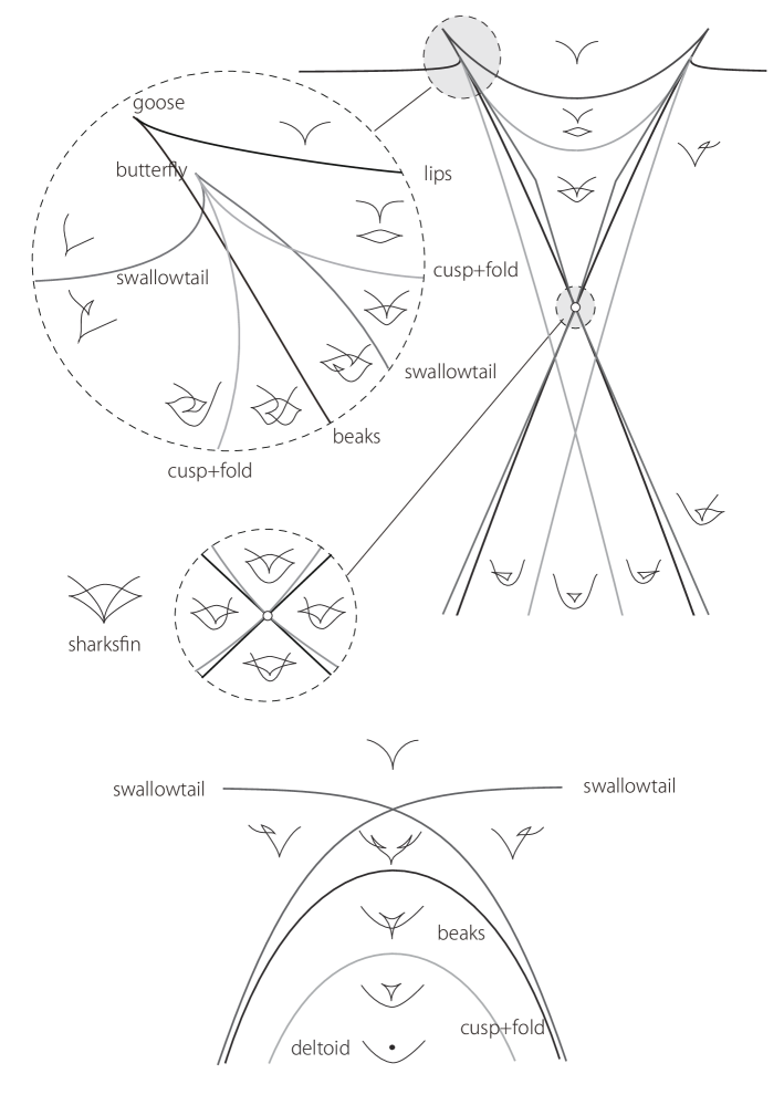
Figure 9. Bifurcation of apparent contours of map-germs corresponding to sections in Fig. 8 (left and right).

Proof :  To obtain above parameterizations we use the criteria in Table 2. For the unfolding given by (2), put

$$\textstyle\lambda=\left|\begin{array}[]{cc}\;2x+a&\;\;\;\;3y^{2}+2cy+b\\ \;y&\;\;\;\;x\end{array}\right|,$$

and take

$$\eta=-x\frac{\partial}{\partial x}+y\frac{\partial}{\partial y}$$

where $(x,y)\not=(0,0)$, otherwise $\eta=-(3y^{2}+2cy+b)\frac{\partial}{\partial x}+(2x+a)\frac{\partial}{\partial y}$.

To see the loci of sharksfin and deltoid is easy: $x=y=a=b=0\;(c\not=0)$. The sharksfin (resp. the deltoid) corresponds to $c>0$ (resp. $c<0$).

The beaks/lips locus is defined by

$$\textstyle\lambda=0,\;\frac{\partial}{\partial x}\lambda=a+4x=0,\;\frac{\partial}{\partial y}\lambda=-b-4cy-9y^{2}=0.$$

Solve $a,b$ in $x,y,c$ and substitute them into $\lambda=0$, then we have $x=\pm y\sqrt{c+3y}$ (thus in $xyc$-space it forms a crosscap $x^{2}=y^{2}(c+3y)$). This equality gives the above parametrization of $a=a(c,y)$ and $b=b(c,y)$. The picture of this locus is depicted in Fig.7 (left): It has a transverse self-intersection along the sharksfin locus. The defining equation is given by

$$243a^{4}+\left(256c^{3}-864bc\right)a^{2}+768b^{3}-256b^{2}c^{2}=0.$$

The strata of type lips and the beaks are separated by the goose curve: From the criteria (Table 2), we check $\mbox{H}_{\lambda}=0$ additionally; that implies $y=-\frac{2}{9}c\;(c>0)$, and hence the above parametrization is obtained. The goose curve is actually the cuspidal edge of the singular surface, which looks like the first doggies “ears”. The lips part is the “head”. The gulls type does not appear, since $\eta^{2}\lambda=0$ implies $x=y=a=b=0$.

The swallowtail locus is defined by

$$\lambda=\eta\lambda=\eta^{2}\lambda=0.$$

It is solved as follows. The computation is essentially the same as in Lander [14, §5.5], since $G$ is a stable unfolding of $\mathcal{K}$-type of $I_{2,3}$. By $\lambda=\eta\lambda=0$, we have

$$\textstyle a=\frac{1}{x}(-2x^{2}+by+2cy^{2}+3y^{3}),\;\;b=-\frac{1}{y}(x^{2}+3cy^{2}+6y^{3}),$$

unless $xy=0$, and then $\eta^{2}\lambda=0$ leads to $x=\pm y\sqrt{c+4y}$ (thus in $xyc$-space it forms a crosscap). This yields the above parameterization. Notice that the limit as $c,y\to 0$ is the $a$-axis; In fact, if $x=0$ or $y=0$, three equations imply $x=y=b=c=0$, hence the $a$-axis belongs to this locus. The defining equation of the locus is

$$80a^{4}\left(8b-3c^{2}\right)-8a^{2}\left(285b^{2}c-192bc^{3}+32c^{5}\right)+b^{2}\left(45b-16c^{2}\right)^{2}=0,$$

and the picture is Fig.7 (center). It has a transverse self-intersection along the sharksfin locus: The beaks and the swallowtail loci have $4$-point contact along this half line, that is verified by the bifurcation diagram of the sharksfin. For the butterfly, we add one more equation $\eta^{3}\lambda=-24y^{3}(c+5y)=0$, that implies $y=-c/5\;(c>0)$; The butterfly curve also looks “ears” of the second doggie, i.e., it is the cuspidal edge of the locus of swallowtail.

The locus of cusp + fold (bi-germ) must appear, since it is adjacent to the butterfly. The equations are:

$$xy=XY,\;ax+x^{2}+by+cy^{2}+y^{3}=aX+X^{2}+bY+cY^{2}+Y^{3},$$

$$\lambda(x,y)=\lambda(X,Y)=0,\;\eta\lambda(x,y)=0.$$

We can eliminate $a,b$ by the third and fourth equations $\lambda=0$; then the second equation gives $X=\pm y\sqrt{c+2(y+Y)}$, and hence the last equation eliminates $x$, then $Y=-\frac{1}{2}(c+3y)$. Thus we can express $a,b,x$ using variables $c,y$. The parametrization leads to Fig.7 (left). This third doggie also has “ears” along the butterfly curve, as same as the second one does. The defining equation is

$$18225a^{8}+14580a^{6}c^{3}-54a^{4}\left(1275b^{2}c^{2}-49c^{6}\right)$$

$$+108a^{2}\left(500b^{4}c-15b^{2}c^{5}-c^{9}\right)-\left(16b^{2}-c^{4}\right)\left(c^{4}-25b^{2}\right)^{2}=0.$$

In a similar way as seen above, direct computations show that no other multi-singularity strata appear. $\Box$

4. Parallel projection of parabolic crosscaps

4.1. Projection of smooth surface in $3$-space

We begin with projecting a smooth surface to the plane. Let $M$ be a fixed smooth surface in $\mathbb{R}^{3}$, and $\Pi_{\ell}:\mathbb{R}^{3}\to\mathbb{R}^{2}$ a linear projection with the kernel line $\ell\subset\mathbb{R}^{3}$, then the restriction $\Pi_{\ell}|_{M}:M\to\mathbb{R}^{2}$ is called a parallel projection of $M$ along the direction $\ell$. When $\ell$ varies, it defines locally a family of plane-to-plane maps with two parameters; V. I. Arnold [1, 2] and W. Bruce [4] classified singularities of the parallel projection for an appropriately generic surface up to the $\mathcal{A}$-equivalence defined by local diffeomorphisms of $M$ and the target $\mathbb{R}^{2}$ (the screen). Such a generic surface is stratified according to the local singularity types of the projection. In particular, there are two major characteristic curves on $M$:

• The parabolic curve consists of points where the Gaussian curvature vanishes; At each point there is only one asymptotic line, and the parallel projection along the asymptotic line admits the lips and the beaks or more degenerate singularity.

• The flecnodal curve consists of points where an asymptotic line has at least $4$-point contact with the surface; or equivalently, points where the Pick invariant vanishes; the parallel projection along the asymptotic line has the swallowtail or more degenerate singularity.

Note that these two curves meet tangentially at some isolated points, called the godrons, where the projection admits the gulls singularity.

Furthermore, not fixing a generic surface, we may consider a generic $1$-parameter family of embeddings $\iota_{t}:M\hookrightarrow\mathbb{R}^{3}$ ($t\in I$, where $I$ is an open interval); In relation with an application to Computer Vision, J. Rieger [22] studied singularities arising in the family $\Pi_{\ell}\circ\iota_{t}$ with three parameters $\ell$ and $t$, and showed that all singularity types of $\mathcal{A}_{e}$-codimension $\leq 3$ arise generically.

Remark 4.1.

In relation with projective geometry of surfaces, singularities in the central projection from arbitrary viewpoint has been studied by Arnold et al [1, 2, 19, 10]. For central projections of a moving surface, see Kabata [13]. The classification of singularities for central projections becomes slightly different from that for parallel projections. For instance, the goose singularity appears in parallel projection at some isolated parabolic points in a generic surface, while the singularity type always arises in central projection at any parabolic point, when viewing it from some special viewpoint lying on the asymptotic line (Note that the parallel projection corresponds to the central projection with the viewpoint at infinity). In this paper we only consider the parallel projection.

4.2. Projection of crosscaps in $3$-space

As a generalization, J. West [25] considered singularities of parallel projection $\Pi_{\ell}\circ\iota:M\to\mathbb{R}^{2}$ where $\iota:M\to\mathbb{R}^{3}$ is a smooth map having crosscaps. That is the (unique) locally stable singularity type, and if one take suitable local coordinates of source and target, the map-germ is written by $(y,xy,x^{2})$. Since we are discussing the affine or flat geometry of the singular surface in $\mathbb{R}^{3}$, the ambient coordinate changes should be only affine transformation of $\mathbb{R}^{3}$, then the affine normal form is given by

(4) $$\iota(x,y)=(y,xy+g(x),x^{2}+\alpha y^{2}+\phi(x,y))$$

for a constant $\alpha$, $g(x)=d_{4}x^{4}+h.o.t.$ and $\phi(x,y)=c_{03}y^{3}+c_{12}xy^{2}+\cdots$ ([25]). We call it an elliptic, hyperbolic and parabolic crosscap, when $\alpha>0$, $\alpha<0$, $\alpha=0$, respectively. Obviously, when projecting the crosscap along its image tangent line $\ell=d\iota(TM_{x_{0}})$, the germ of $\Pi_{\ell}\circ\iota$ at $x_{0}$ is of corank $2$.

Theorem 4.2.

(Parabolic curve [25, Chap.5]) The parabolic curve does not approach to any hyperbolic crosscap, while there are two smooth branches of parabolic curve approaching to any elliptic crosscap. For generic $\iota:M\to\mathbb{R}^{3}$ in the space of all maps having crosscaps, the singular germ $\Pi_{\ell}\circ\iota$ of corank $2$ is $\mathcal{A}$-equivalent to either the sharksfin or the deltoid in Table 1 (then we call it a generic elliptic or hyperbolic crosscap).

On the other hand, it seems that the flecnodal curve on the singular surface with crosscap had not been taken attention. In our previous paper, we showed that

Theorem 4.3.

(Flecnodal curve [29, Thm. 1.3, 1.4]) The flecnodal curve does not approach to any hyperbolic crosscap, while there are two smooth branches of flecnodal curve approaching to any elliptic crosscap. Assume that $\iota$ has an elliptic crosscap at $x_{0}\in M$. Then, in the source space, each branch of the flecnodal curve is tangent to a branch of the parabolic curve with odd contact order at $x_{0}$; In particular, both pairs of branches have $3$-point contact if and only if the singular projection $\Pi_{\ell}\circ\iota$ is of type sharksfin (i.e, it is a generic elliptic crosscap).

Now let us discuss a singular version of Rieger’s observation on the projection of a moving surface [21]; Parallel projections of one-parameter families of crosscaps should be related to corank two map-germs of $\mathcal{A}_{e}$-codimension $3$. We obtain the following theorem:

Theorem 4.4.

(Projection of non-generic crosscap) For a generic one-parameter family $M\times I\to\mathbb{R}^{3}$, $(x,t)\mapsto\iota_{t}(x)$ of smooth maps having crosscaps (for all $t$), the germ of parallel projection $\Pi_{\ell}\circ\iota_{0}:M\to\mathbb{R}^{3}$ admits the odd-shaped sharksfin and the type of $I_{2,3}$. The bifurcation of parabolic/flecnodal curves on the singular surface with respect to the parameter $t$ are described in Fig.10 and Fig.11.

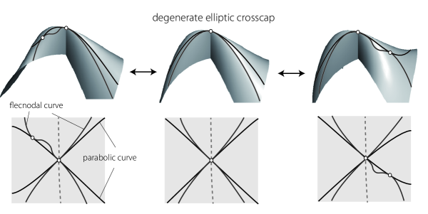
Figure 10. Bifurcation of degenerate elliptic crosscap [29]. The upper pictures depict the bifurcation of the parabolic/flecnodal curves on the singular surface in $3$-space, while the lower pictures depict the corresponding loci in the source space of the parametrization (the dotted curve is the double point locus in the source). In the source, the degenerate crosscap (center) has a pair of branches of parabolic/flecnodal curves with $5$-point contact. It is deformed into a generic elliptic crosscap (where two curves has $3$-point contact) and a godron ($2$-point contact).

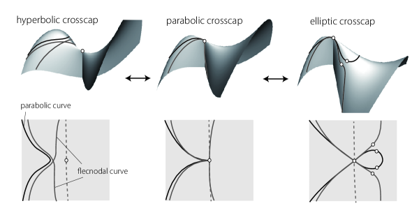
Figure 11. Bifurcation of parabolic crosscap. The bifurcation of the parabolic curve in source is given by a $1$-parameter family of sections of a crosscap (cf. Nuño-Ballesteros-Tari [15]). The flecnodal curve locally consists of two irreducible analytic branches. Deforming the parabolic crosscap, there appear a generic elliptic crosscap, two points of type goose, and two points of type butterfly, otherwise a hyperbolic crosscap and a double point of the flecnodal curve. The corresponding bifurcation diagram in the parameter space of view-lines $\ell$ is the same as Fig.8.

Proof :  In [29] the assertion has been proved for the case of odd-shaped sharksfin, i.e., projecting the least non-generic elliptic crosscaps in the sense mentioned above. Here we deal with the case of $I_{2,3}$, i.e., projecting parabolic crosscaps.

Suppose that we are given a smooth map $\iota:M\to\mathbb{R}^{3}$ with a parabolic crosscap at $x_{0}=(0,0)$. A generic $1$-parameter deformation $\iota_{t}:M\to\mathbb{R}^{3}$ of $\iota_{0}=\iota$ ($t$ sufficiently small) may be written as

(5) $$\iota_{t}(x,y)=\left(y,xy+g(x,y,t),x^{2}+ty^{2}+\phi(x,y,t)\right),$$

where for each $t$ fixed, $j^{2}g(0)=0$, $j^{2}\phi(0)=0$ and $g(x,y,0)$ does not depend on $y$, via source coordinate changes and an affine transformation of target $\mathbb{R}^{3}$ depending on $t$ (cf. [17, Prop. 4.1], [15]). The image tangent line at the parabolic crosscap is generated by $(1,0,0)$, and we put $U=\mathbb{R}^{2}$ of lines $\ell$ generated by $(1,v,w)$. The parallel projection of the singular surface $\iota_{t}(M)$ along $\ell$ defines a family of smooth maps $\varphi:M\times U\times\mathbb{R}\to\mathbb{R}^{2}$ by

$$\varphi(x,y,v,w,t)=\left(xy-vy+g(x,y,t),x^{2}+ty^{2}-wy+\phi(x,y,t)\right).$$

For general choices of $g,\phi$ such as $\phi=c_{03}y^{3}+\cdots\;(c_{03}\not=0)$ etc, the plane-to-plane germ $\varphi(x,y,0,0,0)$ is $\mathcal{K}$-equivalent to $I_{2,3}$ and $\varphi(x,y,v,w,t)$ is a stable unfolding of this singularity type. Hence, generically, $\varphi$ can be regarded as a topologically versal unfolding of some germ belonging to the $\mathcal{A}$-moduli stratum of type $I_{2,3}$ (cf. Gaffney-Mond [8]). Thus the bifurcation diagram of $\varphi$ is obtained by a slightly modified $\mathcal{B}_{G}$ in Fig.7 – in particular, $\varphi(x,y,v,w,0)$ corresponds to a generic $2$-dimensional section of $\mathcal{B}_{G}$ through the origin, like as in Fig.12, and is homeomorphic to the middle of Fig.8. As $t$ varies from $0$, the section bifurcates in a similar way as depicted in Fig.8 (right and left).

We have just seen the bifurcation of singular view-direction parameters $(u,v)$ with respect to $t$, and now let us turn to see bifurcations of the parabolic curve and the flecnodal curve on the singular surface. Since we are interested in the topological type, we take at first a typical one of the form (5)

$$\iota_{t}(x,y)=\left(y,xy,x^{2}+ty^{2}+y^{3}\right)$$

i.e., $g=0$, $\phi=y^{3}$. The parallel projection $\varphi$ described above is equivalent to $G$ in (3) via the coordinate changes $(\bar{x},\bar{y})=(x-v,y)$ of the source and $(\bar{X},\bar{Y})=(X,Y-v^{2})$ of the target together with $(a,b,c)=(2v,-w,t)$ of parameters. As shown in the proof of Theorem 3.1, the beaks-lips curve is given by $\bar{x}^{2}=\bar{y}^{2}(c+3\bar{y})$ and $a=-4\bar{x}$, and the swallowtail curve is given by $\bar{x}^{2}=\bar{y}^{2}(c+4\bar{y})$ and $a=\pm\bar{y}(4c+15\bar{y})(c+4\bar{y})^{-1/2}$. Hence substituting $(\bar{x},\bar{y})=(x-a/2,y)$ to these equations, parabolic and flecnodal curves are obtained, respectively, such as

$$\textstyle x^{2}=y^{2}(t+3y),\quad x^{2}(t+4y)=y^{2}(t+\frac{7}{2}y)^{2}.$$

When $t=0$, the parabolic curve has an ordinary cusp at the origin, while the flecnodal curve consists of two irreducible components, an ordinary cusp and a line $y=0$. The line is also the double point curve in this special from, but it is not the case in general: it can be seen that the component is tangent to the double-point curve at the origin. In fact, for general choices of $g,\phi$, above two equations are modified by adding functions of order $\geq 3$ (with respect to $x,y$), hence the local pictures around the origin do not change topologically, as depicted in Fig.11. $\Box$

Figure 12. A generic plane section of $\mathcal{B}_{G}$ though the origin.

Remark 4.5.

(Goose and butterfly) In Fig.11, for $t>0$, the parabolic curve (black) has two parts corresponding to the beaks and the lips types of projection along the asymptotic line, which are separated by two points of goose type; the flecnodal curve (gray) has two points of type butterfly at which an asymptotic line has $5$-point contact with the surface. For $t<0$, the parabolic curve consists of a smooth component and an isolated point which is a hyperbolic crosscap, and the flecnodal curve consists of two smooth components meeting each other at a point transversely where both of two asymptotic lines have $5$-point contact with the surface.

Remark 4.6.

(Foliation of asymptotic curves) An asymptotic curve on a smooth surface in $\mathbb{R}^{3}$ is by definition the integral curve of the field of asymptotic lines, which is described as the solution of a binary differential equation (Bruce-Tari [5]). All such curves form a pair of foliations on the hyperbolic domain and have cusp singularities at the parabolic points of the surface. The flecnodal curve is just the curve of inflection points of asymptotic curves. Near a crosscap point, the configuration of the asymptotic curves has been studied in Tari [26] (for elliptic and hyperbolic crosscaps) and Oliver [17] (for parabolic crosscaps) – for instance, look at pictures of these foliations, Fig.1 and Fig.9 in [17], then we may experimentally trace the curve of inflection points of asymptotic curves, that would convince us of our pictures Fig.10 and Fig.11 above. We will discuss somewhere in detail about these two different approaches using BDE and parallel projection.

5. Appendix: Planar caustics of parabolic umbilic type

We briefly discuss an application to the planar parabolic umbilic caustics (Thom [27]). First we explain a few definitions. Let us consider the $\mathcal{R}^{+}$-miniversal deformation of the $D_{5}$ singularity of function-germ

$$F(x,y,\mu_{1},\mu_{2},q_{1},q_{2}):=x^{2}y+\frac{1}{4}y^{4}+\frac{q_{2}}{3}y^{3}+\frac{q_{1}}{2}y^{2}-2\mu_{1}x-\mu_{2}y$$

(usually one uses $x^{2}$ instead of the term of $y^{3}$). The catastrophe set $C$ in $\mathbb{R}^{6}=\mathbb{R}^{2}\times\mathbb{R}^{4}$ is defined by $\frac{\partial F}{\partial x}=\frac{\partial F}{\partial y}=0$, hence $C$ is parametrized by $x,y,q_{1},q_{2}$ so that

(6) $$\mu_{1}=xy,\quad\mu_{2}=x^{2}+y^{3}+q_{1}y+q_{2}y^{2}.$$

The corresponding Lagrange map $\Phi:C,0\to\mathbb{R}^{4},0$ is just the projection of $C$ to the parameter space, $(x,y,q_{1},q_{2})\mapsto(\mu_{1},\mu_{2},q_{1},q_{2})$.

We are interested in generic $2$-dimensional sections of the big-caustics (the critical value set of $\Phi$) in $4$-space, see [29, §4.1] for a precise formulation. Let $\rho:\mathbb{R}^{4},0\to\mathbb{R}^{2},0$ be a submersion so that $\Phi$ is transverse to the smooth level set $\rho^{-1}(0)$ at the origin. Note that if we put $S_{t}=\rho^{-1}(t)$ for each $t=(t_{1},t_{2})\in\mathbb{R}^{2}$ small enough, the condition says that $\Phi^{-1}(S_{t})$ is smooth and the restrictions $\Phi:\Phi^{-1}(S_{t})\to S_{t}$ form a $2$-parameter family of Lagrange maps. We now describe the family of Lagrange maps simply as a family of plane-to-plane maps (that corresponds to the so-called caustics-equivalence). Since $\Phi$ has corank $2$ and $\rho\circ\Phi$ is submersive, we may assume that $\rho$ is of the form

$$t_{1}=q_{1}-a_{1}\mu_{1}-a_{2}\mu_{2}+O(2),\quad t_{2}=q_{2}-b_{1}\mu_{1}-b_{2}\mu_{2}+O(2).$$

Solve $q_{1},q_{2}$ in terms of $\mu_{1},\mu_{2},t_{1},t_{2}$, and substitute them into (6), then by further coordinate changes of $(x,y)$ depending on $t_{1},t_{2}$, we see that $\Phi$ is $\mathcal{A}$-equivalent to $\Xi:(x,y,t_{1},t_{2})\mapsto(\mu_{1},\mu_{2},t_{1},t_{2})$ with

$$\mu_{1}=xy,\quad\mu_{2}=x^{2}+y^{3}+a_{1}xy^{2}+t_{1}y+t_{2}y^{2}+\phi,$$

where $j^{3}\phi(x,y,0,0)=0$ and $\frac{\partial\phi}{\partial t_{i}}(x,y,0,0)=0$. For general $\rho$, we may think of $\Xi$ as an unfolding of the germ belonging to the $\mathcal{A}$-moduli of type $I_{2,3}$; Then the bifurcation diagram $\mathcal{B}_{\Xi}$ is obtained at least topologically as a small perturbation of the $bc$-plane section of $\mathcal{B}_{G}$ with fixing the $c$-axis, where $G$ is the normal form of (3), see Fig.13. Thus the topological type is unique as depicted in Fig.14.

Figure 13. Typical section of $\mathcal{B}_{G}$ with fixing the $c$-axis.

In $\mathbb{R}^{4}$ the big-caustics are only of type $A_{\mu}\;(\mu\leq 5)$, $D_{4}$ and $D_{5}$. Each $\mathcal{A}$-type of corank one plane-to-plane germs can be realized by planar Lagrange map-germs, and hence generic multi-parameter bifurcations of planar caustics of type $A_{\mu}$ are the same as bifurcation diagrams of corank one germs. In [29], we have studied some topological types of bifurcatoins of planar $D_{4}$-caustics, and generic $2$-paramter bifurcation of type $D_{5}$ has been discussed above. Those lead a fairly natural extension of the perestroikas (=generic $1$-parameter bifurcations) of planar caustics due to Arnold-Zakalyukin [1].

As an additional remark, each $\mathcal{A}$-type of corank two plane-to-plane germs can be realized by projecting singular Lagrange surface with open Whitney umbrella, see Bogaevski-Ishikawa [3].

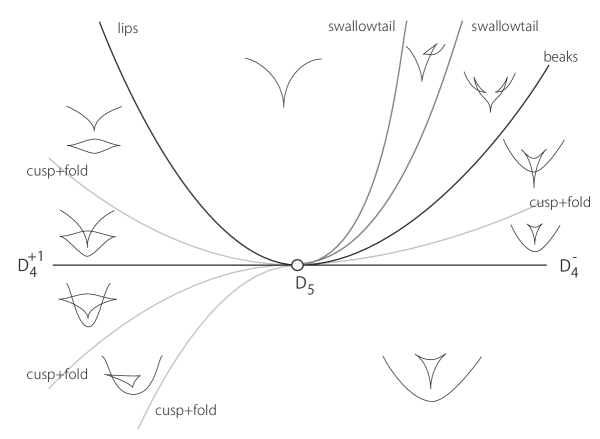
Figure 14. Generic bifurcation of planar caustics of type $D_{5}$.

References

- [1] V. I. Arnold, Catastrophe Theory, 3rd edition, Springer (2004).
- [2] V. I. Arnold, V. V. Goryunov, O. V. Lyashko, V. A. Vasil’ev, Singularity Theory II, Classification and Applications, Encyclopaedia of Mathematical Sciences Vol. 39, Dynamical System VIII (V. I. Arnold (ed.)), (translation from Russian version), Springer-Verlag (1993).
- [3] I. A. Bogaevski and G. Ishikawa, Lagrange mappings of the first open Whitney umbrella, Pacific Jour. Math. 203 (1) (2002), 115–138.
- [4] J. W. Bruce, Projections and reflections of generic surfaces in , Math. Scand. 54 (1984), 262–278.
- [5] J. W. Bruce and F. Tari, On binary differential equations, Nonlinearity 8 (1995), 255–271.
- [6] J. W. Bruce and J. West, Functions on a cross-cap, Math. Proc. Phil. Soc. 123 (1998), 19–39.
- [7] T. Fukui and M. Hasegawa, Singularities of parallel surfaces, Tohoku Math. J. 64 (2012), 387-408.
- [8] T. Gaffney and D. Mond, Weighted homogeneous maps from the plane to the plane, Math. Proc. Cambridge Phil. Soc. 109 (1991), 451–470.
- [9] C. G. Gibson and C. A. Hobbs, Singularity and Bifurcation for General Two Dimensional Planar Motions, New Zealand J. Math. 25 (1996) 141–163.
- [10] V.V. Goryunov, Singularities of projections of complete intersections, J. Soviet Math. 27 (1984), 2785–2811 [Translated from Itogi Nauki i Tekhniki. Ser. Sovrem. Probl. Mat. 22 (1983),167–206.]
- [11] M. Hasegawa, A. Honda, K. Naokawa, M. Umehara and K. Yamada, Intrinsic invariants of cross caps, preprint, arXiv:1207.3853 (2012).
- [12] W. Hawes, Multi-dimensional Motions of the Plane and Space, Dissertation, University of Liverpool (1994).
- [13] Y. Kabata, Recognition of plane-to-plane map-germs, preprint (2015), arXiv:1503.08544.
- [14] L. Lander, The structure of the Thom-Boardman singularities of stable germs with type , Proc. London Math. Soc. 33 (1976), 113–137.
- [15] J. Nuño-Ballesteros and F. Tari, Surface in and their projections to -spaces, Proc. Royal Soc. Edinburgh Sect. A 137 (2007), 1313–1328.
- [16] T. Ohmoto and F. Aicardi, First order local invariants of apparent contours, Topology, 45 (2006) 27-45.
- [17] J. M. Oliver, On pairs of foliations of a parabolic cross-cap, Qual. Theory Dyn. Syst.10 (2011), 139–166.
- [18] R. Oset-Sinha and F. Tari, Projections of surfaces in to and geometry of their singular images, Rev. Math. Iberoam. European Math. Soc. 31 (2015), 33–50, DOI: 10.4171/RMI/825.
- [19] O. A. Platonova, Projections of smooth surfaces, J. Soviet Math. 35 (1986), 2796–2808 [Tr. Sem. I. G. Petrovskii 10 (1984), 135–149 in Russian].
- [20] J. H. Rieger, Families of maps from the plane to the plane, J. London Math. Soc. (2) 36 (1987), no. 2, 351-369.
- [21] J. H. Rieger, Versal topological stratification and the bifurcation geometry of map-germs of the plane, Math. Proc. Cambridge Philos. Soc.107 (1990), 127-147.
- [22] J. H. Rieger, The geometry of view space of opaque objects bounded by smooth surfaces, Artificial Intelligence, 44 (1990), 1-40.
- [23] J. H. Rieger and M. A. S. Ruas, Classification of -simple germs from to , Compositio Math. 79 (1991), 99-108.
- [24] K. Saji, Criteria for singularities of smooth maps from the plane into the plane and their applications, Hiroshima Math. Jour. 40 (2010), 229–239.
- [25] J. West, The Differential Geometry of the Cross-Cap, Dissertation, University of Liverpool (1995).
- [26] F. Tari, Pairs of geometric foliations on a crosscap, Tohoku Math. J., 59 (2007), 226–233.
- [27] Thom, R., Structural Stability and Morphogenesis, W. A. Benjam, (1972).
- [28] T. Yoshida, Bifurcation of plane-to-plane map-germs of corank and application to robotics (in Japanese), Master thesis, Hokkaido University (2014).
- [29] T. Yoshida, Y. Kabata and T. Ohmoto, Bifurcation of plane-to-plane map-germs of corank , Quarterly Jour. Math. (2014) doi:10.1093/qmath/hau013