Transport through an Anderson impurity: Current ringing, non-linear magnetization and a direct comparison of continuous-time quantum Monte Carlo and hierarchical quantum master equations

Abstract

We give a detailed comparison of the hierarchical quantum master equation (HQME) method to a continuous-time quantum Monte Carlo (CT-QMC) approach, assessing the usability of these numerically exact schemes as impurity solvers in practical nonequilibrium calculations. We review the main characteristics of the methods and discuss the scaling of the associated numerical effort. We substantiate our discussion with explicit numerical results for the nonequilibrium transport properties of a single-site Anderson impurity. The numerical effort of the HQME scheme scales linearly with the simulation time but increases (at worst exponentially) with decreasing temperature. In contrast, CT-QMC is less restricted by temperature at short times, but in general the cost of going to longer times is also exponential. After establishing the numerical exactness of the HQME scheme, we use it to elucidate the influence of different ways to induce transport through the impurity on the initial dynamics, discuss the phenomenon of coherent current oscillations, known as current ringing, and explain the non-monotonic temperature dependence of the steady-state magnetization as a result of competing broadening effects. We also elucidate the pronounced non-linear magnetization dynamics, which appears on intermediate time scales in the presence of an asymmetric coupling to the electrodes.

I Introduction

Impurity problems are ubiquitous in the theoretical description of nonequilibrium systems Andergassen et al. (2010); Aoki et al. (2014). They constitute small entities with a limited number of degrees of freedom that are coupled to reservoirs with continua of non-interacting degrees of freedom. One intuitive physical realization of such a model is a molecule adsorbed on a surface or contacted by electrodes Cuevas and Scheer (2010). A variety of nonequilibrium scenarios may be described in terms of impurity models, for instance by preparing the impurity in an excited initial state or by coupling it to different reservoirs in different thermodynamic states. Another intriguing application occurs in dynamical mean field theory Georges et al. (1996); Freericks et al. (2006); Vollhardt (2012); Aoki et al. (2014), where lattice problems either in or out of equilibrium are mapped to impurity problems with an environment that is determined by a self-consistency criterion. This has been important, for instance, in understanding the metal–insulator transition in materials like transition metal oxides Georges et al. (1996); Nekrasov et al. (2005); Vollhardt (2012) and has become an important paradigm in studying nonequilibrium effects in extended interacting systems, including thermalization after an interaction quench Eckstein et al. (2009); Tsuji et al. (2013), the nonequilibrium steady state Joura et al. (2008); Aron et al. (2013) and Bloch oscillations Freericks et al. (2006); Freericks (2008); Eckstein and Werner (2011) under the influence of a static electric field. Thus, the theoretical description of impurity problems is a key element in understanding a wide range of phenomena, in particular nonequilibrium effects.

Few exact solutions are available, and a number of methods have been developed in the past decades to solve nonequilibrium impurity problems. They can be sorted into two broad categories: approximate and numerically exact methods. Typically, numerically exact methods allow us to simulate some property of a model in what might be considered a numerical experiment. Approximate methods, on the other hand, may miss important physics or suffer from artifacts due to the approximations involved. A combination of methods, which operate on different levels of approximation is often useful and helps to elucidate the relevant physical mechanisms Wang et al. (2008); Eckel et al. (2010); Werner et al. (2010); Schmitt and Anders (2010); Wang et al. (2011); Härtle et al. (2013); Härtle and Millis (2014).

The nonequilibrium Anderson impurity model has been treated by several numerically exact methodologies. Some approaches require a discretization of the electrodes, for example density-matrix renormalization group Al-Hassanieh et al. (2006); Dias da Silva et al. (2008); Kirino et al. (2008); Heidrich-Meisner et al. (2009); Kirino et al. (2010); Branschädel et al. (2010), numerical renormalization group Anders (2008a, b); Schmitt and Anders (2010) or multilayer multiconfiguration time-dependent Hartree theory Wang and Thoss (2013); Balzer et al. (2015). These methods are useful at low temperatures and/or voltages. They are restricted by revival oscillations and a limited spectral resolution of the leads Žitko and Pruschke (2009). Other approaches can take advantage of the noninteracting nature of the leads and do not require discretization. This includes iterative path-integral schemes Weiss et al. (2008); Segal et al. (2010, 2011); Hützen et al. (2012); Weiss et al. (2013), which converge only for a limited set of parameters, and stochastic schemes Werner et al. (2006); Schmidt et al. (2008); Werner et al. (2009); Schiró (2010); Gull et al. (2011a); Mühlbacher et al. (2011); Cohen et al. (2013a), where the growth of the statistical error restricts the accessible time scales. In the presence of a short memory timescale, long time scales can be accessed by a combination of reduced dynamics techniques Cohen and Rabani (2011) with a short-time numerically exact scheme; or by the hierarchical master equation method Zheng et al. (2009) where the numerical effort scales linearly with the simulation time. The latter, however, can only be converged if the temperature in the electrodes is not too low Härtle et al. (2013); Härtle and Millis (2014).

The numerical effort associated with most numerically exact schemes restricts practical calculations to specific limits Paaske and Flensberg (2005) or limited ranges of parameters. It is important to delineate the regimes in parameter space to which each method is applicable, and in particular to find out where exact results are not available. In this work, we elucidate the practical limitations of two numerically exact schemes: the continuous-time quantum Monte Carlo (CT-QMC) method Werner et al. (2006); Mühlbacher and Rabani (2008); Werner et al. (2009); Schmidt and Komnik (2009); Schiró and Fabrizio (2009); Gull et al. (2011a); Cohen and Rabani (2011); Cohen et al. (2013a) and the hierarchical quantum master equation (HQME) method Tanimura (2006); Welack et al. (2006); Jin et al. (2008); Härtle et al. (2013); Härtle and Millis (2014). We will discuss the main features of these approaches, characterizing, in particular, the associated numerical effort. We find that the range of parameters where the two methods can be applied overlaps, but also exhibits areas where only one of the methods can be applied. As we will see, HQME turns out to be the method of choice to study long-term dynamics if the temperature of the reservoirs is not too low. In contrast, CT-QMC gives access to the short- and intermediate-time dynamics over a wider range of temperatures.

We demonstrate our findings using an archetypal nonequilibrium problem: transport through a single-site Anderson impurity that is coupled to left and right electrodes (see Fig. 1 for a graphical representation). The most obvious physical realizations of this impurity problem are quantum dots containing a single spin-degenerate level. The first such realizations were based on quantum-confinements in patterned semiconductor heterostructures Cronenwett et al. (1998); Goldhaber-Gordon et al. (1998). Single-molecule junctions often exhibit similar behavior Liang et al. (2002); Pasupathy et al. (2004); Osorio et al. (2007); Roch et al. (2008), but in a setting where experimental techniques give less control over the parameters of the junction. Additionally, other effects, e.g. due to vibrational degrees of freedom, are important Yu et al. (2004); Sapmaz et al. (2005); Pasupathy et al. (2005); Thijssen et al. (2006); Parks et al. (2007); Böhler et al. (2007); de Leon et al. (2008); Repp et al. (2010); Ballmann et al. (2010, 2012, 2013). In these systems, transport is induced by shifting the electrochemical potentials in the leads with respect to each other such that electrons tunnel through the impurity in order to move from the lead with higher chemical potential to that with lower chemical potential. In semiconductor heterostructures this shift is achieved by charging or discharging the leads (i.e. by filling or emptying electronic levels; cf. Fig. 1b). In single-molecule junctions, the leads are less likely to be charged, and the shift of the electrochemical potentials is accompanied by a shift of the respective conduction bands (cf. Fig. 1c). We will show that these different ways of inducing transport strongly affect the initial dynamics of the impurity.

We also present exact results for the complex magnetization dynamics of an Anderson impurity in various nonequilibrium situations. Typically, this quantity exhibits the slowest relaxation behavior Cohen et al. (2013a) and, as we will see, exhibits a non-linear behavior on all times scales, in particular when an asymmetric coupling to the electrodes is considered. To date, this dynamics had only been accessible at great computational cost using state-to-the-art CT-QMC methods combined with reduced dynamics Cohen et al. (2013a). The HQME method gives access to exact results of this long-lived correlated dynamics and allows us to perfrom a scan over a wide range of parameters. It can also be used to derive approximate results and, therefore, to study the influence of higher order processes. We are, therefore, able to elucidate the origin of the non-monotonic temperature dependence of the magnetization that was recently reported in Ref. Cohen et al. (2013a) to be the result of competing broadening effects. We also find a pronounced non-linear behavior of the magnetization on intermediate (still rather long) time scales (cf.  e.g., Figs. 7 and 9). In passing we note that the nonequilibrium Anderson impurity model and its generalizations are of great interest in the field of strongly correlated materials within the dynamical mean field theory approximation Georges et al. (1996); Freericks et al. (2006); Vollhardt (2012); Aoki et al. (2014).

(a)	(b)		(c)

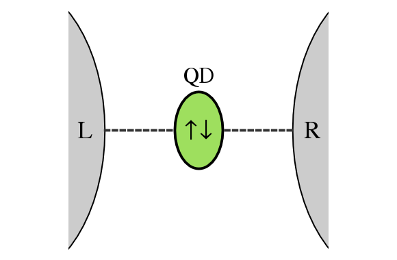
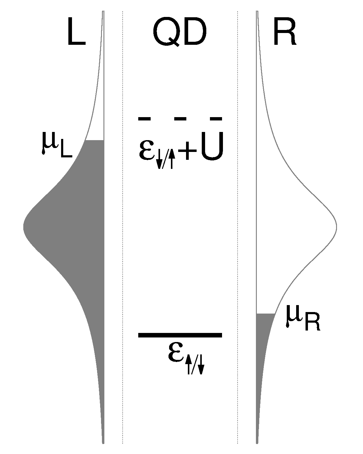
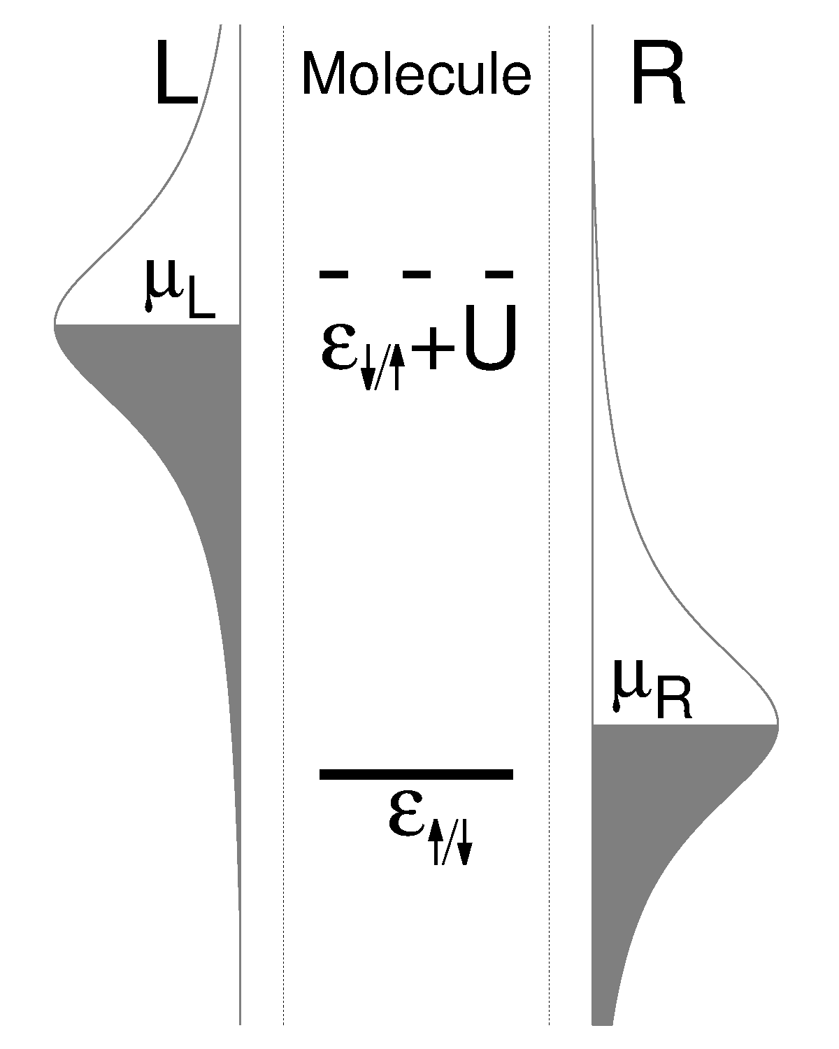
Figure 1: Panel (a): Graphical representation of an Anderson impurity, which is realized by a quantum dot (QD). The dot is coupled to a left (L) and a right electrode (R). Panel (b): Single-particle levels of the quantum dot junction depicted in Panel (a). The shaded areas depict the occupied states in the electrodes, which, for simplicity, are assumed to provide Lorentzian-shaped conduction bands. Applying a bias voltage to such a system means that the corresponding chemical potentials $\mu_{\text{L/R}}$ are shifted and the electrodes become charged. Panel (c): Single-particle levels of a molecular junction. In contrast to the quantum dot realization (Panels (a) and (b)), the conduction bands are shifted in the same way as the chemical potentials. Thus, applying a bias voltage, the electrodes do not become charged.

The outline of the article is as follows: In Sec. II, we present the theoretical methodology. This includes a short description of the single-site Anderson impurity model (Sec. II.1), the HQME method (Sec. II.2) and the CT-QMC approach (Sec. II.3). A discussion of practical aspects of the two methods is given in Sec. II.4. Numerical results on the time-dependent transport properties of an Anderson impurity are presented in Sec. III, where we first formulate the different ways of inducing transport and detail the model parameters (Sec.  III A). A direct comparison of results that are obtained by the HQME method and the CT-QMC approach is presented in Sec. III.2, where we follow the time evolution of the electrical current that is flowing through the impurity, starting from a product initial state where the impurity is not populated by electrons. These results represent the first explicit validation that the HQME approach gives numerically exact results. We also explore how the choice of whether or not to shift the conduction band with the applied bias voltage affects the results. We then discuss the magnetization dynamics of the impurity in the presence of an external magnetic field, considering both a symmetric and an asymmetric coupling to the electrodes (Sec. III.3).

II Theory

II.1 Model Hamiltonian

We study the transport properties of an Anderson impurity that is coupled to a left (L) and a right (R) electrode or lead. The Hamiltonian of this well established system,

$$H = H_{\text{imp}}+H_{\text{L}}+H_{\text{R}}+H_{\text{tun}},$$ (1)

can be decomposed into the impurity Hamiltonian, $H_{\text{imp}}$; the left and the right lead Hamiltonians, $H_{\text{L}}$ and $H_{\text{R}}$; and a coupling operator $H_{\text{tun}}$. The impurity Hamiltonian

$$H_{\text{imp}} = \sum_{\sigma\in\{\uparrow,\downarrow\}}\epsilon_{\sigma}d_{\sigma}^{\dagger}d_{\sigma}+Ud_{\uparrow}^{\dagger}d_{\uparrow}d_{\downarrow}^{\dagger}d_{\downarrow}.$$ (2)

represents an electronic level that is addressed by creation and annihilation operators $d_{\sigma}^{\dagger}$ and $d_{\sigma}$. It can hold a single spin-up ($\uparrow$) or spin-down ($\downarrow$) electron at energies $\epsilon_{\uparrow}$ and $\epsilon_{\downarrow}$, respectively, where $\epsilon_{\uparrow}=\epsilon_{\downarrow}$ without the influence of an external magnetic field. It can also hold a spin-up and a spin-down electron simultaneously. Such double occupation costs an additional charging energy $U>0$, representing repulsive Coulomb interactions.

Each lead is described by a continuum of non-interacting electronic levels

$$H_{\text{L/R}} = \sum_{k\in\text{L/R},\sigma}\epsilon_{\sigma k}c_{\sigma k}^{\dagger}c_{\sigma k}$$ (3)

with energies $\epsilon_{\sigma k}$. These levels are addressed by annihilation and creation operators $c_{\sigma k}$ and $c_{\sigma k}^{\dagger}$. The coupling between the impurity and the electrodes can be characterized by tunneling matrix elements $V_{\sigma k}$, and the corresponding coupling operator is written as

$$H_{\text{tun}} = \sum_{k\in\{\text{L+R}\};\sigma}(V_{\sigma k}c_{\sigma k}^{\dagger}d_{\sigma}+\text{h.c.}).$$ (4)

The resulting tunneling efficiencies, or level-width functions,

$$\Gamma_{K,\sigma}(\epsilon) = 2\pi\sum_{k\in K}|V_{\sigma k}|^{2}\delta(\epsilon-\epsilon_{\sigma k}),$$ (5)

depend on the energy of the tunneling electrons ($K\in\text{$\left\{L,R\right\}$}$). Throughout this work, we assume that the left and the right electrode have the same properties, in particular that they have the same temperature $T$. The only difference between the electrodes occurs in the presence of a bias voltage $\Phi=\mu_{\text{L}}-\mu_{\text{R}}\neq 0$. The position of the chemical potentials of the left and the right lead, $\mu_{\text{L}}$ and $\mu_{\text{R}}$, are shifted in different directions. We assume a symmetric voltage drop such that $\mu_{\text{L}}=\Phi/2$ and $\mu_{\text{R}}=-\Phi/2$. The latter is an assumption that, however, is not crucial for our discussion.

II.2 Hierarchical master equation approach

We use two different methods to obtain the transport properties of an Anderson impurity. The first of these methods is the HQME approach Tanimura (2006); Welack et al. (2006); Jin et al. (2008); Härtle et al. (2013); Härtle and Millis (2014). The second one is the CT-QMC method Werner et al. (2006, 2009); Schmidt and Komnik (2009); Schiró and Fabrizio (2009); Cohen and Rabani (2011); Cohen et al. (2013a). For completeness and to establish the notation, we outline the basics of the HQME method in this section. The CT-QMC technique is detailed in the following section, Sec. II.3.

The central quantity of the HQME technique is the density matrix of the impurity

$$\rho = \sum_{l,l^{\prime}}\rho_{l,l^{\prime}}|\psi_{\text{imp},l}\rangle\langle\psi_{\text{imp},l^{\prime}}|$$ (6)

where the $\psi_{\text{imp},l}$ represent the corresponding Hilbert space. It is obtained by solving the hierarchy of equations of motion

$$\partial_{t}\rho_{j_{1}..j_{\kappa}}^{(\kappa)}(t) = -i\left[H_{\text{imp}},\rho_{j_{1}..j_{\kappa}}^{(\kappa)}(t)\right]-\sum_{\lambda\in\{1..\kappa\}}\omega_{K_{\lambda},p_{\lambda}}^{s_{\lambda}}\rho_{j_{1}..j_{\kappa}}^{(\kappa)}(t)$$

$$+\sum_{\lambda\in\{1..\kappa\}}(-1)^{\kappa-\lambda}\eta_{K_{\lambda},\sigma_{\lambda},p_{\lambda}}^{s_{\lambda}}d_{m_{\lambda}}^{s_{\lambda}}\rho_{j_{1}..j_{\kappa}/j_{\lambda}}^{(\kappa-1)}(t)+\sum_{\lambda\in\{1..\kappa\}}(-1)^{\lambda}\eta_{K_{\lambda},\sigma_{\lambda},p_{\lambda}}^{\overline{s}_{\lambda},*}\rho_{j_{1}..j_{\kappa}/j_{\lambda}}^{(\kappa-1)}(t)d_{m_{\lambda}}^{s_{\lambda}}$$

$$-\sum_{j_{\kappa+1},\sigma_{\kappa+1}}\left(d_{\sigma_{\kappa+1}}^{\overline{s}_{\kappa+1}}\rho_{j_{1}..j_{\kappa}j_{\kappa+1}}^{(\kappa+1)}(t)-(-1)^{\kappa}\rho_{j_{1}..j_{\kappa}j_{\kappa+1}}^{(\kappa+1)}(t)d_{\sigma_{\kappa+1}}^{\overline{s}_{\kappa+1}}\right).$$

A detailed derivation of these equations can be found in Refs. Jin et al. (2008); Härtle et al. (2013). The density matrix of the impurity enters at the $0^{\mathrm{th}}$ tier as $\rho^{(0)}(t)=\rho(t)$. The auxiliary operators $\rho_{j_{1}..j_{\kappa}}^{(\kappa)}(t)$ encode the dynamics of the impurity that originates from the coupling to the electrodes, starting from a product initial state or, equivalently, $\rho_{j_{1}..j_{\kappa}}^{(\kappa)}(0)=0$ ($\kappa>1$). They are distinguished by superindices $j_{\lambda}=(K,\sigma,s,p)$, which involve a lead index $K$, a spin index $\sigma$ and an index $s\in\{+,-\}$ that corresponds to the creation and annihilation of electrons. The index $p$ is related to a decomposition of the lead correlation functions

$$C_{K,\sigma}^{s}(t) = \int_{-\infty}^{\infty}\frac{\text{d}\omega}{2\pi}\,\text{e}^{si\omega t}\Gamma_{K,\sigma}(\omega)f_{K}^{s}(\omega)$$ (8)

$$= \sum_{p}\eta_{K,\sigma,p}^{s}\text{e}^{-\omega_{K,p}^{s}t}$$ (9)

by a set of exponential functions, $\text{e}^{-\omega_{K,p}^{s}t}$, where we use the short-hand notations $f_{K}^{+}(\omega)=f_{K}(\omega)$ and $f_{K}^{-}(\omega)=1-f_{K}(\omega)$ with $f_{K}(\omega)$ representing the Fermi distribution function of lead $K$. The use of exponential functions facilitates a systematic closure of the hierarchy (II.2) Jin et al. (2008); Härtle et al. (2013). We obtain the frequencies $\omega_{K,p}^{s}$ and the amplitudes $\eta_{K,\sigma,p}^{s}$, using a Pade decomposition scheme Hu et al. (2010, 2011). Explicit expressions can be found in Refs. Härtle et al., 2013; Härtle and Millis, 2014.

In principle, the solution of the full hierarchy (II.2) is exact. In practical calculations, however, the number of Pade poles that can be included is limited. For the present studies, we obtained converged results using $100$ Pade poles. In addition, the hierarchy of equations of motion (II.2) needs to be truncated. To this end, we estimate the importance of the operators $\rho_{j_{1}..j_{\kappa}}^{(\kappa)}(t)$ by assigning them the following importance value: Härtle et al. (2013)

$$\left|\left(\prod_{\lambda=1..\kappa}\frac{1}{\sum_{\lambda^{\prime}=1..\lambda}\text{Re}[\omega_{K_{\lambda^{\prime}},p_{\lambda^{\prime}}}^{s_{\lambda^{\prime}}}]}\right)\cdot\left(\prod_{\lambda=1..\kappa}\frac{\eta_{K_{\lambda},\sigma_{\lambda},p_{\lambda}}^{s_{\lambda}}}{\text{Re}[\omega_{K_{\lambda},p_{\lambda}}^{s_{\lambda}}]}\right)\right|.$$ (10)

We include only those operators in our calculations which have a value larger than a certain threshold value $A_{\text{th}}$. In addition, all operators of the zeroth and first tier are taken into account regardless of their assigned importance value. The truncation allows us to reduce the numerical effort to a practical level. While this procedure represents an approximation, exact results can be obtained by systematically reducing the threshold value $A_{\text{th}}$ until the results converge to within the desired precision. As the importance criterion (10) involves the ratio between the amplitudes $\eta_{K,\sigma,p}^{s}$ and the frequencies $\omega_{K,p}^{s}$, that is, effectively the ratio $\Gamma_{K,\sigma}/T$, convergence can be achieved more easily at higher temperatures, and the numerical effort increases substantially at lower temperatures. We will elaborate on this statement in Sec. III.2, where we show that “large enough” means in the present context that the temperature should be above the Kondo temperature. An example of a convergence analysis is given in the appendix.

A central characteristic of the technique is that the equations of motion (II.2) are local in time. Thus, the numerical effort of computing the time-dependent operators $\rho_{j_{1}..j_{\kappa}}^{(\kappa)}(t)$ scales linearly with the simulation time $t$. All of our numerical evidence (cf., e.g., the appendix) shows that the quality of the associated effective expansion of the time evolution operator is independent of the simulation time $t$. We can therefore conclude that the numerical effort of the HQME scheme scales linearly with the simulation time. This allows us to access the nonequilibrium dynamics of an interacting impurity system on extremely long time scales (see, e.g., Ref. Härtle and Millis (2014), where we simulated the dynamics of an interacting quantum dot system up to $t\sim 10^{4}/\Gamma$). The price of this is a large number of unknown auxiliary operators $\rho_{j_{1}..j_{\kappa}}^{(\kappa)}(t)$ that need to be determined. At a given time $t$, they encode the history of the interplay between the impurity and the electrode at earlier times, and contain all the information necessary to continue propagating the density matrix to the next time step.

In addition to the importance criterion (10), the hierarchy can be truncated at a specific tier $\tilde{\kappa}$. This corresponds effectively to a hybridization expansion of the time evolution operator of the density matrix $\rho(t)$ that is valid up to $\mathcal{O}(\Gamma^{\tilde{\kappa}_{K,\sigma}}/\text{min}(D,k_{\text{B}}T)^{\tilde{\kappa}})$ Härtle et al. (2013). Such a truncation is not exact but facilitates a perturbative analysis, which, in principle, can be driven to arbitrary order. We can therefore assess the importance of each tier/order by comparison to the exact converged results (see Sec. III.3). In this context, it should be noted that the hierarchy (II.2) terminates automatically at the second tier for $U\rightarrow 0$ Jin et al. (2008, 2010). In the appendix, we demonstrate the convergence of our approach to the exact $U=0$ result.

II.3 Continuous-time quantum Monte Carlo approach

In order to establish the numerical exactness of the HQME approach, it is useful to compare it to another numerically exact approach based on entirely different principles. As noted in the introduction, a wide variety of numerically exact methods with various advantages and limitations has been applied to nonequilibrium impurity models Anders and Schiller (2005); Anders (2008a); Weiss et al. (2008); Heidrich-Meisner et al. (2009); Wang and Thoss (2009); Eckel et al. (2010); Wang et al. (2011); Segal et al. (2010); Gull et al. (2011a, b); Simine and Segal (2013); Wilner et al. (2013); Wolf et al. (2014); Wang et al. (2015). We have chosen to compare our results with those of a continuous-time quantum Monte Carlo method Gull et al. (2011b); Cohen et al. (2014a). CT-QMC algorithms are capable of solving a variety of impurity models by stochastically summing all terms in an exact diagrammatic expansion around some analytically solvable limit.

Dynamics and nonequilibrium require a real time (rather than an equilibrium imaginary time) formulation of the method to conserve numerical exactness. The first real-time implementations addressed vibrations in junctions using hybridization expansions Mühlbacher and Rabani (2008); Schiró and Fabrizio (2009), with subsequent work treating the Anderson impurity model Werner et al. (2009) and developing expansion in the interaction Werner et al. (2010). This first generation of methods was mostly suitable for accessing very short times or weakly interacting systems. A much wider range of parameters and timescales is accessible to bold-line algorithms Gull et al. (2010, 2011b), which begin from a diagrammatic approximation containing an infinite subset of diagrams corresponding to a low-order self energy, and sum all corrections to it in terms of renormalized skeleton diagrams. These methods can be further augmented by reduced dynamics techniques, which give access to essentially any timescale in cases where the system exhibits a short memory timescale Cohen and Rabani (2011); Cohen et al. (2013a, b). More recently, these techniques were extended from single-time properties to correlation functions in equilibrium Cohen et al. (2014a) and nonequilibrium Cohen et al. (2014b).

In this work, we compare our HQME results to bold-line CT-QMC formulated around the one-crossing approximation (OCA) Eckstein and Werner (2010); Rüegg et al. (2012). OCA is a strong-coupling approximation. It represents an extension of the non-crossing approximation and generally performs well near half-filling and outside the Kondo regime. Convergence becomes easier when the OCA is more accurate, but all the CT-QMC data presented here has been converged up to times $t=2/\Gamma$, and can therefore be assumed to be numerically exact, independently of the OCA. A detailed technical discussion of the method can be found in Ref. Cohen et al., 2014a.

While no significant problems occur up to $t=2/\Gamma$, we note that in general it can be difficult to obtain converged CT-QMC data at long times (and in the absence of a short memory), since the sign-problem results in an exponential growth of the statistical error with time. Bold-line algorithms significantly improve the performance of these algorithms, but do not eliminate this problem. “Boldification” additionally depends on one’s ability to solve the underlying self-consistent diagrammatic approximation (OCA in this case). This generally implies an initial step with its own computational and memory demands, both of which increase polynomially with the simulated time. Higher-order self-energies reduce the sign-problem in the CT-QMC step, but the cost of the diagrammatic approximation often becomes prohibitive Eckstein and Werner (2010).

A particularly simple example, which illustrates how this polynomial scaling can become a bottleneck, is when several energy scales which are orders of magnitude apart are present in the problem. Unless an efficient multi-scale representation of the data is possible, the diagrammatic procedure – which is implemented on a discrete lattice – suffers from the need to use very small time steps in the discretization. The effort involved in solving the self-consistent equations is then polynomial in the number of time steps, and therefore grows very rapidly with simulation time. Importantly, this never occurs with the time-local HQME, where the computational effort is inherently linear in time.

II.4 Advantages and Drawbacks: When to use which method

The HQME and CT-QMC schemes are similar in the sense that they are both based on a hybridization expansion. The methods differ in the way the expansion is carried out. For the HQME approach, we expand the time evolution operator of the reduced density matrix. If the expansion converges, one obtains exact results. If not, one obtains only approximate results, even at short simulation times. In contrast, the CT-QMC approach represents a stochastic sum over all possible trajectories that the system may follow during the simulation time. The statistical error or, equivalently, the numerical effort increases in the same way as the number of relevant trajectories increases with the simulation time Gull et al. (2011a). The number of relevant trajectories grows exponentially with the simulation time, so QMC methods work well for short times, but long-lived correlated dynamics is often out of the method’s reach Cohen et al. (2013a). HQME, in contrast, gives access to long-lived dynamics, because the associated numerical effort scales linearly with the simulation time and because all of our numerical evidence points out that the quality of the associated expansion is independent of the simulation time $t$. This is, on one hand, evident from Eqs. (II.2) and, on the other hand, explicitly demonstrated in Sec. III.2, the appendix or, for example, in Ref. Härtle and Millis, 2014. We also note in passing that because both HQME and CT-QMC are formulated in continous time, they are free from discretization (non-zero time step) errors, so that very short times may easily be studied.

We further discuss the numerical effort of the HQME method. Apart from the linear scaling with the simulation time, it depends on the specific problem, in particular the number $N$ of distinct superindices $j_{\lambda}$. The latter is given by the complexity of the correlation functions (8). The number of auxiliary operators scales as $N^{\tilde{\kappa}}/\tilde{\kappa}!$, assuming that the hierarchy (II.2) is truncated at the $\tilde{\kappa}$th tier. The importance criterion (10) further reduces the numerical effort to $N^{\tilde{\kappa}-1}/\tilde{\kappa}!$, cutting out a hypersurface of the total index space Härtle and Millis (2014). The criterion also demonstrates that fewer terms are needed at higher temperatures (cf. the discussion following Eq. 10 in Sec. II.2 or Ref. Härtle et al., 2013). In addition, each auxiliary operator involves a number of coefficients that is given by the dimension of the Hilbert space of the impurity. In general, the size of this space results in an exponential scaling of the numerical effort with the spin or orbital degrees of freedom of the impurity. In many cases, however, one is interested in single-particle quantities or one can restrict the attention to an active space of considerably reduced dimension, possibly enabling a power-law scaling. An explicit demonstration of this conjecture will be subject of future research.

We summarize our discussion regarding the validity and usefulness of the methods in Fig. 2. HQME and CT-QMC have common regimes where they give the same result (high temperature, short times). This will be demonstrated in Sec. III.2 explicitly. There are also regimes where only one of the methods can be used in practice. Low temperature systems requiring long simulation times cannot be probed by either of the methods, unless they also exhibit a short memory timescale, in which case reduced dynamics techniques may be applicable. This means that slow dynamics deep in the Kondo regime remain largely inaccessible for both methods. The dashed lines in Fig. 2 represent the exponential wall that is hit in CT-QMC with an increasing simulation time and in HQME with the number of operators that needs to be taken into account at decreasing temperatures. These walls are “soft” in the sense that these boundaries can be pushed by more efficient codes and procedures, more powerful computer architectures and merely a larger investment of CPU time. They also depend to a large extent on the specific problem. Therefore, we refrain from putting specific numbers at this point, but will elaborate on the boundaries specific for the Anderson impurity model in the strong coupling regime ($U/(\pi\Gamma)>1$) below.

Figure 2: (Color online) Sketch of the areas in simulation time and temperature where HQME and CT-QMC are useful. The dashed lines represent the exponential growth of the numerical effort with the simulation time in CT-QMC (black line) and with the number of coefficients in HQME (gray line) that increases (at worst exponentially) with the inverse temperature. High temperatures and short simulation times are accessible by both methods (white area). Very long simulation times are accessible only by HQME (yellow area). The low temperature regime is reserved for CT-QMC (blue area). At low temperatures and if long simulation times are required, both CT-QMC and HQME cannot be used. For the given problem, the exponential walls are located around the Kondo temperature for HQME and time scales $\sim 10/\Gamma$ for CT-QMC (cf. Sec. III.2 and Refs. Cohen and Rabani, 2011; Cohen et al., 2013a, 2014a).

II.5 Observables of interest

We characterize the nonequilibrium transport properties of an Anderson impurity by its magnetization $m$ and the electrical current $I$ that is flowing through the impurity in the presence of a bias voltage. The magnetization is given by the diagonal elements of the impurity density matrix

$$m(t) = \rho_{\downarrow,\downarrow}(t)-\rho_{\uparrow,\uparrow}(t),$$ (11)

where we use the basis $\left\{|00\rangle,|\uparrow\rangle,|\downarrow\rangle,|\uparrow\downarrow\rangle\right\}$. This basis includes the states of the impurity with no electron, $|00\rangle$; a single spin-up electron, $|\uparrow\rangle$; a single spin-down electron, $|\downarrow\rangle$; and two electrons, $|\uparrow\downarrow\rangle$.

The electrical current flowing through the impurity is related to the charge flow in and out of each lead K:

$$I_{K} = -e\frac{\text{d}}{\text{d}t}\sum_{k\in K}\langle c_{k}^{\dagger}c_{k}\rangle,$$ (12)

where $-e$ denotes the charge of an electron. Using the auxiliary operators $\rho_{j}^{(1)}(t)$, it can be written as Jin et al. (2008); Härtle et al. (2013)

$$I_{K}(t) = e\sum_{K,\sigma,p}\left(\text{Tr}_{\text{imp}}\left[\rho_{K,\sigma,+,p}^{(1)}(t)d_{\sigma}\right]-\text{Tr}_{\text{imp}}\left[d_{\sigma}^{\dagger}\rho_{K,\sigma,-,p}^{(1)}(t)\right]\right).$$ (13)

III Results

III.1 Formulation of the transport problem

In the following, we investigate transport and relaxation phenomena of a charge-symmetric Anderson impurity where $\epsilon_{\uparrow}+\epsilon_{\downarrow}=-U$ (see Figs. 1b and 1c). We follow the time evolution from a product initial state where the impurity is not correlated with the electrodes and carries no electron (i.e. $\rho_{00,00}(t=0)=1$ while all other elements of the reduced density matrix are zero). We focus on the intermediate to strong coupling regime, choosing $U=8\Gamma$ (or, equivalently, $\frac{U}{\pi\Gamma}\approx 2.5$), where $\Gamma$ denotes the hybridization strength between the impurity and the electrodes at the Fermi level. We have chosen this regime because it represents the most challenging regime for the HQME framework and indeed for most theoretical treatments (since simple approximations generally work for either $\frac{U}{\Gamma}\rightarrow 0$ or $\frac{U}{\Gamma}\rightarrow\infty$), while also exhibiting a rich and interesting variety of nonequilibrium phenomena.

We take the tunneling efficiencies (Eq. (5)) to be

$$\Gamma_{\text{L/R},\sigma}(\epsilon)=\Gamma\alpha_{\text{L/R}}\frac{D^{2}}{(\epsilon-S\mu_{\text{L/R}})^{2}+D^{2}},$$ (14)

where we assume Lorentzian-shaped conduction bands in the electrodes with $D=10\Gamma$. Note that the shape of the conduction bands is not crucial for our discussion but beneficial for the numerical evaluation of the HQME. The parameters $\alpha_{\text{L/R}}$ are either $\alpha_{\text{L}}=1=\alpha_{\text{R}}$ corresponding to a symmetric coupling of the impurity to the electrodes or $\alpha_{\text{L}}=1=4\alpha_{\text{R}}$ to simulate an asymmetric impurity-electrode coupling. The parameter $S$ is used to control whether the conduction bands are shifted with the applied bias voltage ($S=1$; cf. Fig. 1c) or not ($S=0$; cf. Fig. 1b). While the former situation corresponds to a scenario that is typically found, for example, in transport through a single-molecule junction, the latter is often used to describe transport through quantum dot structures that are based on semiconductor heterostructures.

Our analysis includes two parts. In the first part, Sec. III.2, we present results for the electrical current that is flowing through the impurity in the presence of a bias voltage. Thereby, we give a detailed comparison of HQME and CT-QMC results, which, on one hand, validates the HQME framework that we introduced in Ref. Härtle et al. (2013) (and outlined in Sec. II.2) and, on the other hand, allows us to explore the different initial dynamics of the electrical current with respect to the two values of the shift parameter $S$. Second, in Sec. III.3, we focus on the dynamics of the dot observable that takes longest to approach its steady state value: the magnetization $m$. We simulate the effect of a magnetic field by shifting the spin-up and the spin-down level of the impurity with the field strength $h$,

$$\epsilon_{\uparrow} = -\frac{U}{2}+h,$$ (15)

$$\epsilon_{\downarrow} = -\frac{U}{2}-h,$$ (16)

and study the evolution of $m$ to its field-dependent steady state values. This allows us to demonstrate that HQME gives access to long-lived correlated dynamics that, to date, had only been accessible at great computational cost using state-to-the-art CT-QMC methods combined with reduced dynamics Cohen et al. (2013a). Moreover, we elucidate the origin of the non-monotonic temperature dependence of the magnetization that was recently reported in Ref. Cohen et al. (2013a). All model parameters are listed in Tab. 1, where the different parameter sets are labeled by the figure depicting the corresponding results.

	Fig.			$\epsilon_{\uparrow}$			$\epsilon_{\downarrow}$			$U$			$\alpha_{\text{L}}$			$\alpha_{\text{R}}$			$S$			$h$			$k_{\text{B}}T$			$D$
	3			-4			-4			8			1			1			0			0			5			10
	4			-4			-4			8			1			1			0			0			1			10
	5			-4			-4			8			1			1			0			0			$\frac{1}{5}$			10
	6			-4			-4			8			1			1			1			0			1			10
	7			-4			-4			8			1			1			0			2			$\frac{1}{2}$ – 10			10
	8			-4			-4			8			1			1			0			2			$\frac{1}{2}$ – 10			10
	9			-4			-4			8			1			$\frac{1}{4}$			0			2			$\frac{1}{2}$ – 10			10
	10a			-4			-4			8			1			1			0			0			1			10
	10b			-4			-4			0			1			1			0			0			1			10

Table 1: Parameters for the quantum dot devices that are investigated in this article. All energy values are given in units of the hybridization strength $\Gamma$.

III.2 Time-dependent electrical current: Comparison of HQME and CT-QMC

The primary goal of this section is to provide the first direct comparison of results that have been obtained by the HQME and CT-QMC approach. We thus validate the HQME scheme with respect to an established method and, at the same time, demonstrate explicitly that our truncation scheme is consistent and gives numerically exact results once convergence is achieved. As the importance criterion (10) suggests, the HQME expansion works best for high temperatures. Accordingly, we start our comparison at a relatively high temperature in the electrodes, $\beta=(k_{\text{B}}T)^{-1}=0.2/\Gamma$, and continue with an intermediate, $\beta=1/\Gamma$, and a low temperature, $\beta=5/\Gamma$. The latter is close to the Kondo temperature of our setup, $\beta_{\text{Kondo}}\approx 15/\Gamma$ Tsvelick and Wiegmann (1982).

We begin with the case $S=0$, corresponding to fixed bands in the electrodes. Fig. 3 represents the symmetrized current $I=(I_{\text{L}}-I_{\text{R}})/2$ flowing through the impurity as a function of time at $\beta=0.2/\Gamma$. The different lines correspond to bias voltages $e\Phi=\Gamma$, $3\Gamma$, … $19\Gamma$. The thick blue and thin orange lines depict results that have been obtained using the HQME and CT-QMC scheme, respectively. The overlap between matching pairs of lines demonstrates the agreement between HQME and CT-QMC in this range of temperatures.

The dynamics seen in Fig. 3 can be described and understood as follows. Initially, for $t\lesssim 0.2/\Gamma$, the current increases almost linearly in time with a slope that is increasing linearly with the applied bias voltage. After this initial increase, the current level saturates rapidly to a stationary state. The short-time behavior can be understood quantitatively from the relation

$$\frac{\text{d}}{\text{d}t}I_{K}(0) = 2e\sum_{\sigma}\left(C_{K,\sigma}^{+}(0)\langle d_{\sigma}d_{\sigma}^{\dagger}\rangle-C_{K,\sigma}^{-}(0)\langle d_{\sigma}^{\dagger}d_{\sigma}\rangle\right),$$ (17)

which follows directly from the operator equations of motion and the choice of a product initial state. $C_{K,\sigma}$ is defined in Eq. (8). For an initially unoccupied impurity, the slope of the symmetrized current is therefore given by

$$\frac{\text{d}}{\text{d}t}I(t) = 2e\sum_{\sigma}\int_{-\infty}^{\infty}\frac{\text{d}\omega}{2\pi}\left(f_{\text{L}}(\omega)\Gamma_{\text{L},\sigma}(\omega)-f_{\text{R}}(\omega)\Gamma_{\text{R},\sigma}(\omega)\right).$$ (18)

For large band width $D$, the energy dependence of the hybridization strengths $\Gamma_{\text{R},\sigma}(\omega)$ can be neglected. The slope of the current is then solely determined by the difference between the Fermi functions. The latter is proportional to the applied bias voltage $\Phi$. Note that the initial dynamics cannot be linked to a single time scale here but is influenced by the position of the energy levels, the band-width $D$ and the temperature $T$.

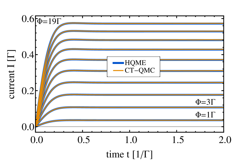
Figure 3: (Color online) Symmetrized current $I=(I_{\text{L}}-I_{\text{R}})/2$ flowing through the impurity at $k_{\text{B}}T=5\Gamma$ as a function of time $t$ for a sequence of equally spaced bias voltages $\Phi=\Gamma,3\Gamma,..,19\Gamma$ where the conduction bands are not shifted with the bias voltage ($S=0$). The model parameters used to obtain this data are summarized in Tab. 1. After a linear increase, the current saturates to a stationary value on a voltage-independent time scale $0.2/\Gamma$. The HQME (blue lines) and CT-QMC methods (orange lines) give identical results to within the numerical resolution of the data.

At lower temperatures, both schemes require a larger computational effort in order to reach the same level of precision as compared to higher temperatures. This is demonstated in Figs. 4 and 5, which show the time-dependent current of our setup at lower temperatures $\beta=1/\Gamma$ and $\beta=5/\Gamma$, respectively. The data has been obtained with a similar numerical effort as that shown in Fig. 3. One observes that both schemes agree very well, but small deviations, which are consistent with the applied accuracy, begin to occur.

As the temperature $T$ decreases, coherent processes become more important and give rise to oscillations of the current level (see Figs. 4 and 5). The period of these oscillations is given by the dynamical phases of the system, in particular the difference between the energy levels of the impurity and the chemical potentials in the electrodes. Accordingly, the dynamical oscillations of the current level show a bias dependence, which is clearly visible in our data. This behavior is known as current ringing and has been outlined before in a slightly different context, namely as a response to bias voltage pulses and/or quenches Wingreen et al. (1993); Taranko et al. (2012).

Another bias dependence appears in the stationary values of the current level. For high temperatures, thermal broadening leads to an almost linear increase of the stationary current, at least in the range of bias voltages considered here. This is evident from the almost equidistant values in Fig. 3. The stationary values seen in Figs. 4 and 5 are clearly non-equidistant. This indicates a strong non-Ohmic saturation of the current level with increasing bias voltage, which originates from the restricted number of conductance channels through the impurity.

We conclude at this point that the agreement between HQME and CT-QMC results is very good in the parameter ranges we have studied. We corroborated this statement for a number of other setups, where we changed the position of the energy levels, $\epsilon_{\uparrow/\downarrow}\neq-U/2$, introduced a level splitting / magnetic field, $\epsilon_{\uparrow}-\epsilon_{\downarrow}\neq 0$, a different shift of the conduction bands, $S=1$ (see below), and different band widths (data not shown). Changing the electron-electron interaction strength, we also observed that the results converge faster for lower values of $U$ (which is consistent with the fact that, for $U=0$, the hierarchy (II.2) terminates at the second tier Jin et al. (2008, 2010)). At lower temperatures, $\beta\gtrsim\beta_{\text{Kondo}}\approx 15/\Gamma$, we were not able to converge the HQME expansion to a satisfactory level.

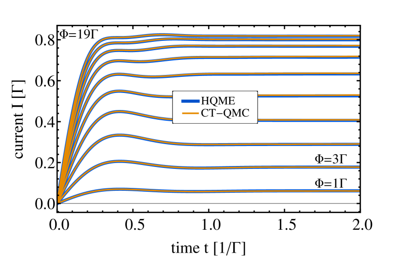
Figure 4: (Color online) Symmetrized current $I=(I_{\text{L}}-I_{\text{R}})/2$ flowing through the impurity at $k_{\text{B}}T=\Gamma$ as a function of time $t$ for a sequence of equally spaced bias voltages $\Phi=\Gamma,3\Gamma,..,19\Gamma$ where the conduction bands are not shifted with the bias voltage ($S=0$). The model parameters used to obtain this data are summarized in Tab. 1. After a linear increase, the current level slightly oscillates before it reaches its stationary value. The corresponding time scales are given by the dynamical phases of the problem and the inverse temperature $1/(k_{\text{B}}T)=1/\Gamma$, respectively.

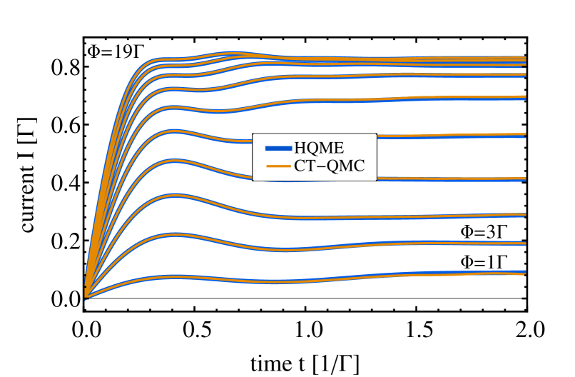
Figure 5: (Color online) Symmetrized current $I=(I_{\text{L}}-I_{\text{R}})/2$ flowing through the impurity at $k_{\text{B}}T=\Gamma/5$ as a function of time $t$ for a sequence of equally spaced bias voltages $\Phi=\Gamma,3\Gamma,..,19\Gamma$ where the conduction bands are not shifted with the bias voltage ($S=0$). The model parameters used to obtain this data are summarized in Tab. 1. The oscillations of the current level that appear right after the initial linear increase become more pronounced at lower temperatures. The corresponding time scales are given by the dynamical phases of the problem and the inverse temperature $1/(k_{\text{B}}T)=\Gamma/5$, respectively. Deviations between the HQME (blue lines) and CT-QMC results (orange lines) are consistent.

Next, we consider electrodes in which the conduction bands are shifted with the applied bias voltage ($S=1$). The time-dependent current of such a system is shown in Fig. 6. It should be compared and contrasted with the data shown in Fig. 4. Two qualitative differences are apparent: the first is that the slope of the current vanishes at $t=0$. This can be easily understood from Eq. (18), as the integral on the right-hand side vanishes for shifted conduction bands. The latter is no longer true for times $t>0$, where, initially, an increase of the current $\sim t^{3}$ is inherited from a change of the populations $\sim t^{2}$ Thoss et al. (2001); Egorova et al. (2003); Härtle and Millis (2014). After this initial phase, the behavior of the unshifted bands is recovered. The other difference is the reduced current level for $e\Phi=19\Gamma$, which falls below the line for $e\Phi=11\Gamma$ at times $t>0.8/\Gamma$. This negative differential resistance originates from both the shift of the conduction bands and their finite band width $D$. This behavior is also well known, for example, from transport through resonant tunneling diodes Davies et al. (1993, 1994).

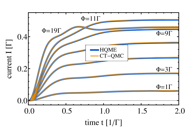
Figure 6: (Color online) Symmetrized current $I=(I_{\text{L}}-I_{\text{R}})/2$ flowing through the impurity at $k_{\text{B}}T=\Gamma$ as a function of time $t$ for a sequence of equally spaced bias voltages $\Phi=\Gamma,3\Gamma,..,11\Gamma$ and $\Phi=19\Gamma$ where the conduction bands are shifted with the bias voltage ($S=1$). The model parameters used to obtain this data are summarized in Tab. 1. In contrast to Figs. 3 – 5, the current level is initially not linearly increasing with the time $t$ when the conduction bands are shifted with the applied bias voltage ($S=1$).

III.3 Evolution of the magnetization for a symmetric and an asymmetric coupling to the electrodes

The HQME method is particularly promising because it allows us to calculate the exact time evolution of a correlated many-body system with a numerical effort that scales linearly with the simulation time. In order to demonstrate this, we discuss the magnetization, as introduced in Eqs. (15). Other observables, like populations or the current, approach their steady state values much faster and are, therefore, less suitable for the present purpose. In addition, we consider an asymmetric coupling to the electrodes. As we will see, the corresponding dynamics shows a richer set of behaviors than in the symmetrically coupled case, and occurs on significantly longer time scales.

We start our analysis with a symmetrically coupled impurity in a strong magnetic field $h=2\Gamma$ (the behavior at other field strengths is similar - data not shown). The corresponding magnetization of the impurity is depicted in Fig. 7 as a function of both bias voltage $\Phi$ and inverse temperature in the electrodes $\beta$. We show a $3\times 3$ array of plots, where the top row represents the magnetization at short time scales, $t=0.5/\Gamma$, and the middle row at intermediate time scales, $t=5/\Gamma$. The bottom row depicts the steady state values. In the latter, we also give the time $t_{0.999}$ at which the impurity reached 99.9% of its final magnetization (note that this time scale is longest for low temperatures and bias voltages). The different columns are obtained using different levels of approximation. The left column is computed using the full HQME approach. The second and third column are obtained by truncating the hierarchy (II.2) at the second and the first tier. This corresponds to a hybridization expansion to $\mathcal{O}((\Gamma/(k_{\text{B}}T))^{2})$ and $\mathcal{O}(\Gamma/(k_{\text{B}}T))$, respectively (see Sec. II.2). The different levels of approximation facilitate a discussion of the relevant processes and mechanisms, for example, where and when processes of higher order are important (see below).

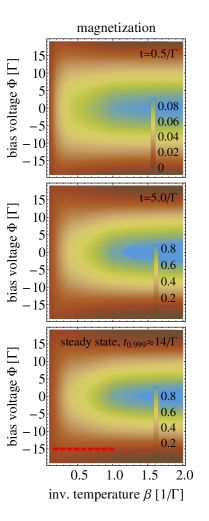
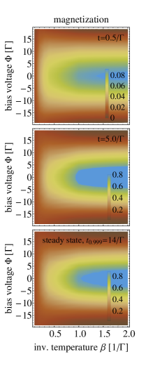
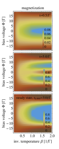
Figure 7: (Color online) Magnetization of an Anderson impurity that is symmetrically coupled to the electrodes as a function of temperature and bias voltage ($S=0$), and for three different times (top row: $t=0.5/\Gamma$; middle row: $t=5/\Gamma$; bottom row: steady state). The left column depicts the full HQME result. The middle and the right column has been obtained by truncating the hierarchy (II.2) at the second and the first tier, respectively. The magnetization along the red dashed line in the lower left plot is also depicted in Fig. 8.

The data of Fig. 7 can be understood as follows. As we start from a state with zero magnetization, the magnetization at short time scales is almost an order of magnitude smaller than the final steady state values. The maximum magnetization is obtained at small bias voltages and temperatures. At higher temperatures and voltages, where the impurity exchanges particles with the electrodes at a wider range of energies, the magnetization becomes quenched. We would like to emphasize that the system reaches its steady state not before times $t\gtrsim 15/\Gamma$.

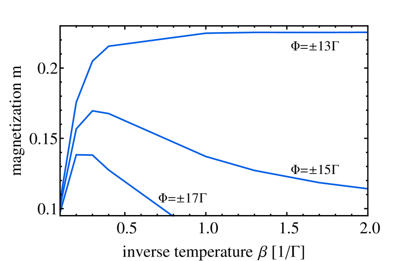
Figure 8: (Color online) Magnetization of an Anderson impurity that is symmetrically coupled to the electrodes as a function of temperature in the steady state and applied bias voltages $\Phi=\pm 13\Gamma$, $\pm 15\Gamma$ and $\pm 17\Gamma$ ($S=0$). Note that the kinks originate from a simple linear interpolation between the data points.

The exact result is very similar to the one that is obtained with a second order truncation of the hierarchy (II.2). A tendency towards a higher magnetization is visible if the number of exchange processes that is taken into account in our calculations is reduced. Truncation at the first tier enhances the effect, but also results in a qualitatively different structure of the magnetization at intermediate time scales (right plot of the middle row). Here, the magnetization shows a peak at positive and negative voltages, while the exact and second order result exhibit only a single peak that is centered around zero bias.

The splitting of the peak magnetization can be understood with the bias dependence of resonant exchange processes with the electrodes. At zero bias, the difference between the chemical potentials in the electrodes and the single-particle levels of the impurity (see Fig. 1b) is largest and resonant processes are strongly suppressed. This suppression is less pronounced at non-zero voltages such that the steady state magnetization can develop on shorter time scales. Accordingly, this behavior shows only a weak temperature dependence, resulting in an almost horizontal splitting of the peak that is seen in Fig. 7. This splitting is not seen at short times scales (right plot of the top row), because the initial state is not decaying exponentially at short times. It rather shows a power-law decay, $\sim t^{2}$, which is well known from an analysis of similar systems in terms of Born-Markov theory Thoss et al. (2001); Egorova et al. (2003); Härtle and Millis (2014).

Another intriguing effect occurs at higher bias voltages ($|e\Phi|>10\Gamma$). Here, the magnetization shows a non-monotonic behavior with respect to temperature: it becomes stabilized by increasing temperature before decreasing again at temperatures $\beta\lesssim 0.2/\Gamma$ (follow, e.g., the red dashed line in Fig. 7 from $\beta=1/\Gamma$ to $\beta=0.1/\Gamma$). This non-monotonic behavior is explicitly depicted in Fig. 8, where the magnetization $m$ is shown, for example, as a function of the inverse temperature $\beta$ and fixed bias voltages $\Phi=\pm 13\Gamma$, $\pm 15\Gamma$ and $\pm 17\Gamma$. This non-linear dependence of the magnetization on temperature was discovered only recently (see Ref. Cohen et al. (2013a)). It is most pronounced in the steady state and for a truncation of the hierarchy (II.2) at a lower tier. The latter points towards a physical interpretation of the effect, suggesting that it originates from the broadening of the peak magnetization around zero bias with increasing temperature and the quenching of the magnetization at very high temperatures.

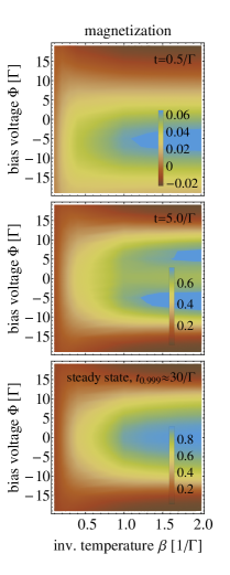
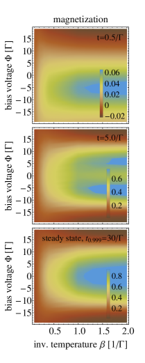
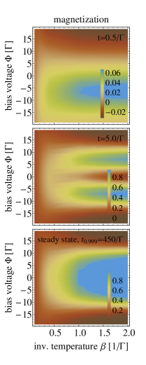
Figure 9: (Color online) Magnetization of an Anderson impurity asymmetrically coupled to the electrodes as a function temperature and bias voltage ($S=0$) and for three different times (top row: $t=0.5/\Gamma$; middle row: $t=5/\Gamma$; bottom row: steady state). The left column depicts the full HQME result. The middle and the right column has been obtained by truncating the hierarchy (II.2) at the second and the first tier, respectively.

The last scenario we discuss is an asymmetric coupling of the impurity to the electrodes. The corresponding magnetization is shown in Fig. 9. It can be directly compared to the magnetization of the symmetrically coupled impurity that is depicted in Fig. 7. It can be seen that, on short time scales (top row), the initial peak of the magnetization is shifted towards negative voltages. This is because the coupling to the right electrode is weaker and we start with an initially unoccupied system. The initial population of the impurity is therefore dominated by exchange processes with respect to the left electrode. The corresponding dynamics occurs on shorter time scales for negative voltages, because the chemical potential of the left electrode $\mu_{\text{L}}$ is then closer to the single-particle levels $\epsilon_{\uparrow/\downarrow}$.

Another qualitative difference with respect to the symmetric case occurs on intermediate time scales. Here, the magnetization is peaked at non-zero values of the bias voltage $\Phi$ even when higher-order processes are taken into account. This behavior was also seen in the symmetric case but only if the hierarchy (II.2) is truncated at the first tier, that is by disregarding higher-order processes. These processes become quenched by the weaker coupling to the right electrode, while resonant processes with respect to the left electrode are not. The situation is therefore similar to the symmetrically coupled case without higher-order processes. The magnetization of the impurity evolves to very similar steady state values, but on even longer times scales ($t\gtrsim 30/\Gamma$). Minor differences occur due to the weaker hybridization with the right electrode (i.e. a less pronounced broadening of the energy levels).

We close this section by a discussion on the generality of our findings. We observed, for example, a very similar behavior of the magnetization dynamics for different choices of the voltage division factor ($\mu_{\text{L}}\neq-\mu_{\text{R}}$ for $\Phi\neq 0$, data not shown). We also calculated the magnetization dynamics starting from different initial states. If, for example, the initial magnetization points in the direction of the magnetic field, the impurity magnetization shows a very similar behavior as compared to the one we discussed for a symmetric coupling to the electrodes. Similar structures as for an asymmetric coupling to the electrodes appear, if the initial magnetization points opposite to the applied magnetic field. These signatures, however, decay on much shorter time scales due to the stronger coupling to the right electrode.

IV Conclusion

In this work, we give the first direct comparison of the hierarchical quantum master equation method Tanimura (2006); Welack et al. (2006); Jin et al. (2008); Härtle et al. (2013); Härtle and Millis (2014) and the diagrammatic, continuous-time quantum Monte Carlo approach Werner et al. (2006, 2009); Schmidt and Komnik (2009); Schiró and Fabrizio (2009); Cohen and Rabani (2011); Cohen et al. (2013a). To this end, we have studied the nonequilibrium transport properties of an Anderson impurity that is coupled to two electrodes with different chemical potentials. This transport problem represents a well established and fairly well understood test case. We discussed the main characteristics of the two numerically exact methods (cf. Sec. II.4). They are distinguished by the range of parameters where exact results can be obtained in practical calculations. CT-QMC gives access to the short- and intermediate-time dynamics ($\lesssim$ 10 units of the inverse hybridization strength) but in general fails to describe long-time dynamics, for example in the presence of Kondo correlations, because the numerical effort scales exponentially with the simulation time Cohen et al. (2013a). In contrast, the hierarchical master equation method scales linearly with the simulation time and is, therefore, not limited in terms of the accessible time scale. It represents a hybridization expansion, which can be carried out to sufficiently high order if the temperature in the electrodes is not too low. For the present problem, we were able to obtain converged results only for temperatures above the Kondo temperature. Our findings provide a wealth of numerically exact benchmark data certain to be useful to future method developers.

We have also elucidated interesting physical phenomena for the range of parameters, where numerically exact results have been accessible with a reasonable numerical effort. We investigated the short-time dynamics of the (symmetrized) current flowing through the impurity in the presence of a bias voltage, starting from a product initial state where the impurity is not populated by electrons. While a linear increase of the current level is found for situations where the conduction bands are not shifted with the applied bias voltage (corresponding to realizations of quantum dots with semiconductor heterostructures), a qualitatively different behavior emerges when the electrodes are not charged when applying a bias voltage. At low temperatures, oscillations of the current level, current ringing Wingreen et al. (1993), due to dynamical phases appear. In addition to the current, we also studied the magnetization dynamics in the presence of a magnetic field. We confirmed the recently reported non-monotonic temperature dependence of the steady state magnetization Cohen et al. (2013a) and traced it back to competing broadening effects of the impurity levels. In addition, we found complex structures on intermediate yet long time scales (i.e., in the cases studied, about 10 units of the inverse hybridization strength) in the presence of an asymmetric coupling to the electrodes (cf. Fig. 9).

Our comparative study is a first step towards practical guidelines in choosing the right solver for a given impurity problem. Since the presented methods cannot cover the full spectrum of problems, it would be interesting to compare them to other exact schemes, including, for example, numerical renormalization group, density matrix renormalization group, multi-layer multi-configurational time-dependent Hartree, or other quantum Monte Carlo schemes. A primary goal is to identify regions of parameter space where methods overlap and, of course, regions which cannot be covered satisfactorily by any of the available methods. Further activities in this direction are planned, and we would like to encourage other researchers to participate in these efforts.

Appendix A Convergence properties of HQME

The convergence properties of the HQME approach strongly depend on the importance criterion that is used to truncate the hierarchy of equations of motion (II.2). In this appendix, we demonstrate the convergence behavior of our HQME scheme explicitly. To this end, we reconsider the time-dependent (converged) current shown in Fig. 4. We replot the result for $\Phi=5\Gamma$ in Fig. 10a. It corresponds to the graph with the threshold value $A_{\text{th}}=10^{-6}$. In addition, we plot results that were obtained for higher threshold values $A_{\text{th}}$. In Tab. 2, we list the number of auxiliary operators (AO) that were taken into account and the maximum tier level. The results are considered to be converged once the threshold value is below $10^{-5}$. The corresponding number of AOs is $\sim 10^{4}$. The respective maximum tier level is $5$.

threshold value		$10^{-1}$			$10^{-2}$			$10^{-3}$			$10^{-4}$			$10^{-5}$			$10^{-6}$
# of AOs		269			447			1158			3009			8317			20912
max. tier level		2			3			3			4			5			5

Table 2: Number of auxiliary operators for different threshold values of the importance criterion (10).

In Sec. III.2, we have shown that our (converged) results coincide with the ones obtained from CT-QMC. This demonstrates the validity and usefulness of our truncation scheme. At this point, we would like to give an additional proof of this statement by showing the convergence of our scheme towards the solution of an analytically solvable case. Fig. 10b has been obtained with the same parameters as Fig. 10b, except that we ’turned off’ electron-electron interactions, i.e. we used $U=0$. In this limit, the exact result is known and can be obtained, for example, by truncating the hierarchy (II.2) at the second tier (without applying the importance criterion (10)) Jin et al. (2008, 2010). It can be seen that our results converge to the exact result and that convergence is faster than in the interacting case.

(a)

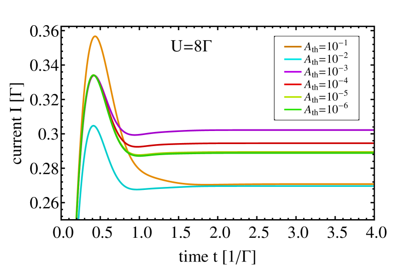
(b)

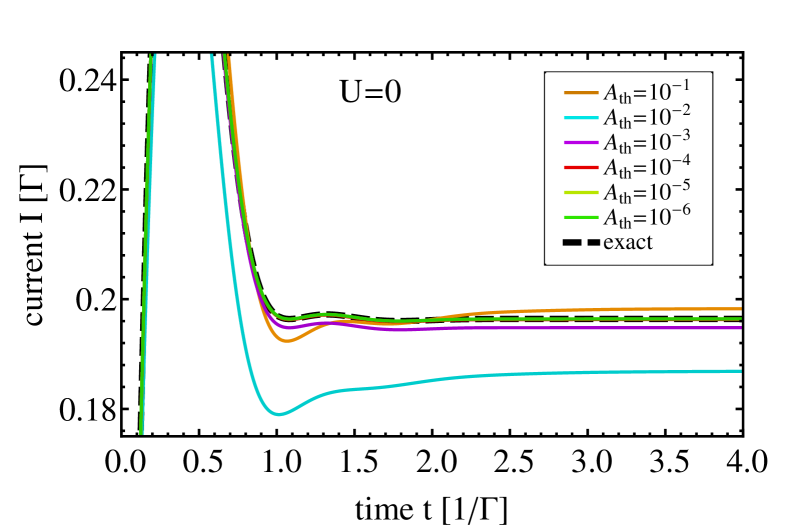
Figure 10: (Color online) Convergence analysis of the symmetrized current $I=(I_{\text{L}}-I_{\text{R}})/2$ that is flowing through the impurity at $k_{\text{B}}T=\Gamma$ and $\Phi=5\Gamma$ ($S=0$) as a function of time $t$. Panel (a) shows the convergence behavior for $U=8\Gamma$. The behavior for $U=0$ is shown in Panel (b). The model parameters used to obtain this data are summarized in Tab. 1.

References

- Andergassen et al. (2010) S. Andergassen, V. Meden, H. Schoeller, J. Splettstoesser, and M. Wegewijs, Nanotechnology 21, 272001 (2010).
- Aoki et al. (2014) H. Aoki, N. Tsuji, M. Eckstein, M. Kollar, T. Oka, and P. Werner, Rev. Mod. Phys. 86, 779 (2014).
- Cuevas and Scheer (2010) J. C. Cuevas and E. Scheer, Molecular Electronics: An Introduction To Theory And Experiment (World Scientific, Singapore, 2010).
- Georges et al. (1996) A. Georges, G. Kotliar, W. Krauth, and M. J. Rozenberg, Rev. Mod. Phys. 68, 13 (1996).
- Freericks et al. (2006) J. K. Freericks, V. M. Turkowski, and V. Zlatić, Phys. Rev. Lett. 97, 266408 (2006).
- Vollhardt (2012) D. Vollhardt, Ann. Phys. (Berlin) 524, 1 (2012).
- Nekrasov et al. (2005) I. A. Nekrasov, G. Keller, D. E. Kondakov, A. V. Kozhevnikov, T. Pruschke, K. Held, D. Vollhardt, and V. I. Anisimov, Phys. Rev. B 72, 155106 (2005).
- Eckstein et al. (2009) M. Eckstein, M. Kollar, and P. Werner, Phys. Rev. Lett. 103, 056403 (2009).
- Tsuji et al. (2013) N. Tsuji, M. Eckstein, and P. Werner, Phys. Rev. Lett. 110, 136404 (2013).
- Joura et al. (2008) A. V. Joura, J. K. Freericks, and T. Pruschke, Phys. Rev. Lett. 101, 196401 (2008).
- Aron et al. (2013) C. Aron, C. Weber, and G. Kotliar, Phys. Rev. B 87, 125113 (2013).
- Freericks (2008) J. K. Freericks, Phys. Rev. B 77, 075109 (2008).
- Eckstein and Werner (2011) M. Eckstein and P. Werner, Phys. Rev. Lett. 107, 186406 (2011).
- Wang et al. (2008) X. Wang, C. D. Spataru, M. S. Hybertsen, and A. J. Millis, Phys. Rev. B 77, 045119 (2008).
- Eckel et al. (2010) J. Eckel, F. Heidrich-Meisner, S. G. Jakobs, M. Thorwart, M. Pletyukhov, and R. Egger, New J. Phys. 12, 043042 (2010).
- Werner et al. (2010) P. Werner, T. Oka, M. Eckstein, and A. J. Millis, Phys. Rev. B 81, 035108 (2010).
- Schmitt and Anders (2010) S. Schmitt and F. B. Anders, Phys. Rev. B 81, 165106 (2010).
- Wang et al. (2011) H. Wang, I. Pshenichnyuk, R. Härtle, and M. Thoss, J. Chem. Phys. 135, 244506 (2011).
- Härtle et al. (2013) R. Härtle, G. Cohen, D. R. Reichman, and A. J. Millis, Phys. Rev. B 88, 235426 (2013).
- Härtle and Millis (2014) R. Härtle and A. J. Millis, Phys. Rev. B 90, 245426 (2014).
- Al-Hassanieh et al. (2006) K. A. Al-Hassanieh, A. E. Feiguin, J. A. Riera, C. A. Büsser, and E. Dagotto, Phys. Rev. B 73, 195304 (2006).
- Dias da Silva et al. (2008) L. G. G. V. Dias da Silva, F. Heidrich-Meisner, A. E. Feiguin, C. A. Büsser, G. B. Martins, E. V. Anda, and E. Dagotto, Phys. Rev. B 78, 195317 (2008).
- Kirino et al. (2008) S. Kirino, T. Fujii, J. Zhao, and K. Ueda, J. Phys. Soc. Jpn. 77, 084704 (2008).
- Heidrich-Meisner et al. (2009) F. Heidrich-Meisner, A. E. Feiguin, and E. Dagotto, Phys. Rev. B 79, 235336 (2009).
- Kirino et al. (2010) S. Kirino, T. Fujii, and K. Ueda, Physica E 42, 874 (2010).
- Branschädel et al. (2010) A. Branschädel, G. Schneider, and P. Schmitteckert, Ann. Phys. 522, 657 (2010).
- Anders (2008a) F. B. Anders, Phys. Rev. Lett. 101, 066804 (2008a).
- Anders (2008b) F. B. Anders, J. Phys.: Condens. Matter 20, 195216 (2008b).
- Wang and Thoss (2013) H. Wang and M. Thoss, J. Chem. Phys. 138, 134704 (2013).
- Balzer et al. (2015) K. Balzer, Z. Li, O. Vendrell, and M. Eckstein, Phys. Rev. B 91, 045136 (2015).
- Žitko and Pruschke (2009) R. Žitko and T. Pruschke, Phys. Rev. B 79, 085106 (2009).
- Weiss et al. (2008) S. Weiss, J. Eckel, M. Thorwart, and R. Egger, Phys. Rev. B 77, 195316 (2008).
- Segal et al. (2010) D. Segal, A. J. Millis, and D. R. Reichman, Phys. Rev. B 82, 205323 (2010).
- Segal et al. (2011) D. Segal, A. J. Millis, and D. R. Reichman, Phys. Chem. Chem. Phys. 13, 14378 (2011).
- Hützen et al. (2012) R. Hützen, S. Weiss, M. Thorwart, and R. Egger, Phys. Rev. B 85, 121408 (2012).
- Weiss et al. (2013) S. Weiss, R. Hützen, D. Becker, J. Eckel, R. Egger, and M. Thorwart, Phys. Status Solidi B 250, 2298 (2013).
- Werner et al. (2006) P. Werner, A. Comanac, L. de’ Medici, M. Troyer, and A. J. Millis, Phys. Rev. Lett. 97, 076405 (2006).
- Schmidt et al. (2008) T. L. Schmidt, P. Werner, L. Mühlbacher, and A. Komnik, Phys. Rev. B 78, 235110 (2008).
- Werner et al. (2009) P. Werner, T. Oka, and A. J. Millis, Phys. Rev. B 79, 035320 (2009).
- Schiró (2010) M. Schiró, Phys. Rev. B 81, 085126 (2010).
- Gull et al. (2011a) E. Gull, A. J. Millis, A. I. Lichtenstein, A. N. Rubtsov, M. Troyer, and P. Werner, Rev. Mod. Phys. 83, 349 (2011a).
- Mühlbacher et al. (2011) L. Mühlbacher, D. F. Urban, and A. Komnik, Phys. Rev. B 83, 075107 (2011).
- Cohen et al. (2013a) G. Cohen, E. Gull, D. R. Reichman, A. J. Millis, and E. Rabani, Phys. Rev. B 87, 195108 (2013a).
- Cohen and Rabani (2011) G. Cohen and E. Rabani, Phys. Rev. B 84, 075150 (2011).
- Zheng et al. (2009) X. Zheng, J. Jin, S. Welack, M. Luo, and Y. Yan, J. Chem. Phys. 130, 164708 (2009).
- Paaske and Flensberg (2005) J. Paaske and K. Flensberg, Phys. Rev. Lett. 94, 176801 (2005).
- Mühlbacher and Rabani (2008) L. Mühlbacher and E. Rabani, Phys. Rev. Lett. 100, 176403 (2008).
- Schmidt and Komnik (2009) T. L. Schmidt and A. Komnik, Phys. Rev. B 80, 041307 (2009).
- Schiró and Fabrizio (2009) M. Schiró and M. Fabrizio, Phys. Rev. B 79, 153302 (2009).
- Tanimura (2006) Y. Tanimura, J. Phys. Soc. Jpn. 75, 082001 (2006).
- Welack et al. (2006) S. Welack, M. Schreiber, and U. Kleinekathöfer, J. Chem. Phys. 124, 044712 (2006).
- Jin et al. (2008) J. Jin, X. Zheng, and Y. Yan, J. Chem. Phys. 128, 234703 (2008).
- Cronenwett et al. (1998) S. M. Cronenwett, T. H. Oosterkamp, and L. P. Kouwenhoven, Science 281, 540 (1998).
- Goldhaber-Gordon et al. (1998) D. Goldhaber-Gordon, H. Shtrikman, D. Mahalu, D. Abusch-Magder, U. Meirav, and M. A. Kastner, Nature 391, 156 (1998).
- Liang et al. (2002) W. Liang, M. Shores, M. Bockrath, J. Long, and H. Park, Nature (London) 417, 725 (2002).
- Pasupathy et al. (2004) A. N. Pasupathy, R. C. Bialczak, J. Martinek, J. E. Grose, L. A. K. Donev, P. L. McEuen, and D. C. Ralph, Science 306, 86 (2004).
- Osorio et al. (2007) E. A. Osorio, K. O’Neill, M. Wegewijs, N. Stuhr-Hansen, J. Paaske, T. Bjørnholm, and H. S. J. van der Zant, Nano Lett. 7, 3336 (2007).
- Roch et al. (2008) N. Roch, S. Florens, V. Bouchiat, W. Wernsdorfer, and F. Balestro, Nature 453, 633 (2008).
- Yu et al. (2004) L. H. Yu, Z. K. Keane, J. W. Ciszek, L. Cheng, M. P. Stewart, J. M. Tour, and D. Natelson, Phys. Rev. Lett. 93, 266802 (2004).
- Sapmaz et al. (2005) S. Sapmaz, P. Jarillo-Herrero, Y. M. Blanter, and H. S. J. van der Zant, New J. Phys. 7, 243 (2005).
- Pasupathy et al. (2005) A. N. Pasupathy, J. Park, C. Chang, A. V. Soldatov, S. Lebedkin, R. C. Bialczak, J. E. Grose, L. A. K. Donev, J. P. Sethna, D. C. Ralph, and P. L. McEuen, Nano Lett. 5, 203 (2005).
- Thijssen et al. (2006) W. H. A. Thijssen, D. Djukic, A. F. Otte, R. H. Bremmer, and J. M. van Ruitenbeek, Phys. Rev. Lett. 97, 226806 (2006).
- Parks et al. (2007) J. J. Parks, A. R. Champagne, G. R. Hutchison, S. Flores-Torres, H. D. Abruna, and D. C. Ralph, Phys. Rev. Lett. 99, 026601 (2007).
- Böhler et al. (2007) T. Böhler, A. Edtbauer, and E. Scheer, Phys. Rev. B 76, 125432 (2007).
- de Leon et al. (2008) N. P. de Leon, W. Liang, Q. Gu, and H. Park, Nano Lett. 8, 2963 (2008).
- Repp et al. (2010) J. Repp, P. Liljeroth, and G. Meyer, Nature Physics 6, 975 (2010).
- Ballmann et al. (2010) S. Ballmann, W. Hieringer, D. Secker, Q. Zheng, J. A. Gladysz, A. Görling, and H. B. Weber, ChemPhysChem 11, 2256 (2010).
- Ballmann et al. (2012) S. Ballmann, R. Härtle, P. B. Coto, M. Elbing, M. Mayor, M. R. Bryce, M. Thoss, and H. B. Weber, Phys. Rev. Lett. 109, 056801 (2012).
- Ballmann et al. (2013) S. Ballmann, W. Hieringer, R. Härtle, P. B. Coto, M. R. Bryce, A. Görling, M. Thoss, and H. B. Weber, Phys. Status Solidi B 250, 2452 (2013).
- Hu et al. (2010) J. Hu, R. Xu, and Y. Yan, J. Chem. Phys. 133, 101106 (2010).
- Hu et al. (2011) J. Hu, M. Luo, F. Jiang, R. Xu, and Y. Yan, J. Chem. Phys. 134, 244106 (2011).
- Jin et al. (2010) J. Jin, M. W. Tu, W. Zhang, and Y. Yan, New J. Phys. 12, 083013 (2010).
- Anders and Schiller (2005) F. B. Anders and A. Schiller, Phys. Rev. Lett. 95, 196801 (2005).
- Wang and Thoss (2009) H. Wang and M. Thoss, J. Chem. Phys. 131, 024114 (2009).
- Gull et al. (2011b) E. Gull, D. R. Reichman, and A. J. Millis, Phys. Rev. B 84, 085134 (2011b).
- Simine and Segal (2013) L. Simine and D. Segal, J. Chem. Phys. 138, 214111 (2013).
- Wilner et al. (2013) E. Y. Wilner, H. Wang, G. Cohen, M. Thoss, and E. Rabani, Phys. Rev. B 88, 045137 (2013).
- Wolf et al. (2014) F. A. Wolf, I. P. McCulloch, and U. Schollwöck, Phys. Rev. B 90, 235131 (2014).
- Wang et al. (2015) P. Wang, G. Cohen, and S. Xu, Phys. Rev. B 91, 155148 (2015).
- Cohen et al. (2014a) G. Cohen, D. R. Reichman, A. J. Millis, and E. Gull, Phys. Rev. B 89, 115139 (2014a).
- Gull et al. (2010) E. Gull, D. R. Reichman, and A. J. Millis, Phys. Rev. B 82, 075109 (2010).
- Cohen et al. (2013b) G. Cohen, E. Y. Wilner, and E. Rabani, New J. Phys. 15, 073018 (2013b).
- Cohen et al. (2014b) G. Cohen, E. Gull, D. R. Reichman, and A. J. Millis, Phys. Rev. Lett. 112, 146802 (2014b).
- Eckstein and Werner (2010) M. Eckstein and P. Werner, Phys. Rev. B 82, 115115 (2010).
- Rüegg et al. (2012) A. Rüegg, E. Gull, D. R. Reichman, and A. J. Millis, arXiv:1212.2694 (2012).
- Tsvelick and Wiegmann (1982) A. M. Tsvelick and P. B. Wiegmann, Physics Letters 89A, 157 (1982).
- Wingreen et al. (1993) N. S. Wingreen, A. P. Jauho, and Y. Meir, Phys. Rev. B 48, 8487 (1993).
- Taranko et al. (2012) E. Taranko, M. Wiertel, and R. Taranko, J. Appl. Phys. 111, 023711 (2012).
- Thoss et al. (2001) M. Thoss, H. Wang, and W. H. Miller, J. Chem. Phys. 115, 2991 (2001).
- Egorova et al. (2003) D. Egorova, M. Thoss, W. Domcke, and H. Wang, J. Chem. Phys. 119, 2761 (2003).
- Davies et al. (1993) J. H. Davies, S. Hershfield, P. Hyldgaard, and J. W. Wilkins, Phys. Rev. B 47, 4603 (1993).
- Davies et al. (1994) J. H. Davies, S. Hershfield, P. Hyldgaard, and J. W. Wilkins, Ann. Phys. (NY) 236, 1 (1994).