Ultrarelativistic (Cauchy) spectral problem in the infinite well

Abstract

We analyze spectral properties of the ultrarelativistic (Cauchy) operator $|\Delta|^{1/2}$, provided its action is constrained exclusively to the interior of the interval $[-1,1]\subset R$. To this end both analytic and numerical methods are employed. New high-accuracy spectral data are obtained. A direct analytic proof is given that trigonometric functions $\cos(n\pi x/2)$ and $\sin(n\pi x)$, for integer $n$ are not the eigenfunctions of $|\Delta|_{D}^{1/2}$, $D=(-1,1)$. This clearly demonstrates that the traditional Fourier multiplier representation of $|\Delta|^{1/2}$ becomes defective, while passing from $R$ to a bounded spatial domain $D\subset R$.

I Introduction

Fractional (Lévy-type) operators are known to be spatially nonlocal. This becomes an issue if confronted with a priori imposed exterior Dirichlet boundary data, which set the familiar (quantum) infinite well enclosure. Standard fractional Laplacians, at each instant of time, extend their nonlocal action to the entire real axis $R$ and this property needs to be reconciled with the finite support $D=(-1,1)\subset R$ of the infinite well with width equal $2$.

One of the obvious obstacles arising here is rooted in the fact, that the traditional Fourier multiplier representation of Lévy operators is no longer operational in the finite interval, GS -getoor , see specifically pgar ; zg . Compare e.g. also a discussion of that issue for the familiar (Laplacian-generated) quantum mechanical infinite well problem, see e.g. karwowski ; robinett and zg .

To elucidate the above point, let us recall that the Fourier integral ${\frac{1}{\sqrt{2\pi}}}\int_{R}|k|^{\mu}\tilde{f}(k)e^{-\imath kx}dk=-\partial_{\mu}f(x)/\partial|x|^{\mu}=|\Delta|^{\mu/2}f(x)$, where $\tilde{f}$ stands for a Fourier transform of $f\in L^{2}(R)$ and $g(k)=|k|^{\mu}\tilde{f}(k)$ is presumed to be $L^{2}(R)$-integrable. It is $|k|^{\mu}$ which plays the role of the pertinent Fourier multiplier.

The above Fourier formula is quite often interpreted as a universal definition of both the fractional operator $-|\Delta|^{\mu/2}$ and that of the fractional derivative of the $\mu$-th order, $\partial_{\mu}f(x)/\partial|x|^{\mu}=-|\Delta|^{\mu/2}f(x)$, for $\mu\in(0,2)$. However, this definition is unquestionably valid only, if the fractional operator is defined on the whole real line $R$. More than that, it appears to be merely a specific admissible choice in the family of equivalent (while on $R$) definitions, ten .

The nonlocal operator $-|\Delta|^{\mu/2}$, is known to generate two versions of so-called fractional dynamics (dimensional constants being scaled away): (i) the semigroup $\exp(-t|\Delta|^{\mu/2})\,f$ and (ii) unitary $\exp(-it|\Delta|^{\mu/2})\,f$ ones.

Apart from the unperturbed (free) case, the Fourier (multiplier) representation of the fractional dynamics has proved useful if an infinite or periodic support is admitted for functions in the domain, ZRK . For the simplest quadratic ($\sim x^{2}$) perturbation of the fractional Laplacian (the fractional oscillator problem), a complete analytic solution has been found in the ultrarelativistic (Cauchy) oscillator case, by resorting to Fourier space (and Fourier multiplier) methods.

For more complicated perturbations, and likewise for a deceivingly simple problem of the fractional Laplacian in a bounded (spatial) domain, standard Fourier techniques have been found to be of a doubtful or limited use, ZRK . Therefore, to keep spatial constraints under control, we turn over to a fully-fledged spatially nonlocal definition of the fractional Laplacian, that is well known in the mathematical and statistical physics literature ZG -K , while seldom invoked by quantum theory practitioners, see however GS and references there in.

Dating back to the classic papers riesz ; hadamard , one interprets the fractional Laplacian $-|\Delta|^{\mu/2}$, $\mu\in(0,2)$ as a pseudo-differential (integral) spatially nonlocal operator and its action on a function from the $L^{2}(R)$ domain is commonly defined by employing the Cauchy principal value of the involved integral (evaluated relative to singular points of integrands)

$$|\Delta|^{\mu/2}f(x)\,=\,-{\frac{\Gamma(\mu+1)\sin(\pi\mu/2)}{\pi}}\int_{R}{\frac{f(z)-f(x)}{|z-x|^{1+\mu}}}\,dz.$$ (1)

For a rationale and a broader discussion of the uses (and misuses) of this formula, including its Fourier multiplier version, see GS .

By departing from the general spatially nonlocal definition (1) we shall pass to the specialized Cauchy case ($\mu=1$) of the fractional Laplacian and next focus our attention on its properties under exterior Dirichlet boundary data (e.g. the infinite well enclosure). This issue has received some coverage in the literature, both physics-oriented ZG -ZRK and purely mathematical getoor -dyda . See also Ref. GS for additional references and a discussion of earlier attempts to find the spectral solution for the infinite fractional well.

In the present paper, the term ”ultrarelativistic” directly stems form the notion of the quasi-relativistic operator $\sqrt{-\Delta+m^{2}}$ (natural units being presumed) and its mass $m\rightarrow 0$ limit $|\Delta|^{1/2}$, see e.g. GS and rel .

II The infinite well enclosure: From $|\Delta|^{1/2}$ to $|\Delta|_{D}^{1/2}$.

The Hamiltonian-type expression $H=-|\Delta|^{1/2}+V$, with $V(x)=0$ for $x\in D=(-1,1)\subset R$, is an encoding of the Cauchy operator with the Dirichlet boundary conditions (so-called zero exterior condition on $R\setminus D$) imposed on $L^{2}(R)$ functions $f(x)$ in the domain of $H$: $f(x)=0$ for $|x|\geq 1$. We point out that the Cauchy operator $|\Delta|^{1/2}$ if restricted to a domain comprising solely $L^{2}(R)$ functions with a support in $D$ and vanishing on $R\backslash D$ is not a self-adjoint operator in $L^{2}(R)$.

However, if we consider the action of $|\Delta|^{1/2}$ on test functions $f\in C_{0}^{\infty}(D)$ (infinitely differentiable functions that are compactly supported in $R$ ), then the restriction $|\Delta|^{1/2}_{D}$ of $|\Delta|^{1/2}$ to $D$ is interpreted as the Cauchy operator with the zero (Dirichlet) exterior condition on $R\backslash D$ and is known to extend to a self-adjoint operator in $L^{2}(D)$, K . The passage from $C_{0}^{\infty}(R)$ to $C_{0}^{\infty}(D)$ ultimately amounts to disregarding any $R\backslash D$ contribution implicit in the formal definition (1).

Let us discuss the $D$ versus $R\backslash D$ interplay in more detail, by considering the action of $|\Delta|^{1/2}$ on these $C_{0}^{\infty}(R)$ functions which are actually supported in $D$, i.e. $\psi\in C_{0}^{\infty}(D)$, while departing from the original nonlocal definition:

$$|\Delta|^{1/2}\psi(x)=-\frac{1}{\pi}\int_{R}\frac{\psi(x+y)-\psi(x)}{y^{2}}dy.$$ (2)

$$\psi(x)=\left\{\begin{array}[]{c}\psi(x),\ x\in(-1,1)\\ 0,\quad{\rm{otherwise}},\end{array}\right.$$ (3)

Given $x\in(-1,1)$, we realize that $\psi(x+y)$ does not vanish identically if $x+y\in(-1,1)$ i.e. for $-1-x<y<1-x$. Therefore, the integration (2) can be simplified by decomposing $R$ into $(-\infty<y\leq-1-x)\cup(-1-x<y<1-x)\cup(1-x\leq y<\infty)$. We have:

$$|\Delta|^{1/2}\psi=-\frac{1}{\pi}\left[-\psi(x)\left(\int_{-\infty}^{-1-x}\frac{dy}{y^{2}}+\int_{1-x}^{\infty}\frac{dy}{y^{2}}\right)+\int_{-1-x}^{1-x}\frac{\psi(x+y)-\psi(x)}{y^{2}}dy\right]=$$

$$=\frac{2}{\pi}\frac{\psi(x)}{1-x^{2}}-\frac{1}{\pi}\int_{-1-x}^{1-x}\frac{\psi(x+y)-\psi(x)}{y^{2}}dy,$$ (4)

where the second integral should be understood as the Cauchy principal value with respect to $0$, i.e. $\int_{-1-x}^{1-x}=\lim_{\varepsilon\to 0}\left[\int_{-1-x}^{-\varepsilon}+\int_{-\varepsilon}^{1-x}\right]$.

Given $x\in(-1,1)$, let us make a substitution $x+y=t$ in (4), presuming that now the Cauchy principal value needs to be evaluated relative to $x$. We obtain (note the principal value $(p.v.)$ symbol, introduced in the self-explanatory notation)

$$|\Delta|^{1/2}\psi=\frac{2}{\pi}\frac{\psi(x)}{1-x^{2}}+\frac{1}{\pi}\int_{-1}^{1}\frac{\psi(x)-\psi(t)}{(t-x)^{2}}dt=\frac{2}{\pi}\frac{\psi(x)}{1-x^{2}}+\frac{1}{\pi}(p.v.)\left[\left.-\frac{\psi(x)}{t-x}\right|_{-1}^{1}-\int_{-1}^{1}\frac{\psi(t)dt}{(t-x)^{2}}\right]=$$

$$=\frac{1}{\pi}\,\lim_{\epsilon\rightarrow 0}\left[{\frac{2\psi(x)}{\epsilon}}-\int_{-1}^{{x-\epsilon}}\frac{\psi(t)dt}{(t-x)^{2}}-\int_{x+\epsilon}^{1}{\frac{\psi(t)dt}{(t-x)^{2}}}\right]\equiv-\frac{1}{\pi}({\cal{H}})\int_{-1}^{1}\frac{\psi(t)dt}{(t-x)^{2}},$$ (5)

where $({\cal{H}})$ refers to the Hadamard regularization of hypersingular integrals (Hadamard finite part, extensively employed in the engineering literature, hadamard -klerk ). We point out that the troublesome term $\frac{2}{\pi}\frac{\psi(x)}{1-x^{2}}$ has been cancelled away by its negative coming from the evaluation of $(p.v.)[...]$ in the above.

The second line of the formula (5) can be interpreted as a definition of $|\Delta|^{1/2}_{D}$. The pertinent operator, instead of referring merely to $C_{0}^{\infty}(D)$ functions, can be literally applied (extended) to functions $\psi\in L^{2}(D)$.

In the literature on the usage of the Hadamard finite part evaluation of hypersingular integrals, it is often mentioned that if the $({\cal{H}})$ integral and the $(p.v.)$ integrals in question do exist, we can relate them as follows:

$$|\Delta|^{1/2}_{D}\psi(x)=-\frac{1}{\pi}\,({\cal{H}})\int_{-1}^{1}\frac{\psi(t)dt}{(t-x)^{2}}=-\frac{1}{\pi}\,{\frac{d}{dx}}(p.v.)\int_{-1}^{1}{\frac{\psi(t)dt}{t-x}}.$$ (6)

We shall employ another version of the Hadamard - Cauchy integral relation, by following a direct integration by parts procedure and continually keeping in mind that the involved integrals are (hyper)singular, c.f. also klerk ; monegato .

Namely, by invoking the second line of Eq. (5) and performing integrations by parts before the limit $\epsilon\rightarrow 0$ is ultimately taken, we end up with:

$$|\Delta|^{1/2}_{D}\psi(x)=-\frac{1}{\pi}\,({\cal{H}})\int_{-1}^{1}\frac{\psi(t)dt}{(t-x)^{2}}=-\frac{1}{\pi}\,(p.v.)\int_{-1}^{1}\frac{\psi^{\prime}(t)dt}{t-x},$$ (7)

where $\psi^{\prime}(t)=d\psi(t)/dt$.

We are interested in solving an eigenvalue problem $|\Delta|^{1/2}_{D}\psi=E\,\psi$ for the infinite Cauchy well, while interpreted in terms of the hypersingular integral equation. For explicit computations we shall employ the Hadamard (finite part)-Cauchy (principal value) relation (7):

$$E\,\psi(x)+\frac{1}{\pi}\,(p.v.)\int_{-1}^{1}\frac{\psi^{\prime}(t)dt}{t-x}=0.$$ (8)

III $\cos(\pi x/2)$ and $\sin(\pi x)$ are not eigenfunctions of $|\Delta|^{1/2}_{D}$.

In Ref. GS we have discussed the validity of counter-arguments against proposed so-far, in the physical literature, spectral solutions for Lévy-stable infinite well problems jeng ; luchko . By invoking rigorous mathematical results of K ; KKMS we have given in ZG ; zg the computer-assisted proofs (elaborated for the infinite Cauchy well) that spectral results of laskin -iomin are surely incorrect in the lower part of the spectrum and may be employed at most as approximate expressions for higher eigenvalues. In particular a computer-assisted analysis of approximate eigenfunctions shapes zg have demonstrated quite clearly that ”plain” trigonometric functions (like e.g. sine and cosine) are not the eigenfunctions for the problem under consideration, see also luchko .

Presently we shall demonstrate analytically that $\cos(\pi x/2)$ is not the ground state function of $|\Delta|^{1/2}_{D}$, so contradicting claims of bayin ; bayin1 ; iomin . Our method is different from that adopted in Ref luchko . The integrations are to be performed in the Hadamard sense, c.f. (5) and that will allow us to introduce basic tools that will be necessary in the subsequent more general spectral analysis.

Let us directly substitute $\psi(x)=\cos(\pi x/2)$ to Eq.(6). We shall demonstrate that:

$$|\Delta|^{1/2}_{D}\cos\frac{\pi x}{2}=-\frac{1}{\pi}({\cal{H}})\int_{-1}^{1}\frac{\cos\frac{\pi t}{2}dt}{(t-x)^{2}}=\frac{1}{2}\cos\frac{\pi x}{2}\left[{\mathrm{Si}}\frac{\pi(1+x)}{2}+{\mathrm{Si}}\frac{\pi(1-x)}{2}\right]+\frac{1}{2}\sin\frac{\pi x}{2}\left[{\mathrm{Ci}}\frac{\pi(1-x)}{2}-{\mathrm{Ci}}\frac{\pi(1+x)}{2}\right],$$ (9)

which surely remains incompatible with any function of the form $E\,\cos(\pi x/2)$, where $E>0$ is a constant and $x\in(-1,1)$. Here ${\mathrm{Ci}}(x)$ and ${\mathrm{Si}}(x)$ are respectively the cosine and sine integral functions, which are defined as follows, abr :

$${\mathrm{Si}}(x)=\int_{0}^{x}\frac{\sin t}{t}dt=\frac{1}{\pi}-\int_{x}^{\infty}\frac{\sin t}{t}dt$$ (10)

is an entire function on $R$ with the properties ${\mathrm{Si}}(\infty)=\pi/2$ and ${\mathrm{Si}}(-x)=-{\mathrm{Si}}(x)$, while

$${\mathrm{Ci}}(x)=-\int_{x}^{\infty}\frac{\cos t}{t}dt=C+\ln x+\int_{0}^{x}\frac{\cos t-1}{t}dt$$ (11)

is restricted to $R^{+}$and $C=-\int_{0}^{\infty}e^{-t}\ln t\,dt=0.577215665...$ stands for the Euler-Mascheroni constant.

We point out that ${\mathrm{Si}}(x)$ is defined everywhere on $R$ as a continuous and differentiable function. On the contrary, ${\mathrm{Ci}}(x)$, $x\in R^{+}$ logarithmically escapes towards $-\infty$ as $x$ drops down to $0$ abr ; GR . In the vicinity of the well boundaries $x\to\pm 1$ of $D$, the logarithmic divergence $\ln(1-|x|)\to-\infty$ definitely dominates.

For the direct evaluation of $|\Delta|^{1/2}_{D}\cos\frac{\pi x}{2}$, with $x\in(-1,1)$ we shall employ the Cauchy principal value formula (7). According to Eq. (7), we have:

$$|\Delta|^{1/2}_{D}\cos(\frac{\pi x}{2})={\frac{1}{2}}(p.v.)\int_{-1}^{1}\frac{\sin(\pi t/2)}{t-x}dt={\frac{1}{2}}(p.v.)\int_{-1-x}^{1-x}\frac{\sin[\pi(u+x)/2]}{u}du=$$ (12)

$$+{\frac{1}{2}}\cos(\pi x/2)\,(p.v.)\int_{-1-x}^{1-x}{\frac{\sin(\pi u/2)}{u}}du+{\frac{1}{2}}\sin(\pi x/2)(p.v.)\int_{-1-x}^{1-x}{\frac{\cos(\pi u/2)}{u}}du.$$

By employing the definition (10), we readily get

$$(p.v.)\int_{-1-x}^{1-x}{\frac{\sin(\pi u/2)}{u}}du=\lim_{\epsilon\downarrow 0}\left[\int_{-1-x}^{-\epsilon}+\int^{1-x}_{\epsilon}\right]{\frac{\sin(\pi u/2)}{u}}du={\mathrm{Si}}{\frac{\pi(1+x)}{2}}+{\mathrm{Si}}{\frac{\pi(1-x)}{2}}.$$ (13)

To evaluate $(p.v.)\int_{-1-x}^{1-x}{\frac{\cos(\pi u/2)}{u}}du$, let us notice that

$$(p.v.)\int_{-1-x}^{1-x}{\frac{\cos(\pi u/2)-1}{u}}du=\lim_{\epsilon\downarrow 0}\left[\int_{-1-x}^{-\epsilon}+\int^{1-x}_{\epsilon}\right]{\frac{\cos(\pi u/2)-1}{u}}du=\ln{\frac{1+x}{1-x}}+\left[\int_{0}^{1+x}-\int_{0}^{1-x}\right]{\frac{\cos(\pi u/2)}{u}}du.$$ (14)

By employing (11), we get

$$(p.v.)\int_{-1-x}^{1-x}{\frac{\cos(\pi u/2)}{u}}du={\mathrm{Ci}}(1-x)-{\mathrm{Ci}}(1+x)$$ (15)

and the identity (9) readily follows. Clearly, the outcome (9) is incompatible with $E\,\cos(\pi x/2)$, $E>0$, as predicted in laskin , bayin ; bayin1 ; iomin )

With all necessary tools in hands, one can easily verify that the the lowest odd would-be (candidate) eigenfunction $\sin(\pi x)$ (that according to laskin , bayin ; bayin1 ; iomin ) of $|\Delta|^{1/2}_{D}$ is a faulty guess. Namely, we have:

$$|\Delta|^{1/2}_{D}\sin(\pi x)=-\frac{1}{\pi}({\cal{H}})\int_{-1}^{1}\frac{\sin\pi t}{(t-x)^{2}}dt=\sin(\pi x)\Bigl{(}{\rm{Si}}[\pi(1-x)]+{\rm{Si}}[\pi(1+x)]\Bigr{)}-\cos(\pi x)\Bigl{(}{\rm{Ci}}[\pi(1-x)]-{\rm{Ci}}[\pi(1+x)]\Bigr{)},$$ (16)

while an expected outcome (according to laskin , bayin ; bayin1 ; iomin ) should be $E^{\prime}\,\sin(\pi x)$, where $E^{\prime}>0$ is a constant. This is definitely not the case. We point out that a logarithmic divergence becomes dominant at the boundaries of the interval $D$, that in view of ${\rm{Ci}}[\pi(1-x)]\rightarrow-\infty$ for $x\uparrow 1$ and $-{\rm{Ci}}[\pi(1+x)]\rightarrow+\infty$ as $x\downarrow-1$.

The above discussion easily extends to more general formulas (23) and (36) in below, which provide a direct analytic demonstration that trigonometric functions of the form $\cos(n\pi x/2)$ and $\sin(n\pi x/2)$ with $n$ integer, are not the eigenfunctions of $|\Delta|^{1/2}_{D}$. That invalidates claims to the contrary, appearing in the literature on so-called fractional quantum mechanics, laskin , bayin ; bayin1 ; iomin .

We note that on formal grounds, the trigonometric functions seem to be valid eigenfunctions if the Fourier multiplier representation (c.f. Section I) is ”blindly” used, ignoring the subtleties related to Fourier integrals of functions with support in a bounded domain, ZG ; karwowski ; robinett . The point is that the primary, mathematically well founded, definition of the fractional operator is provided by the integral formula (1) and not by its Fourier integral version. The latter is merely a derived one while on $R$, ten . If spatial constraints are imposed, we may keep their effects under tight control only on the level of Eq. (1), see our considerations of Section II.

IV Solution of the eigenvalue problem in the infinite ultrarelativistic well

Now we are going to solve the integral equation (8), i.e. to deduce the eigenfunctions and eigenvalues of the nonlocal operator $|\Delta|^{1/2}_{D}$. We note pol that there are no worked out systematic methods (even numerical) of solution of integral equations if their kernels are singular, or (that is worse) hypersingular. In below we shall provide an example of a successful solution method, based on Fourier series (trigonometric) expansion in $L^{2}(D)$. Derivations of approximate eigenfunctions and eigenvalues are computer-assisted. The outcomes converge slowly towards ”true” solutions due to the singular behavior of ${\rm{Ci}}$ at the boundaries of $D$.

To find the eigenfunctions and eigenvalues of the nonlocal operator $|\Delta|^{1/2}_{D}$, we adopt the following assumptions:

• Based on standard quantum mechanical (Laplacian based) infinite well experience and previous attempts, K ; KKMS and ZG -zg , to solve the Lévy-stable infinite well problem we can safely classify eigenfunctions to be odd or even. The oscillation theorem appears here to be valid and the ground state has no nodes (intersections with $x$ axis), first excited state has one node, second one has two nodes etc. So, our even states can be labeled by quantum numbers $k=$ 0,2,4,6,… while odd states by $k=$1,3,5,….

• The (Hilbert) state space of the system can be interpreted as a direct sum of odd and even (sub)spaces, equipped with basis systems comprising respectively even and odd orthonormal sets of functions in the interval [-1,1].

• In accordance with the infinite well boundary conditions, the function in the domain of $|\Delta|^{1/2}_{D}$ must obey $\psi(x)=0$ for $|x|\geq 1$. In consequence, among various orthogonal sets available in $L^{2}(D)$, we are ultimately left with standard trigonometric functions.

• The even basis system in $L^{2}(D)$ is composed of cosines

  $$\varphi_{k}(x)=\cos\frac{(2k+1)\pi x}{2},\quad\int_{-1}^{1}\varphi_{k}(x)\varphi_{l}(x)dx=\delta_{kl},\quad k\geq 0,$$ (17)

  where $\delta_{kl}$ is the Kronecker symbol. For the odd basis system we take the sines

  $$\chi_{k}(x)=\sin k\pi x,\quad\int_{-1}^{1}\chi_{k}(x)\chi_{l}(x)dx=\delta_{kl},\quad k\geq 1.$$ (18)

• We look for eigenfunctions of $|\Delta|^{1/2}_{D}$ separately in odd and even Hilbert (sub)spaces of $L^{2}(D)$.

  Presuming that the Fourier (trigonometric) series converge, for even functions we have

  $$\psi_{e}(x)=\sum_{k=0}^{\infty}a_{k}\cos\frac{(2k+1)\pi x}{2},$$ (19)

  while for odd functions

  $$\psi_{o}(x)=\sum_{k=1}^{\infty}b_{k}\sin k\pi x.$$ (20)

To avoid confusion, we point out that the standard numbering of overall infinite well eigenfunctions begins from $n=1$ rather then from $k=0$ (even case) or $k=1$ (odd case) as we have assumed above. We need to have a clear discrimination between sine (odd) and cosine (even) Fourier series expansions. The final outcomes will be re-labeled according to the traditional lore, i.e. in terms of consecutive integers $n=1,2,...$.

IV.1 Even subspace

In the present case we substitute the function $\psi_{e}(x)$ (19) into (8) to obtain

$$\sum_{k=0}^{\infty}a_{k}f_{k}(x)=E\sum_{k=0}^{\infty}a_{k}\cos\frac{(2k+1)\pi x}{2},$$ (21)

where

$$f_{k}(x) = -\frac{1}{\pi}({\cal{H}})\int_{-1}^{1}\frac{\cos\frac{(2k+1)\pi t}{2}}{(t-x)^{2}}dt=$$

$$= \frac{1+2k}{2}\Biggl{\{}\sin\frac{(2k+1)\pi x}{2}\left[{\rm{Ci}}\frac{(2k+1)\pi(1-x)}{2}-{\rm{Ci}}\frac{(2k+1)\pi(1+x)}{2}\right]+$$

$$+ \cos\frac{(2k+1)\pi x}{2}\left[{\rm{Si}}\frac{(2k+1)\pi(1-x)}{2}+{\rm{Si}}\frac{(2k+1)\pi(1+x)}{2}\right]\Biggr{\}}.$$ (23)

We recall that the functions ${\rm Ci}[\frac{(2k+1)\pi(1+x)}{2}]$ are singular at $x\to\pm 1$ and diverge as $\ln(1-|x|)$. Nonetheless, matrix elements computed in below prove to be finite. It is the singularity of $f_{k}(x)$ which slows down a convergence of approximate expressions for $|\Delta|^{1/2}_{D}\psi_{e}(x)$ (finite series expansions of increasing accuracy) to the corresponding ”true” eigenfunctions $E\psi_{e}(x)$.

Let us multiply both sides of the equation (21) by $\varphi_{i}(x)$ (17) and integrate from $-1$ to $1$, while employing the orthonormality of $\varphi_{i}(x)$. The equation (21) is now replaced by an (infinite) matrix eigenvalue problem

$$\sum_{i,k=0}^{\infty}a_{k}\gamma_{ki}=Ea_{l},\quad\gamma_{ki}=\int_{-1}^{1}f_{k}(x)\varphi_{i}(x)dx,\quad i,k,l=0,1,2,3,...$$ (24)

whose solution will be sought for in terms of a sequence of eigenvalue problems for finite $n\times n$ matrices, with a gradually increasing degree $n$.

The set (24) is the linear homogeneous system, which, according to Kronecker-Capelli theorem, has a nontrivial solution only if its determinant equals zero. This permits to determine the eigenvalues $E_{k}$ and the coefficients $a_{k}$ of the expansion (17) as the eigenvectors, corresponding to each $E_{k}$. That separately for each degree $n$ of the involved matrix.

While solving Eq. (24) numerically, the best way to calculate $\gamma_{ki}$ is computer-assisted as well (integrals necessary to evaluate $\gamma_{ki}$ are no more divergent, so that their numerical calculation is straightforward), but it turns out that a number of them can be computed analytically. The analytical calculation permits to establish the fact that the matrix (24) is symmetric, i.e. $\gamma_{ki}=$ $\gamma_{ik}$ and thus the sought for eigenvalues are real.

In particular, we have

$$\gamma_{kk}=-\frac{2}{\pi}+(2k+1){\rm{Si}}[\pi(2k+1)].$$ (25)

Some exemplary $\gamma_{ki}$ are worth reproducing as well:

$$\gamma_{00}=-\frac{2}{\pi}+{\rm{Si}}(\pi)=1.21531728,\quad\gamma_{10}=\gamma_{01}=\frac{6{\rm{Ci}}(\pi)-6{\rm{Ci}}(3\pi)+\ln 729}{8\pi}=0.2773259,$$

$$\gamma_{20}=\gamma_{02}=-\frac{5}{24\pi}\left(2{\rm{Ci}}(\pi)-2{\rm{Ci}}(5\pi)+\ln 25\right)=-0.2227035,$$

$$\gamma_{21}=\gamma_{12}=\frac{5}{16\pi}\left(6{\rm{Ci}}(3\pi)-6{\rm{Ci}}(5\pi)+\ln\frac{15625}{729}\right)=0.3088509.$$ (26)

Remark: For the reader’s convenience, let us mention that an analytic evaluation of matrix elements can be greatly simplified by taking advantage of worked out indefinite integral formulas (Section 5.3 of GR ) for e.g. $\int\cos(\alpha x){\rm Ci}(\beta x)dx$, $\int\sin(\alpha x){\rm Ci}(\beta x)dx$ and analogous integrals with ${\rm Ci}$ replaced by ${\rm Si}$. It is worthwhile to notice that if such integrals contain products of trigonometric functions instead of ”plain” ones, we can always reduce them to one of the listed forms by employing various trigonometric identities. Example: $2\sin(\alpha x)\cos(\gamma x)=\sin[(\alpha+\gamma)x]+\sin[(\alpha-\gamma)x]$.

An explicit form of the matrix (24), once we truncate the infinite series at a finite $n$, reads

$$\hat{A}_{D}=\left(\begin{array}[]{cccc}\gamma_{00}&\gamma_{10}&\cdots&\gamma_{n0}\\ \gamma_{10}&\gamma_{11}&\cdots&\gamma_{n1}\\ \vdots&\cdots&\cdots&\vdots\\ \gamma_{n0}&\gamma_{n1}&\cdots&\gamma_{nn}\end{array}\right).$$ (27)

To find its eigenvalues and eigenvectors we use iterative procedure, considering partial matrices $2\times 2$, $3\times 3$ etc. The eigenvalues of the simplest partial matrix $2\times 2$ give the lowest order approximation of ground state and second excited state $n=2$. The equation for associated eigenvalues reads:

$$\left|\begin{array}[]{cc}\gamma_{00}-E&\gamma_{10}\\ \gamma_{10}&\gamma_{11}-E\end{array}\right|=0,$$ (28)

The analytical expressions for $E_{0}$ and $E_{2}$ can be obtained by means of analytical formulas for $\gamma_{ik}$ (26). Although computations are cumbersome, one arrives at a reasonable (albeit still far form being sharp) approximation to eigenvalues associated with the ground state and first (even) excited state. Using numerical values of $\gamma_{ik}$ (26), we deduce

$$E_{0}=1,191256,\ E_{2}=4.411727\ -\ {\rm{eigenvalues}},$$ (29)

$$\psi(E_{0})=(-0.996257,\ 0.086437),\ \psi(E_{2})=(0.086437,\ 0.996257)\ -\ {\rm{eigenvectors}}..$$ (30)

In other words, the approximate (crude, low order) shapes of the eigenfunctions read

$$\psi_{0}=-0.996257\cos\frac{\pi x}{2}+0.086437\cos\frac{3\pi x}{2}\ -\ {\rm{ground\ state}},$$ (31)

$$\psi_{2}=0.086437\cos\frac{\pi x}{2}+0.996257\cos\frac{3\pi x}{2}\ -\ {\rm{second\ excited\ state}}.$$ (32)

We note here that the reproduced eigenvectors are $L^{2}(D)$ normalized, while an overall sign may be negative, which is immaterial for the validity of the spectral solution.

By increasing the matrix order from $2$ to $3$, we improve the accuracy with which lowest states are reproduced and increase their number by one. We have for eigenenergies

$$E_{0}=1.1814891,\ E_{2}=4.3854565,\ E_{4}=7.569241.$$ (33)

It is seen that while one more state appears, numerical outcomes for lowest states are corrected by approximately 1%.

For the $6\times 6$ matrix we have

$$E_{0}=1.1704897,\ E_{2}=4.35648331,\ E_{4}=7.52132,\ E_{6}=10.68291,\ E_{8}=13.845025,\ E_{10}=17.01393.$$ (34)

We note that the value $E_{0}$ (34) is quite close to the (still crude) approximate eigenvalue $E_{gs}=3\pi/8=1.1781$ deduced in Ref. (KKMS ; K ). According to K the infinite Cauchy well eigenvalues $E_{n}$ become close to $(\frac{n\pi}{2}-\frac{\pi}{8})\rightarrow\frac{n\pi}{2}$, as $n\rightarrow\infty$. Obviously, while passing to higher order matrices the obtained eigen-solutions give better approximations of ”true” eigenvalues and eigenvectors in the infinite Cauchy well problem.

The analysis of numerical values of matrix elements in (27) shows that these of diagonal elements are much larger than the off-diagonal ones. This difference appears to be lowest for $\gamma_{00}$ which equals $1.215$, while off-diagonal elements take values around 0.3, see (26). For larger $k$ the diagonal elements grow (for example $\gamma_{22}\approx 4.388$), while off-diagonal values remain close to 0.3. This means that diagonal elements (expression (25) for even states and (37) for odd ones) give a fairly good (even if crude) approximation for eigenvalues of the matrix (27). Compare e.g. also the first row of Table I.

IV.2 Odd subspace

We look for eigenfunctions in the form (20). Repeating the same steps as for the even subspace we generate the following set of equations

$$\sum_{i,k=1}^{\infty}b_{k}\eta_{ki}=Eb_{l},\quad\,\eta_{ki}=\int_{-1}^{1}g_{k}(x)\chi_{i}(x)dx,\ i,k,l=1,2,3,...,$$ (35)

$$g_{k}(x) = -\frac{1}{\pi}\int_{-1}^{1}\frac{\sin k\pi t}{(t-x)^{2}}dt=$$ (36)

$$= k\Bigl{\{}\sin(k\pi x)\Bigl{(}{\rm{Si}}[k\pi(1-x)]+{\rm{Si}}[k\pi(1+x)]\Bigr{)}-\cos(k\pi x)\Bigl{(}{\rm{Ci}}[k\pi(1-x)]-{\rm{Ci}}[k\pi(1+x)]\Bigr{)}\Bigr{\}}.$$

We find analytically

$$\eta_{kk}=2k\ {\rm{Si}}(2k\pi).$$ (37)

Eigen-solutions for the $2\times 2$ matrix have the form

$$E_{1}=2.81019,\ E_{3}=5.99476\ -\ {\rm{eigenvalues}},$$ (38)

$$\psi(E_{1})=(-0.995891,\ 0.0905574),\ \psi(E_{3})=(0.0905574,\ 0.995891)\ -\ {\rm{eigenvectors}}..$$ (39)

Two lowest eigenvalues of the $6x6$ matrix read $E_{1}=2.78021,\ E_{3}=5.93979$. In Table I we reproduce the remaining four eigenvalues in the $6\times 6$ case, in a comparative vein. Namely, we display the computation outcomes for lowest six eigenvalues, while gradually increasing the matrix size, from $6\times 6,12\times 12,5000\times 5000$ to $10000\times 10000$. We reintroduce the traditional labeling in terms of $i=1,2,3,4,5,$ so that no explicit distinction is made between even and odd eigenfunctions. Our results are directly compared with the corresponding data obtained by other methods in Refs. K ; KKMS and ZG ; zg .

In Table II we report the change of the ground state energy while increasing the matrix size from $30\times 30$ to $10000\times 10000$. It is seen that the third significant digit stabilizes already for $300\times 300$ and $400\times 400$ matrices.

$i$	1	2	3	4	5	6
Diagonal elem.	1.21531728	2.83630315	4.38766562	5.96864490	7.53320446	9.10820377
$E_{i6x6}$	1.1704897	2.780209	4.356483317	5.9397942	7.52131594	9.099426
$E_{i12x12}$	1.1644016	2.7690111	4.3388792	5.919976	7.4952827	9.0725254
$E_{i10^{4}x10^{4}}$	1.157791	2.754795	4.3168638	5.892233	7.460284	9.032984
$E_{i(K)}$K Table 2	1.1577	2.7547	4.3168	5.8921	7.4601	9.0328
$E_{i(KKMS)}$KKMS Eq. (11.1)	1.1577738	2.7547547	4.3168010	5.8921474	7.4601757	9.0328526
$E_{i(ZG)}$ZG Table VII	1.1560	2.7534	4.3168	5.8945	7.4658	9.0427
$E_{i(zg)}$ zg Table III	1.157776	2.754769	4.316837	5.892214	7.460282	*

Table 1: Comparative table of 6 lowest eigenvalues $E_{i}$ in the Cauchy infinite potential well. Results for matrices of different sizes in our approach are compared with spectral data of Refs. K , KKMS , ZG and zg . First six diagonal elements of the matrix (27) (expressions (25) and (37) respectively) are cited for comparison. Note that the numbering of states follows tradition ($i=1,2,3,4,5,6$) and refers to consecutive eigenvalues, with no reference to the parity of respective eigenfunctions.

$n$ (matrix $n\times n$)	30	50	100	200	400	1000	2000	5000	10000
$E_{g.s.}=E_{1}$	1.160505	1.159428	1.158608	1.158193	1.157984	1.157858	1.157816	1.157791	1.157791
$E_{2}$	2.760953	2.758572	2.756705	2.755742	2.755252	2.754954	2.754855	2.754795	2.754795
$E_{3}$	4.326418	4.322736	4.319842	4.318343	4.317578	4.317114	4.316958	4.316864	4.316864
$E_{4}$	5.904768	5.900041	5.896238	5.894235	5.893204	5.892573	5.892361	5.892233	5.892233
$E_{5}$	7.476052	7.470114	7.465334	7.462812	7.461511	7.460714	7.460446	7.460284	7.460284
$E_{6}$	9.051406	9.044604	9.039015	9.036021	9.034462	9.033504	9.033180	9.032984	9.032984

Table 2: The matrix $n\times n$-”size evolution” of six lowest eigenvalues of (27) as $n$ grows. $E_{g.s.}$ stands for ground state energy.

IV.3 Graphical comparison

First, we plot the first four eigenfunctions in Fig. 1. It is seen that qualitatively the states in the Cauchy well at a rough graphical resolution level do resemble those (appear to be close) of the ordinary quantum infinite well (deriving form the Laplacian). Anyway, we know perfectly (see e.g. Section II) that ”plain” trigonometric functions, like e.g. $\cos(\pi x/2)$ or $\sin(\pi x)$, are not the eigenfunctions of $|\Delta|^{1/2}_{D}$.  Quite detailed analysis of the eigenfunctions shape issue can be found in Ref. zg , where another method of solution of the Cauchy well problem has been tested.

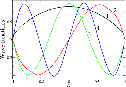
Figure 1: Four lowest eigenfunctions in the infinite Cauchy well, labeled $i=1,2,3,4$. Outcome of the $10^{4}\times 10^{4}$ matrix.

Figure 2: Left panel. Comparison of the shapes of ground state functions obtained by the diagonalization of 3x3 (black dashed curve), 5x5 (red dash-dot curve) and 30x30 (blue solid curve) matrices. The shape of ground state functions for matrices more then 30x30 are identical to that for 30x30. Right panel shows the approximation of ground state wave function (for 700x700 matrix, solid curve) by the expression (40) (dashed curve). As both lines are indistinguishable in the scale of the figure, the inset depicts the modulus of the point-wise difference of respective curves

Since, in the present paper, we employ trigonometric functions as the orthonormal basis system, for low-sized matrices (27) we deal with visually distinguishable oscillations. These are gradually smoothened with the growth of the matrix size. It is instructive to compare approximate shapes of the ground state function, obtained by the diagonalization of different-sized matrices. The left panel of Fig. 2 reports the pertinent shapes in case of $3\times 3$, $5\times 5$ and $30\times 30$ matrices. We note that the qualitative features of the ground state function approximants are practically the same for matrices of sizes exceeding $30\times 30$.

In Ref. zg an analytic approximation of the ground state function of $|\Delta|^{1/2}_{D}$ has been proposed in the form

$$\psi_{1}(x)=\psi_{g.s.}(x)=0.921749\sqrt{(1-x^{2})\cos\alpha x},\ \alpha=\frac{1443\pi}{4096}.$$ (40)

In the right panel of Fig. 2 we compare the ground state function (40) with that obtained by the diagonalization of $700\times 700$ matrix (which turns out to be close to that obtained by means of the $30\times 30$ matrix, see Fig. LABEL:fig5 below). It is seen that both functions are indistinguishable within the scale of the figure. The inset in Fig. 2 depicts the modulus of the point-wise difference of these functions. Interestingly, although the approximation is non monotonous (the difference oscillates), in a large portion of f the interval $-1\leq x\leq 1$ the difference does not exceed $0.005$.

IV.4 Eigenvalues of $|\Delta|^{1/2}_{D}$.

If compared with the previous methods of solution KKMS ; K and ZG ; zg , our spectral approach seems to be particularly powerful if one is interested in the eigenvalues of $|\Delta|^{1/2}_{D}$. In fact, we are able to generate an arbitrary number of eigenvalues, with a very high accuracy. In Table III we compare several (first 20 and a couple of larger) lowest eigenvalues of $|\Delta|^{1/2}_{D}$ and answer how much actually the ”rough” approximate formula $n\pi/2-\pi/8$ deviates from computed $E_{n}$s. That is motivated by the upper bound formula, K ; KKMS (in our notation and for the Cauchy stability index $\alpha=1$), whose right-hand-side drops down to $0$ with $n\rightarrow\infty$: $|E_{n}-\frac{n\pi}{2}+\frac{\pi}{8}|<\frac{1}{n}$.

$n$	$E_{n,5000x5000}$	$\frac{n\pi}{2}-\frac{\pi}{8}$	Relative error, %	Data from KKMS
1	1.157791	1.178097	1.75	1.157773
2	2.754795	2.748894	0.21	2.754754
3	4.316864	4.319690	0.06	4.316801
4	5.892233	5.890486	0.03	5.892147
5	7.460284	7.461283	0.013	7.460175
6	9.032984	9.032079	0.01	9.032852
7	10.602447	10.602875	0.004	10.602293
8	12.174295	12.173672	0.0051	12.174118
9	13.744308	13.744468	0.0012	13.744109
10	15.315777	15.315264	0.0033	15.315554
11	16.886062	16.886061	5.9$\cdot 10^{-8}$	*
12	18.457329	18.456857	0.0026	*
13	20.027767	20.027653	0.00057	*
14	21.598914	21.598449	0.0021	*
15	23.169448	23.169246	0.00087	*
16	24.740517	24.740042	0.0019	*
17	26.311115	26.310838	0.0011	*
18	27.882131	27.881635	0.0018	*
19	29.452773	29.452431	0.0012	*
20	31.023751	31.023227	0.0016	*
30	46.731898	46.731191	0.0015	*
50	78.148251	78.147117	0.0015	*
100	156.689159	156.686934	0.0014	*

Table 3: Several lowest eigenvalues of the $5000\times 5000$ matrix (27) are presented. For comparison the approximate formula $n\pi/2-\pi/8$ is depicted together with the relative error $|E_{n}-(n\pi/2-\pi/8)|/E_{n}$. Independently obtained spectral data (formula 1.11 in KKMS ) are displayed as well.

It is seen from the Table III that although the asymptotic formula delivers pretty good approximation to the desirable eigenvalues, the relative error never (except for $n=11$) falls below $10^{-3}$ % as the label number $n$ grows. We have actually traced this statement up to $n=500$. Moreover, the relative error, as it is seen from the Table III, oscillates around $10^{-3}$ %, which means that beginning with $n\approx 8$ the expression $n\pi/2-\pi/8$ contributes 5 significant digits of the ”true” asymptotic answer.

Technical comment: We note here that to diagonalize large matrices ($30\times 30$ and larger) we use the Fortran program, based on the LAPACK package. All integrations involved in the evaluation of $\gamma_{ki}$ and $\eta_{ki}$ have been performed numerically.

V Conclusions

In the present paper we have elaborated a novel, independent from previous proposals, method of an approximate solution of the spectral problem of the infinite Cauchy well. Our method is based on the reduction of the initial spectral problem for the operator $-|\Delta|^{1/2}$ to the Fredholm-type integral equation with the hypersingular kernel. This equation, in turn, can be solved by means of the (Fourier series) expansion with respect the complete set of orthogonal functions on the interval $-1\leq x\leq 1$ (trigonometric functions which are eigenfunctions of the Laplacian).

The adopted (Fourier series) expansion method transforms the integral eigenevalue problem (6) to the eigenvalue problem for an infinite matrix. We solve the approximate eigenvalue problems for finite  matrices, of the gradually increasing size. With the growth of the matrix size, new higher eigenvalues are generated, while lower eigenvalues becomes more and more accurate. We demonstrate that the lowest eigenfunctions can be approximately inferred by means of the diagonalization of relatively small matrices, like e.g. $30\times 30$. We have noticed that the diagonal elements of an approximating (finite) matrix give already good approximations for the eigenvalues, see Table I. To obtain the eigenvalues with $6$ significant digits the diagonalization of matrices of the size $10000\times 10000$ of more is necessary.

The method appears to be a particularly powerful tool to compute the eigenvalues. It can be generalized to other fractional (Lévy stable) operators, like e.g. $-|\Delta|_{D}^{\mu/2}$, $\mu\in(0,2)$.

References

- (1) P. Garbaczewski and V. Stephanovich, Lévy flights and nonlocal quantum dynamics, J. Math. Phys. 54, (2013) 072103.
- (2) M. Żaba and P. Garbaczewski, Solving fractional Schrödinger-type spectral problems: Cauchy oscillator and Cauchy well J. Math. Phys. 55, (2014) 092103.
- (3) P. Garbaczewski and M. Żaba, Nonlocal random motions and the trapping problem, Acta Phys. Pol. B 46, 231, (2015).
- (4) M. Żaba and P. Garbaczewski, Nonlocally-induced (fractional) bound states: Shape analysis in the infinite Cauchy well, J. Matth. Phys., 56, 123502, (2015).
- (5) P. Garbaczewski and R. Olkiewicz, Cauchy noise and affiliated stochastic processes, J. Math. Phys. 40, 1057, (1999).
- (6) A. Zoia, A. Rosso and M. Kardar, Fractional Laplacian in a bounded domain, Phys. Rev. E 76, 021116,(2007).
- (7) R. K. Getoor, First passage times for symmetric stable processes in space, Trans. Amer. Math. Soc. 101, 75, (1961).
- (8) P. Garbaczewski and W. Karwowski, Am. J. Phys., Impenetrable barriers and canonical quantization, 72, 924, (2004)
- (9) M. Belloni and R. W. Robinett, The infinite well and Dirac delta function potentials as pedagogical, mathematical and physical models in quantum mechanics, Physics Reports, 540 , 25, (2014).
- (10) M. Kwaśnicki, Ten equivalent definitions of the fractional Laplace operator, arXiv:1507.07356 [math.AP]
- (11) M. Riesz, L’integrale de Riemann-Liouville et le probléme de Cauchy, Acta Math. 81, 1-223, (1949).
- (12) J. Hadamard, Lectures on Cauchy’s Problem in Linear Partial Differential Equations, Dover, NY, 1952.
- (13) M. Kwaśnicki, Eigenvalues of the fractional Laplace operator in the interval, J. Funct. Anal. 262, 2379, (2012).
- (14) T. Kulczycki, M. Kwaśnicki, J. Małecki, A. Stós, Spectral properties of the Cauchy process on half-line and interval, Proc. London. Math. Soc. 101, 589-622, (2010).
- (15) B. Dyda, Fractional Hardy inequality with a remainder term, Colloquium Math. 122, (1), 59, (2011).
- (16) P. Garbaczewski and M. Żaba, Nonlocally induced (quasirelativistic) bound states: Harmonic confinement and the finite well, Acta Phys. Pol. B 46, 949, (2015).
- (17) E. M. Stein, Singular Integrals and Differentiability Properties of Functions, (Princeton University Press, Princeton, 1970).
- (18) A. C. Kaya and F. Erdogan, On the solution of integral equations with strongly singular kernels, Quaterly of Applied Mathematics, 45, 105, (1987)
- (19) G. Monegato,Numerical evaluation of hypersingular integrals, J. Comput. Appl. Math., 50, 9, (1994).
- (20) W. T. Ang, Hypersingular Integral Equations in Fracture Analysis, Woodhead Publ., Cambridge, 2013.
- (21) Y.-S. Chan, A. C. Fannjiang and G. H. Paulino, Integral Equations with Hypersingular Kernels-Theory and Applications to Fracture Mechanics, Int. J. of Eng. Sci., 41, 683, (2003).
- (22) J. de Klerk, Cauchy principal value and hypersingular integrals, Web notes, 2011 (available through http://www.nwu.ac.za/sites/www.nwu.ac.za/files/files/…/hipersinintegrale.pdf).
- (23) A.D. Polyanin and A.V. Manzhirov, Handbook of Integral Equations, Boca Raton-London: Chapman & Hall/CRC Press, 2008.
- (24) N. Laskin, Fractals and quantum mechanics, Chaos, 10, 780, (2000).
- (25) M. Jeng et al., On the nonlocality of the fractional Schrödinger equation, J. Math. Phys. 51, 062102 (2010).
- (26) Y. Luchko, Fractional Schrödinger equation for a particle moving in a potential well, J. Math. Phys. 54, 012111, (2013).
- (27) S. Bayin, On the consistency of solutions of the space fractional Schrödinger equation, J. Math. Phys. 53, 042105, (2012).
- (28) S. Bayin, Consistency problem of the solutions of the fractional Schrödinger equation, J. Math. Phys. 54, 092101, (2013).
- (29) A. Iomin, Lévy flights in a box, Chaos, Solitons and Fractals, 71, 73, (2015).
- (30) I.S. Gradshteyn and I.M. Ryzhik, Table of Integrals, Series, and Products, Eighth Edition by Daniel Zwillinger and Victor Moll, (2014).
- (31) Handbook of Special Functions, Eds. M. Abramowitz and I.A. Stegun, National Bureau of Standards, NY, 1964.