Directional spontaneous emission and lateral Casimir-Polder force on an atom close to a nanofiber

Abstract

We study the spontaneous emission of an excited atom close to an optical nanofiber and the resulting scattering forces. For a suitably chosen orientation of the atomic dipole, the spontaneous emission pattern becomes asymmetric and a resonant Casimir–Polder force parallel to the fiber axis arises. For a simple model case, we show that the such a lateral force is due to the interaction of the circularly oscillating atomic dipole moment with its image inside the material. With the Casimir–Polder energy being constant in the lateral direction, the predicted lateral force does not derive from a potential in the usual way. Our results have implications for optical force measurements on a substrate as well as for laser cooling of atoms in nanophotonic traps.

Electromagnetic fields close to a surface and their interaction with particles are of fundamental interest. Research in this area covers, e.g., dispersive interactions such as Casimir and Casimir–Polder (CP) forces Buhmann (2012), as well as forces that arise from the scattering of external light fields. Recently, optical forces which act perpendicularly to the propagation direction of an excitation light field attracted increasing interest Wang and Chan (2014). In particular, it has been predicted that evanescent fields exert lateral forces and torques on Mie particles Bliokh et al. (2014). Even stronger lateral forces are expected for chiral particles in evanescent fields Hayat et al. (2014).

Recent experimental research on emitters close to surfaces have revealed that suitably excited particles can be used to realize strongly directional excitation of guided modes Lin et al. (2013); Rodriguez-Fortuno et al. (2013); Luxmoore et al. (2013); Neugebauer et al. (2014); Mitsch et al. (2014); Petersen et al. (2014); le Feber et al. (2015); Söllner et al. (2014). For example, when a gold nanoparticle on the surface of an optical nanofiber scatters the light of an external circularly polarized laser beam, the coupling into counter-propagating guided modes of the nanofiber can exceed a ratio of 40:1 Petersen et al. (2014). Such an asymmetric scattering is independent of the excitation process and is only governed by the polarization of the emitted light. The conservation of total momentum in the system in conjunction with the asymmetric emission suggests the existence of a force on the scatterer that is parallel to the waveguide axis. However, the coupling to radiative modes has to be taken into account as well Xi et al. (2013). The search for such a scattering force is within reach of current cold atom experiments, in which asymmetric excitation of guided modes has already been observed Mitsch et al. (2014).

Lateral forces have also been discussed within the context of dispersion interactions where they arise even in the absence of external fields. Lateral CP forces are typically achieved by breaking the translational invariance of the surface via periodic corrugations Dalvit et al. (2008); Döbrich et al. (2008); Messina et al. (2009); Contreras-Reyes et al. (2010) or disorder Moreno et al. (2010). Moreover, lateral Casimir forces between two periodically structured surfaces have been proposed Rodrigues et al. (2006); Lambrecht and Marachevsky (2008); Chiu et al. (2009) and measured Chen et al. (2002), and have been put forward as a means to realize contactless force transmission Ashourvan et al. (2007).

Here, we propose to exploit the directional spontaneous emission by an atom near a nanofiber to realize a translationally invariant lateral CP force. The envisioned physical situation is illustrated in Fig. 1(a) and an illustration of an emission pattern is shown in Fig. 1(b). A cesium atom is located at a position $\bm{r}_{\!A}=x_{\!A}\hat{\bm{x}}$ at a distance $d_{\!A}=x_{\!A}-R$ from the surface of a fused-silica fiber of radius $R=250\,\mathrm{nm}$. The atom is initially prepared in an excited state $|1\rangle\equiv|6{}^{2}\mathrm{P}_{3/2},F^{\prime}\!=\!5,M^{\prime}_{F}\!=\!5\rangle$ . Here, the $y$ coordinate axis is chosen as the quantization axis. The only available decay channel is to the ground state $|0\rangle\equiv|6{}^{2}\mathrm{S}_{1/2},F\!=\!4,M_{F}\!=\!4\rangle$, such that the decay of the atom leads to the emission of a $\sigma^{+}$-polarized photon. The transition has a free-space wavelength of $\lambda_{10}=852\,\mathrm{nm}$, and corresponding wavenumber $k_{10}=2\pi/\lambda_{10}$ and frequency $\omega_{10}=ck_{10}$. The transition dipole matrix element is $\bm{d}_{10}=1.9\times 10^{-29}\,\mathrm{Cm}\times(\mathrm{i}\hat{\bm{x}}+\hat{\bm{z}})$ Steck (2010).

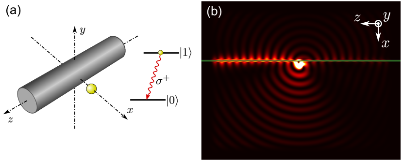
Figure 1: (a) Sketch of the situation under consideration. An atom (yellow sphere) is located at $\bm{r}_{\!A}=(x_{\!A},0,0)$, in close proximity to a nanofiber, modeled as a dielectric cylinder in free space. Calculations are performed for the cesium $D_{2}$ line optical transition at a wavelength of $\lambda_{10}=852$ nm. The atom is initially in the excited state $|1\rangle$, from where it can only decay by emitting a $\sigma^{+}$-polarized photon. The cylinder consists of silica, has a radius $R=250\,\mathrm{nm}$ and a refractive index $n=1.45$. The $y$-axis is taken as quantization axis. (b) Schematic emission pattern of a circular dipole antenna close to a waveguide obtained from a finite-difference time-domain simulation. Shown is a heat-map plot of the electric field energy density. A part of the emitted light is coupled into the waveguide (green horizontal line, width of 100 nm) and shows a strongly directional behavior, as expected Mitsch et al. (2014). The emission into radiation modes is asymmetric as well. For simplicity, the simulation is performed in two dimensions. For illustrative purposes only, we assumed a refractive index of the waveguide of $n=3>1.45$, which yields a larger asymmetry in the emission.

We use two methods to calculate the emission rates and Casimir–Polder force. The first method allows an intuitive interpretation and is based on solving the Schrödinger equation for the atom-field interaction for a suitable mode decomposition of the electric field operator Fam Le Kien et al. (2005). The second method uses the more general Green’s tensor formalism where, for example, absorption of the nanofiber is easily included.

The total spontaneous decay rate of an atom can be expressed in terms of the Green’s tensor $\mbox{{{{G}}}}(\bm{r},\bm{r}^{\prime},\omega)$ as Buhmann (2012)

$$\Gamma(\bm{r}_{\!A})=(2\mu_{0}/\hbar)\omega_{10}^{2}\bm{d}_{10}\cdot\operatorname{Im}\mbox{{{{G}}}}(\bm{r}_{\!A},\bm{r}_{\!A},\omega_{10})\cdot\bm{d}_{01}.$$ (1)

A lateral force on the atom may result from an unbalanced spontaneous emission rate into the $+z$ and $-z$ half spaces. To obtain information about the directionality of the spontaneous emission, we decompose the electric field into a set of orthonormal guided and radiation modes of the nanofiber Fam Le Kien et al. (2005). By solving the Schrödinger equation for the spontaneous emission problem See Supplemental Material at [URL will be inserted by publisher] for derivations , we obtain a total emission rate that is the sum of partial decay rates $\gamma_{fp}^{\text{(G)}}$ into guided modes, and $\gamma_{k_{z}mp}^{\text{(R)}}$ into radiation modes. Here, the index $p$ labels the polarization, $f=\pm 1$ indicates the propagation direction of the guided modes, $k_{z}$ is the projection of the wave vector of the radiation mode onto the fiber axis, and $m\in\mathbb{Z}$ is the mode order. In general, the partial decay rates depend on $\bm{r}_{\!A}$. We calculate the overall emission rates into the positive and negative half spaces as

$$\begin{split}\gamma_{\pm}^{\text{(G)}}(\bm{r}_{\!A})&=\sum_{p}\gamma^{\text{(G)}}_{f=\pm 1,p}(\bm{r}_{\!A}),\\ \gamma_{\pm}^{\text{(R)}}(\bm{r}_{\!A})&=\pm\sum_{m,p}\int_{0}^{\pm k_{10}}\!\!\mathrm{d}k_{z}\,\gamma^{\text{(R)}}_{k_{z}mp}(\bm{r}_{\!A}),\end{split}$$ (2)

where the subscript indicates into which half space the emission is directed.

Figure 2: (a) Partial decay rates $\gamma/2\pi$ into radiation and guided modes that propagate towards the $+z$ or $-z$ half space plotted as a function of the atom-surface distance $d_{\!A}$. The horizontal black dashed line indicates the free-space limit $\Gamma_{\infty}/4\pi$. (b) Directionality $\alpha$ of the total spontaneous emission. For parameters see text and Fig. 1.

The dependence of the partial decay rates on the atom-fiber distance $d_{\!A}$ is shown in Fig. 2(a). The guided modes are excited strongly asymmetrically, with emission to $+z$ being about 10 times more likely than to $-z$. This is the result of the inherent link between local polarization and propagation direction in strongly confined light fields Le Kien and Rauschenbeutel (2014) and matches the observations of a recent experiment Mitsch et al. (2014). As the intensity of the guided nanofiber modes decreases with $d_{\!A}$, so does the fraction of light that is coupled into them. The radiation modes show a complex behavior: The excitation of radiation modes that propagate into the $+z$ or $-z$ direction is, in general, also asymmetric. Moreover, the emission rates into these modes show characteristic Drexhage-type oscillations Drexhage (1970). Remarkably, depending on the radial distance of the emitter to the nanofiber surface, either the radiation modes that propagate into the $+z$ or into the $-z$ direction are excited more strongly. The amplitude of the oscillatory behavior decreases with increasing emitter-surface distance. The radiative emission into the $\pm z$ half-space is symmetric for emitters far away from the nanofiber, i.e. for ($d_{\!A}\gg\lambda_{10}$). In this limit, the total emission rate of the atom approaches the free-space value of $\Gamma_{\infty}/(2\pi)=5.234$ MHz Steck (2010).

For an atom in the proximity of the nanofiber, the combined emission rates into the $\pm z$ half space are in general not equal. The asymmetric emission should give rise to a force on the atom parallel to the fiber axis. We quantify the asymmetry by introducing a directionality parameter $\alpha$, which is a sum over all partial decay rates weighted by the projection of the respective wave vector onto the fiber axis. We denote the positive propagation constant of the guided modes at frequency $\omega_{10}$ by $\beta_{10}$. The weights are then $f\beta_{10}/k_{10}$ for guided modes and $k_{z}/k_{10}$ for radiation modes. Finally, we make $\alpha$ dimensionless by normalizing to the total emission rate,

$$\alpha(\bm{r}_{\!A})=\frac{1}{\Gamma(\bm{r}_{\!A})}\bigg{(}\sum_{f,p}\frac{f\beta_{10}}{k_{10}}\gamma_{fp}^{\text{(G)}}(\bm{r}_{\!A})\\ +\sum_{m,p}\int_{-k_{10}}^{k_{10}}\!\!\mathrm{d}k_{z}\,\frac{k_{z}}{k_{10}}\gamma_{k_{z}mp}^{\text{(R)}}(\bm{r}_{\!A})\bigg{)}.$$ (3)

Figure 2(b) shows the directionality $\alpha$ as function of $d_{\!A}$. An oscillatory, asymmetric emission is clearly visible. At the surface, the directionality reaches more than 20 %. The directionality is independent of the magnitude of the dipole moment. However, it strongly depends on the polarization of the emitted light: For the emission of a $\sigma^{-}$ instead of a $\sigma^{+}$-polarized photon, the directionality changes sign and, thus, can be controlled via the internal state of the atom. The emission is symmetric for the emission of $\pi$-polarized light.

The described directional emission in conjunction with the conservation of total momentum in the system implies a lateral force on the atom that points towards the direction of stronger emission. This force can be viewed as a Casimir–Polder force on an atom at position $\bm{r}_{\!A}$. It is given by the ensemble-averaged Lorentz force Buhmann et al. (2004) $\bm{F}=\bm{\nabla}\bigl{\langle}\hat{\bm{d}}\cdot\hat{\bm{E}}(\bm{r})\bigr{\rangle}\big{|}_{\bm{r}=\bm{r}_{\!A}}$ of the quantized vacuum electric field $\hat{\bm{E}}$ acting on the atomic dipole moment $\hat{\bm{d}}$. After solving the coupled atom-field dynamics and evaluating the averages over the atomic and field states, one finds for an atom initially in an energy eigenstate $|n\rangle$ a force $\bm{F}_{n}(\bm{r}_{\!A})=\bm{F}_{n}^{\mathrm{nres}}(\bm{r}_{\!A})+\bm{F}_{n}^{\mathrm{res}}(\bm{r}_{\!A})$. The Green’s tensor can be decomposed into a vacuum part $\mbox{{{{G}}}}^{(0)}$ and a part $\mbox{{{{G}}}}^{(1)}$ associated to the scattering of the electric field from the nanofiber. Only the latter can give rise to a force. The non-resonant part of the force, $\bm{F}_{n}^{\text{nres}}(\bm{r}_{\!A})$, is proportional to the gradient of the symmetric part of $\mbox{{{{G}}}}^{(1)}$. The resonant part, $\bm{F}_{n}^{\text{res}}(\bm{r}_{\!A})$, contains the gradient of the Hermitian part of $\mbox{{{{G}}}}^{(1)}$ See Supplemental Material at [URL will be inserted by publisher] for derivations .

When the atomic state $|n\rangle$ and the Hamiltonian are time-reversal symmetric, the dipole-matrix elements can be chosen real. In such cases, the gradient $\bm{\nabla}$ can be replaced with a total derivative $\bm{\nabla}_{\bm{r}_{\!A}}$, showing that no forces exist in a direction in which the system is translationally invariant. We require an atom in an eigenstate that is not time-reversal symmetric, such that complex dipole-matrix elements can give rise to a lateral force.

To see whether such forces can exist, let us consider an infinitely long cylinder. Its Green’s tensor is translationally invariant along the cylinder axis $z$, so that $(\partial/\partial z)\mbox{{{{G}}}}^{(1)}(\bm{r},\bm{r}^{\prime},\omega)=-(\partial/\partial z^{\prime})\mbox{{{{G}}}}^{(1)}(\bm{r},\bm{r}^{\prime},\omega)$ holds. Combining this with the Onsager reciprocity relation $\mbox{{{{G}}}}^{(1)}(\bm{r},\bm{r}^{\prime},\omega)=\mbox{{{{G}}}}^{(1){\operatorname{T}}}(\bm{r}^{\prime},\bm{r},\omega)$, we find that the derivative with respect to $z$ of the scattering part of the Green’s tensor is anti-symmetric. This immediately shows that for a ground-state atom with its purely off-resonant CP force a lateral force cannot exist. Such a lateral force is also forbidden by energy conservation: If it existed, one could use it to accelerate a ground-state atom along the fiber and, thus, gain kinetic energy while leaving the internal energy of the atom and that of the environment unchanged.

A lateral force can thus only arise due to the resonant component which is associated with the recoil of the atom when undergoing an optical transition between two states. These forces are fueled by the atom’s internal energy. Using the anti-symmetry mentioned above, the lateral force is given by

$$F_{n,z}^{\text{res}}(\bm{r}_{\!A})=2\mathrm{i}\mu_{0}\sum_{k<n}\omega_{nk}^{2}\\ \times\bm{d}_{nk}\cdot\,\frac{\partial}{\partial z}\operatorname{Im}\mbox{{{{G}}}}^{(1)}(\bm{r},\bm{r}_{\!A},\omega_{nk})\cdot\bm{d}_{kn}\big{|}_{\bm{r}=\bm{r}_{\!A}}.$$ (4)

Being proportional to $\operatorname{Im}\mbox{{{{G}}}}$, it is associated with the out-of-phase interaction of the electric-dipole oscillations with the reflected electric field. By contrast, the normal resonant CP force depends on the real part of the Green’s tensor.

For the numerical evaluation of the force, we insert the scattering part of the Green’s tensor

$$\mbox{{{{G}}}}^{(1)}(\bm{r},\bm{r}^{\prime},\omega)=\frac{\mathrm{i}}{8\pi}\int_{-\infty}^{\infty}\mathrm{d}k_{z}\sum_{m=0}^{\infty}\sum_{p,p^{\prime}=T\!E,T\!M}\\ \times\frac{2-\delta_{0m}}{k_{\rho}^{2}}r_{pp^{\prime}}\bm{a}_{k_{z}mp}(\bm{r})\otimes\bm{a}_{-k_{z}mp^{\prime}}(\bm{r}^{\prime})$$ (5)

($\delta_{ij}$: Kronecker symbol) of a cylinder, which is given in terms of cylindrical vector wave functions $\bm{a}_{k_{z}mp}$ and the respective reflection coefficients $r_{pp^{\prime}}$ Li et al. (2000) with the dispersion relation $\omega^{2}/c^{2}=k^{2}=k_{z}^{2}+k_{\rho}^{2}$. Assuming a cesium atom in the excited state $|n\rangle=|1\rangle$ with a single downward transition to the ground state $|k\rangle=|0\rangle$, and using the complex refractive index $1.45+\mathrm{i}2.05\times 10^{-7}$ of fused silica Kitamura et al. (2007) at the transition frequency $\omega_{10}$, we can numerically evaluate the lateral force (4). We compare this to a calculation based on the solution of the Schrödinger equation where the expression for the lateral force based on the guided and radiation modes of the nanofiber is See Supplemental Material at [URL will be inserted by publisher] for derivations

$$F_{1,z}(\bm{r}_{\!A})=-\hbar\bigg{(}\sum_{f,p}f\beta_{10}\gamma_{fp}^{\text{(G)}}(\bm{r}_{\!A})\\ +\sum_{m,p}\int_{-k_{10}}^{k_{10}}\!\mathrm{d}k_{z}\,k_{z}\gamma_{k_{z}mp}^{\text{(R)}}(\bm{r}_{\!A})\bigg{)}.$$ (6)

Here, the recoil nature of the force becomes evident, as the summation is over partial decay rates into guided and radiation modes multiplied by the photon momentum of the respective mode.

The result of the numerical evaluation of Eqs. (4) and (6) is displayed in Fig. 3(a). One observes an oscillating force with a distance dependence similar to the directionality parameter shown in Fig. 2(b) but which, as expected from momentum conservation, points into the direction opposite to the dominant emission. The lateral force is an illustration of the subtle differences between Casimir–Polder force and potential Buhmann et al. (2004): It exists in spite of the $z$-independence of the Casimir–Polder potential and hence cannot be derived from the latter.

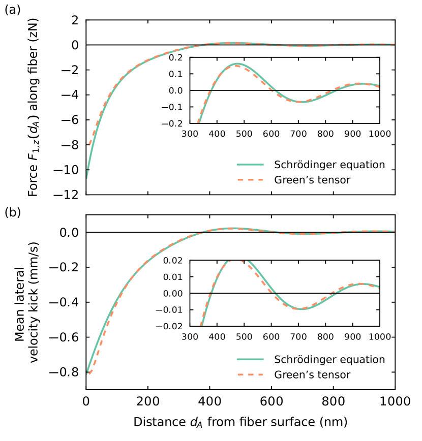
Figure 3: (a) Lateral Casimir-Polder force $F_{1,z}(d_{A},t=0)$ on an excited cesium atom at distance as $d_{\!A}$ from the nanofiber surface. (b) Mean lateral velocity increase per emitted photon. Force and velocity have been calculated using a method based on the solution of the Schrödinger equation, and using the Green’s tensor. Insets show magnifications for distances above 300 nm. We attribute the small deviation between the two methods to numerical artifacts. For parameters see text.

Recall that the lateral force is a result of the decay of the atom to its ground state and the associated emission of a photon. Thus, the time dependence of the ensemble-averaged force is given by $F_{1,z}(\bm{r}_{\!A},t)=\mathrm{e}^{-\Gamma t}F_{1,z}(\bm{r}_{\!A})$. We thus obtain an average momentum kick per emitted photon of

$$\Delta\langle p_{z}\rangle=F_{1,z}^{\mathrm{res}}(\bm{r}_{\!A})/\Gamma(\bm{r}_{\!A})=-\alpha\hbar k_{10},$$ (7)

where $\alpha$ is the directionality defined in Eq. (3). Figure 3(b) shows the velocity gained per photon, which can reach values of up to $0.8\mbox{ mm/s}$ in our situation.

The agreement between both methods provides some understanding of the mechanism that underlies the lateral force. Note, however, that the Green’s tensor approach is more general and also allows for the investigation of situations where the fiber shows substantial losses that prevent the introduction of orthonormal modes. Indeed, an artificial increase of the imaginary part of the refractive index by five orders of magnitude to $2\times 10^{-2}$ results in a 50 % larger lateral force, which is likely to be driven by the increased nonradiative decay that is automatically captured in the Green’s tensor formalism.

To gain some further intuition into the lateral force, we consider the simpler case of an atom in front of a semi-infinite half space. In this case, the scattering Green tensor takes the form

$$\mbox{{{{G}}}}^{(1)}(\bm{r},\bm{r}^{\prime},\omega)=\frac{\mathrm{i}}{8\pi^{2}}\,\int\frac{\mathrm{d}^{2}k^{\parallel}}{k_{x}}\,\mathrm{e}^{\mathrm{i}\bm{k}^{\parallel}\cdot(\bm{r}-\bm{r}^{\prime})+\mathrm{i}k_{x}(z+z^{\prime})}\\ \times\sum_{p=T\!E,T\!M}r_{p}\bm{e}_{\sigma+}\bm{e}_{\sigma-}$$ (8)

with polarization unit vectors $\bm{e}_{\sigma\pm}$, Fresnel reflection coefficients $r_{p}$ and the dispersion relation $\omega^{2}/c^{2}=k^{2}=k_{x}^{2}+{(k^{\parallel})}^{2}$. Substitution into Eq. (4) then leads to a simple expression for the lateral Casimir–Polder force in the retarded limit $d_{A}\gg\lambda_{10}$: in this case, the wave-vector integral is dominated by the stationary-phase point at $k^{\parallel}=0$ and we find for weak absorption:

$$F_{1,z}^{\mathrm{res}}(d_{\!A})=\frac{\operatorname{Im}(d_{01,z}d_{10,x})\omega_{10}^{2}}{8\varepsilon_{0}c^{2}d_{A}^{2}}\sin(2d_{\!A}k_{10})\,r_{p}$$ (9)

with $r_{p}=[n(\omega_{10})-1]/[n(\omega_{10})+1]$. One sees that the lateral force is due to the interaction of the atom with its image dipole behind the surface of the half space. Also for this model case, we observe Drexhage-type oscillations.

In summary, we have theoretically described a translationally invariant lateral scattering force which arises from asymmetric spontaneous emission of a circular dipole emitter that is in close proximity to an optical nanofiber. In contrast to all lateral forces previously studied in Casimir and Casimir–Polder physics, the force does not rely on a corrugation of the material surface. Moreover, the magnitude and sign of the force depend on the polarization of the emitted light and thus can be controlled, e.g., by the quantum state of an atomic emitter. The described lateral force is generic in the sense that it prevails also in other geometries, e.g. for circular emitters above a plane surface. In contrast to the forces on Mie particles proposed in Bliokh et al. (2014), our lateral force does not rely on a higher-order interaction between electric- and magnetic-induced dipoles.

In optical force measurements on particles on a substrate Neuman and Block (2004), this effect will influence measurement outcomes as soon as scattering becomes relevant. Moreover, we expect the lateral force to enrich the dynamics of optically driven self-organization of atomic ensembles close to waveguides Chang et al. (2013); Holzmann et al. (2014). In order to tune the force, the atom can be coupled to, e.g., a whispering-gallery mode optical resonator Junge et al. (2013); Shomroni et al. (2014), thereby changing the relative share of emission into guided and radiative modes. Lateral forces as described here will also influence laser cooling of atoms close to surfaces Hammes et al. (2003); Stehle et al. (2014) and nanophotonic structures Vetsch et al. (2012); Thompson et al. (2013); Goban et al. (2014). The study of lateral scattering forces might be extended to thermal Casimir–Polder forces or to other geometries, e.g., an atom above a sphere where the lateral position is coupled to the atom-surface distance.

We thank F. Ciccarello, F. Intravaia, Fam Le Kien, A. Rauschenbeutel, C. Sayrin, and J. Volz for helpful comments and discussions. Financial support by the DFG (grant no. SCHE 612/2-1) is gratefully acknowledged. S. Y. B. gratefully acknowledges support by the DFG (grant BU 1803/3-1) and the Freiburg Institute for Advanced Studies.

Appendix A Partial emission rates

In this Supplement we present the calculation based on the solution of the Schrödinger equation for a cesium atom close to the nanofiber. The atom is initially in the hyperfine state $\left|1\right\rangle=\left|F^{\prime}=5,M_{F}^{\prime}=5\right\rangle$ of the $6P_{3/2}$ manifold. The only available decay channel is to the hyperfine ground state $\left|0\right\rangle=\left|F=4,M_{F}=4\right\rangle$ through the emission of a $\sigma^{+}$-polarized photon at frequency $\omega_{10}$, and we can treat the atom as an effective two-level system. In the interaction picture, the atomic dipole operator is given by

$$\hat{\bm{d}}=\bm{d}_{01}\left|0\right\rangle\!\!\left\langle{1}\right|e^{-\mathrm{i}\omega_{10}t}+\bm{d}_{10}\left|1\right\rangle\!\!\left\langle{0}\right|e^{\mathrm{i}\omega_{10}t},$$ (10)

where $\bm{d}_{01}=\bm{d}_{10}^{*}$ is the corresponding dipole matrix element. We follow Fam Le Kien et al. (2005) and decompose the electric field into contributions from guided and radiation modes, neglecting material absorption. For the guided modes we assume that the single-mode condition is satisfied for a finite bandwidth around $\omega_{10}$. In cylindrical coordinates $\bm{r}=(r,\phi,z)$, the positive-frequency part of the guided-mode field operator in the interaction picture can be written as

$$\hat{\bm{E}}_{G}^{(+)}(\bm{r})=\mathrm{i}\sum_{f,p}\int_{0}^{\infty}\!\!\mathrm{d}\omega\sqrt{\frac{\hbar\omega\beta^{\prime}}{4\pi\epsilon_{0}}}\\ \times\hat{a}_{\omega fp}\bm{e}_{\omega fp}(r)e^{-\mathrm{i}(\omega t-f\beta z-p\phi)}.$$ (11)

Here, $\beta$ is the propagation constant of the guided mode, $\beta^{\prime}=\mathrm{d}\beta/\mathrm{d}\omega$, $\hat{a}_{\omega fp}$ is the annihilation operator and $\bm{e}_{\omega fp}$ is the profile function of the guided mode. The indices $f=\pm 1$ and $p=\pm 1$ indicate the propagation direction and the handedness of the quasi-circular polarization, respectively Fam Le Kien et al. (2005). Similarly, for the radiation modes

$$\hat{\bm{E}}_{R}^{(+)}(\bm{r})=\mathrm{i}\sum_{m,p}\int_{0}^{\infty}\!\!\mathrm{d}\omega\int_{-\omega/c}^{\omega/c}\!\!\mathrm{d}k_{z}\sqrt{\frac{\hbar\omega}{4\pi\epsilon_{0}}}\\ \times\hat{a}_{\omega k_{z}mp}\bm{e}_{\omega k_{z}mp}(r)e^{-\mathrm{i}(\omega t-k_{z}z-m\phi)},$$ (12)

where $k_{z}$ is the projection of the wave vector onto the fiber axis, $m\in\mathbb{Z}$ is the mode order, and $p$ is the mode polarization.

Let $\bm{r}_{A}$ denote the position of the atom. The Hamiltonian for the atom-field interaction in the dipole and rotating-wave approximations is given by

$$\begin{split}\hat{H}_{\text{int}}&=-\hat{\bm{d}}\cdot\hat{\bm{E}}(\bm{r}_{A})\\ &=-\mathrm{i}\hbar\sum_{f,p}\int_{0}^{\infty}\!\!\mathrm{d}\omega\,G_{\omega fp}(\bm{r}_{A})\left|1\right\rangle\!\!\left\langle{0}\right|\hat{a}_{\omega fp}e^{-\mathrm{i}(\omega-\omega_{10})t}\\ &\quad-\mathrm{i}\hbar\sum_{m,p}\int_{0}^{\infty}\!\!\mathrm{d}\omega\int_{-\omega/c}^{\omega/c}\!\!\mathrm{d}k_{z}\,G_{\omega k_{z}mp}(\bm{r}_{A})\\ &\qquad\times\left|1\right\rangle\!\!\left\langle{0}\right|\hat{a}_{\omega k_{z}mp}e^{-\mathrm{i}(\omega-\omega_{10})t}+\text{H. c.}\end{split}$$ (13)

We have introduced the coefficients $G_{\omega fp}(\bm{r})$ and $G_{\omega k_{z}mp}(\bm{r})$ which characterize the coupling of the atomic transition to a specific guided or radiation mode, respectively. These coefficients are given by

$$\begin{split}G_{\omega fp}(\bm{r})&=\sqrt{\frac{\omega\beta^{\prime}}{4\pi\epsilon_{0}\hbar}}\bm{d}_{10}\cdot\bm{e}_{\omega fp}(r)\,e^{\mathrm{i}(f\beta z+p\phi)},\\ G_{\omega k_{z}mp}(\bm{r})&=\sqrt{\frac{\omega}{4\pi\epsilon_{0}\hbar}}\bm{d}_{10}\cdot\bm{e}_{\omega k_{z}fp}(r)\,e^{\mathrm{i}(k_{z}z+m\phi)}.\end{split}$$ (14)

For the combined atom-field state, we restrict the Hilbert space to a single excitation. In the following, the first element of the state vector indicates the state of the atom and the second element that of the field. Then, the atom-field state at any time can be written as

$$\left|\psi(t)\right\rangle=c_{1}(t)\left|1,0\right\rangle+\sum_{f,p}\int_{0}^{\infty}\!\!\mathrm{d}\omega\,c_{\omega fp}(t)\left|0,1_{\omega fp}\right\rangle$$

$$+\sum_{m,p}\int_{0}^{\infty}\!\!\mathrm{d}\omega\int_{-\omega/c}^{\omega/c}\!\!\mathrm{d}k_{z}\,c_{\omega k_{z}mp}\left|0,1_{\omega k_{z}mp}\right\rangle.$$ (15)

We obtain expressions for the time-dependent coefficients $c(t)$ by inserting into the Schrödinger equation and following a standard Wigner-Weisskopf treatment. First, we formally integrate the differential equations for the guided and radiation mode coefficients. Applying a Markov approximation, we replace $c_{1}(t^{\prime})$ by $c_{1}(t)$ in the resulting expressions and obtain

$$\begin{split}c_{\omega fp}(t)&=c_{1}(t)\,G_{\omega fp}^{*}(\bm{r}_{A})\int_{0}^{t}\!\!\mathrm{d}t^{\prime}e^{\mathrm{i}(\omega-\omega_{10})t^{\prime}},\\ c_{\omega k_{z}mp}(t)&=c_{1}(t)\,G_{\omega k_{z}mp}^{*}(\bm{r}_{A})\int_{0}^{t}\!\!\mathrm{d}t^{\prime}e^{\mathrm{i}(\omega-\omega_{10})t^{\prime}}.\\ \end{split}$$ (16)

These are inserted into the differential equation for $c_{1}(t)$, where we let the upper limits of the time integrals tend to infinity. Solving the integrals, we further neglect the term corresponding to a vacuum frequency shift and obtain a simple exponential decay, $c_{1}(t)=e^{-\Gamma t/2}$ with a total, position-dependent spontaneous-emission rate $\Gamma(\bm{r}_{\!A})$ as

$$\frac{\Gamma(\bm{r}_{\!A})}{2\pi}=\sum_{f,p}\left|G_{\omega_{10}fp}(\bm{r}_{A})\right|^{2}\\ +\sum_{m,p}\int_{-k_{10}}^{k_{10}}\!\!\mathrm{d}k_{z}\,\left|G_{\omega_{10}k_{z}mp}(\bm{r}_{A})\right|^{2}.$$ (17)

We see that each guided mode has an associated partial emission rate given by

$$\begin{split}\gamma_{fp}^{\text{(G)}}(\bm{r}_{\!A})&=2\pi\left|G_{\omega_{10}fp}(\bm{r_{\!A}})\right|^{2}\\ &=\frac{\omega_{10}\beta_{10}^{\prime}}{2\epsilon_{0}\hbar}\left|\bm{d}_{10}\cdot\bm{e}_{\omega_{10}fp}(\bm{r}_{\!A})\right|^{2},\end{split}$$ (18)

and similarly for the radiation modes,

$$\begin{split}\gamma_{k_{z}mp}^{\text{(R)}}(\bm{r}_{\!A})&=2\pi\left|G_{\omega_{10}k_{z}mp}(\bm{r_{\!A}})\right|^{2}\\ &=\frac{\omega_{10}}{2\epsilon_{0}\hbar}\left|\bm{d}_{10}\cdot\bm{e}_{\omega_{10}k_{z}mp}(\bm{r}_{\!A})\right|^{2}.\end{split}$$ (19)

To study the directional dependence of the spontaneous emission, we note that the partial decay rates into each guided or radiation mode are proportional to the absolute square of the coupling coefficients (14). The propagation direction along the fiber axis for the guided modes is encoded in the parameter $f$, such that $f=+1$ corresponds to emission into the positive half space. Similarly, for the radiation modes it is encoded into the projection $k_{z}$ of the wave vector, and emission into the positive half space is represented by modes with $k_{z}>0$. Hence, the partial decay rates into the half spaces $\pm z$ for guided ($\gamma_{\pm}^{\text{(G)}}$) and radiation modes ($\gamma_{\pm}^{\text{(G)}}$) are given by

$$\begin{split}\gamma_{\pm}^{\text{(G)}}(\bm{r}_{\!A})&=\sum_{p}\gamma_{f=\pm 1,p}^{\text{(G)}}(\bm{r}_{\!A}),\\ \gamma_{\pm}^{\text{(R)}}(\bm{r}_{\!A})&=\pm\sum_{m,p}\int_{0}^{\pm k_{10}}\!\!\mathrm{d}k_{z}\,\gamma_{k_{z}mp}^{\text{(R)}}(\bm{r}_{\!A}),\\ \end{split}$$ (20)

which is Eq. (2) in the main text.

Appendix B Lorentz Force

The calculation of the Lorentz force amounts to computing the expectation value $\langle\bm{F}\rangle=\bm{\nabla}\langle\hat{\bm{d}}\cdot\hat{\bm{E}}(\bm{r})\rangle|_{\bm{r}=\bm{r}_{A}}$. We note that, in contrast to the interaction Hamiltonian (13), here the field operator is evaluated at a general position $\bm{r}$. The position of the atom is only inserted after taking the gradient.

We are only interested in the lateral part of the force, i.e., $\langle F_{z}\rangle=\frac{\partial}{\partial z}\langle\hat{\bm{d}}\cdot\hat{\bm{E}}(\bm{r})\rangle|_{\bm{r}=\bm{r}_{A}}$. To keep track of the individual contributions to the force, we label the part of the state (15) that describes excitations of the guided modes $\left|\psi_{G}\right\rangle$, and similarly for the radiation modes $\left|\psi_{R}\right\rangle$. The Lorentz force is then given by the sum of two terms, $\langle F_{z}\rangle=\langle F_{z}^{\text{(G)}}\rangle+\langle F_{z}^{\text{(R)}}\rangle$, where

$$\langle F_{z}^{\text{(M)}}\rangle=2\operatorname{Re}\left(c_{1}^{*}(t)\frac{\partial}{\partial z}V_{1,M}(\bm{r})\right)\bigg{|}_{\bm{r}=\bm{r}_{A}},$$ (21)

and $M\in\{G,R\}$. We have introduced the matrix element $V_{1,M}=\left\langle{1,0}\right|\hat{\bm{d}}^{(-)}\cdot\hat{\bm{E}}_{M}^{(+)}(\bm{r})\left|\psi_{M}\right\rangle$, where $\hat{\bm{d}}^{(-)}$ is the negative-frequency part of the dipole operator, i.e., the second term in Eq. (10).

For the guided modes, we find

$$\begin{split}V_{1,G}(\bm{r})&=-\hbar e^{-\Gamma t/2}\sum_{f,p}\int_{0}^{\infty}\mathrm{d}\omega\,G_{\omega fp}(\bm{r})G_{\omega fp}^{*}(\bm{r}_{A})\\ &\qquad\times\frac{e^{-\mathrm{i}(\omega-\omega_{10})t}-1}{\omega-\omega_{10}}\\ &\approx-A(t)e^{-\Gamma t/2}\frac{\beta_{10}^{\prime}}{4\pi\epsilon_{0}}\\ &\qquad\times\sum_{f,p}[\bm{d}_{10}\cdot\bm{e}_{\omega_{10}fp}(\bm{r})]{[\bm{d}_{10}\cdot\bm{e}_{\omega_{10}fp}(\bm{r}_{\!A})]}^{*}\\ &\qquad\qquad\times e^{\mathrm{i}[f\beta_{10}(z-z_{A})+p(\phi-\phi_{A})]},\end{split}$$ (22)

where for the approximation we have made use of the fact that the mode functions, propagation constant, and their derivatives vary slowly in a frequency interval around $\omega_{10}$, for which we expect the main contribution to the integral in (22). We hence replace them by their resonant values, such that the remaining integral is

$$\begin{split}A(t)&=\int_{0}^{\infty}\!\!\mathrm{d}\omega\,\omega\frac{e^{-\mathrm{i}(\omega-\omega_{10})t}-1}{\omega-\omega_{10}}\\ &\approx\int_{-\infty}^{\infty}\!\!\mathrm{d}\Delta\,(\omega_{10}+\Delta)\frac{e^{-\mathrm{i}\Delta t}-1}{\Delta}=-\mathrm{i}\pi\omega_{10}.\end{split}$$ (23)

In the second line, we substituted $\Delta=\omega-\omega_{10}$ and extended the lower limit of the integral from $-\omega_{10}$ to $-\infty$. Inserting (23) and (22) into (21), we find that the lateral force due to spontaneous emission into guided modes is

$$\langle F_{z}^{\text{(G)}}\rangle=-e^{-\Gamma t}\frac{\omega_{10}\beta_{10}\beta_{10}^{\prime}}{2\epsilon_{0}}\sum_{f,p}f\left|\bm{d}_{10}\cdot\bm{e}_{\omega_{10}fp}(\bm{r}_{\!A})\right|^{2}.$$ (24)

The calculation for the contribution from the radiation modes is similar. The approximation that the main contribution stems from a narrow frequency interval around the resonance allows us to set the limits of the integral over $k_{z}$ to $\pm k_{10}$ and take it out of the frequency integral. Hence,

$$V_{1,R}(\bm{r})\approx-\frac{A(t)e^{-\Gamma t/2}}{4\pi\epsilon_{0}}\sum_{m,p}\int_{-k_{10}}^{k_{10}}\!\!\mathrm{d}k_{z}e^{\mathrm{i}[k_{z}(z-z_{A})+m(\phi-\phi_{A})]}$$

$$\times[\bm{d}_{10}\cdot\bm{e}_{\omega_{10}k_{z}mp}(r)]{[\bm{d}_{10}\cdot\bm{e}_{\omega_{10}k_{z}mp}(\bm{r}_{\!A})]}^{*}$$ (25)

such that

$$\langle F_{z}^{\text{(R)}}\rangle=-e^{-\Gamma t}\frac{\omega_{10}}{2\epsilon_{0}}\sum_{m,p}\int_{-k_{10}}^{k_{10}}\!\!\mathrm{d}k_{z}\,k_{z}\left|\bm{d}_{10}\cdot\bm{e}_{\omega_{10}k_{z}mp}(\bm{r}_{\!A})\right|^{2}.$$ (26)

Finally, we note that Eqs. (24) and (26) can be rewritten in terms of the partial decay rates of Eqs. (18) and (19),

$$\begin{split}\langle F_{z}^{\text{(G)}}\rangle&=-\hbar e^{-\Gamma t}\sum_{f,p}f\beta_{10}\gamma_{fp}^{\text{(G)}}(\bm{r}_{\!A}),\\ \langle F_{z}^{\text{(R)}}\rangle&=-\hbar e^{-\Gamma t}\sum_{m,p}\int_{-k_{10}}^{k_{10}}\!\mathrm{d}k_{z}\,k_{z}\gamma_{k_{z}mp}^{\text{(R)}}(\bm{r}_{\!A}).\end{split}$$ (27)

Appendix C Resonant and non-resonant parts of the Lorentz force

In general, the Lorentz force contains contributions from resonant and non-resonant components, $\bm{F}_{n}(\bm{r}_{\!A})=\bm{F}_{n}^{\mathrm{nres}}(\bm{r}_{\!A})\rangle+\bm{F}_{n}^{\mathrm{res}}(\bm{r}_{\!A})$. We give here their full analytical expressions based on the Green’s tensor G. In particular, the non-resonant component is Buhmann et al. (2004)

$$\bm{F}_{n}^{\mathrm{nres}}(\bm{r}_{\!A})=-\frac{2\mu_{0}}{\pi}\sum_{k}\int_{0}^{\infty}\mathrm{d}\xi\,\frac{\xi^{2}\omega_{kn}}{\omega_{kn}^{2}+\xi^{2}}\\ \times\bm{\nabla}\bm{d}_{nk}\cdot\mathcal{S}\mbox{{{{G}}}}^{(1)}(\bm{r},\bm{r}_{\!A},\mathrm{i}\xi)\cdot\mathbf{d}_{kn}\big{|}_{\bm{r}=\bm{r}_{A}}~{},$$ (28)

where $\mathcal{S}\mbox{{{{G}}}}=(\mbox{{{{G}}}}+\mbox{{{{G}}}}^{\operatorname{T}})/2$ is the symmetric part of a tensor. The resonant component is given by

$$\bm{F}_{n}^{\mathrm{res}}(\bm{r}_{\!A})=2\mu_{0}\sum_{k<n}\omega_{nk}^{2}\\ \times\bm{\nabla}\bm{d}_{nk}\cdot\mathcal{H}\mbox{{{{G}}}}^{(1)}(\bm{r},\bm{r}_{\!A},\omega_{nk})\cdot\bm{d}_{kn}\big{|}_{\bm{r}=\bm{r}_{\!A}}~{},$$ (29)

where $\mathcal{H}\mbox{{{{G}}}}=(\mbox{{{{G}}}}+\mbox{{{{G}}}}^{\ast{\operatorname{T}}})/2$ is the Hermitian part. Here, $\omega_{kn}$ and $\bm{d}_{nk}$ are the frequencies and matrix elements for electric-dipole transitions of the atom and $\mbox{{{{G}}}}^{(1)}$ is the scattering part of the classical Green’s tensor for the electric field.

The directionality parameter $\alpha$ given in the main manuscript can also be expressed in terms of the Green’s tensor as

$$\alpha=\frac{-2}{k_{10}}\left[\frac{\partial}{\partial z}\operatorname{Im}G_{xz}^{(1)}\right]\bigg{[}\operatorname{Im}G_{xx}+\operatorname{Im}G_{zz}\bigg{]}^{-1}.$$ (30)

References

- Buhmann (2012) S. Y. Buhmann, Dispersion Forces I — Macroscopic Quantum Electrodynamics and Ground-State Casimir, Casimir–Polder and van der Waals Forces (Springer, 2012).
- Wang and Chan (2014) S. B. Wang and C. T. Chan, Nat. Commun. 5, 3307 (2014).
- Bliokh et al. (2014) K. Y. Bliokh, A. Y. Bekshaev, and F. Nori, Nat. Commun. 5, 3300 (2014).
- Hayat et al. (2014) A. Hayat, J. P. Balthasar Müller, and F. Capasso, (2014), arXiv:1408.2268 .
- Lin et al. (2013) J. Lin, J. P. B. Mueller, Q. Wang, G. Yuan, N. Antoniou, X.-C. Yuan, and F. Capasso, Science 340, 331 (2013).
- Rodriguez-Fortuno et al. (2013) F. J. Rodriguez-Fortuno, G. Marino, P. Ginzburg, D. O’Connor, A. Martínez, G. A. Wurtz, and A. V. Zayats, Science 340, 328 (2013).
- Luxmoore et al. (2013) I. J. Luxmoore, N. A. Wasley, A. J. Ramsay, A. C. T. Thijssen, R. Oulton, M. Hugues, A. M. Fox, and M. S. Skolnick, Appl. Phys. Lett. 103, 241102 (2013).
- Neugebauer et al. (2014) M. Neugebauer, T. Bauer, P. Banzer, and G. Leuchs, Nano Lett. 14, 2546 (2014).
- Mitsch et al. (2014) R. Mitsch, C. Sayrin, B. Albrecht, P. Schneeweiss, and A. Rauschenbeutel, Nat. Commun. 5, 5713 (2014).
- Petersen et al. (2014) J. Petersen, J. Volz, and A. Rauschenbeutel, Science 346, 67 (2014).
- le Feber et al. (2015) B. le Feber, N. Rotenberg, and L. Kuipers, Nat. Commun. 6, 6695 (2015).
- Söllner et al. (2014) I. Söllner, S. Mahmoodian, S. Lindskov Hansen, L. Midolo, A. Javadi, G. Kiršanskė, T. Pregnolato, H. El-Ella, E. Hye Lee, J. D. Song, S. Stobbe, and P. Lodahl, (2014), arXiv:1406.4295 .
- Xi et al. (2013) Z. Xi, Y. Lu, P. Yao, W. Yu, P. Wang, and H. Ming, Opt. Express 21, 30327 (2013).
- Dalvit et al. (2008) D. A. R. Dalvit, P. A. M. Neto, A. Lambrecht, and S. Reynaud, Phys. Rev. Lett. 100, 040405 (2008).
- Döbrich et al. (2008) B. Döbrich, M. DeKieviet, and H. Gies, Phys. Rev. D 78, 125022 (2008).
- Messina et al. (2009) R. Messina, D. A. R. Dalvit, P. A. M. Neto, A. Lambrecht, and S. Reynaud, Phys. Rev. A 80, 022119 (2009).
- Contreras-Reyes et al. (2010) A. M. Contreras-Reyes, R. Guérout, P. A. M. Neto, D. A. R. Dalvit, A. Lambrecht, and S. Reynaud, Phys. Rev. A 82, 052517 (2010).
- Moreno et al. (2010) G. A. Moreno, R. Messina, D. A. R. Dalvit, A. Lambrecht, P. A. M. Neto, and S. Reynaud, Phys. Rev. Lett. 105, 210401 (2010).
- Rodrigues et al. (2006) R. B. Rodrigues, P. A. M. Neto, A. Lambrecht, and S. Reynaud, Phys. Rev. Lett. 96, 100402 (2006).
- Lambrecht and Marachevsky (2008) A. Lambrecht and V. N. Marachevsky, Phys. Rev. Lett. 101, 160403 (2008).
- Chiu et al. (2009) H.-C. Chiu, G. L. Klimchitskaya, V. N. Marachevsky, V. M. Mostepanenko, and U. Mohideen, Phys. Rev. B 80, 121402 (2009).
- Chen et al. (2002) F. Chen, U. Mohideen, G. L. Klimchitskaya, and V. M. Mostepanenko, Phys. Rev. Lett. 88, 101801 (2002).
- Ashourvan et al. (2007) A. Ashourvan, M. F. Miri, and R. Golestanian, Phys. Rev. Lett. 98, 140801 (2007).
- Steck (2010) D. A. Steck, available online at http://steck.us/alkalidata (2010).
- Fam Le Kien et al. (2005) Fam Le Kien, S. Dutta Gupta, V. I. Balykin, and K. Hakuta, Phys. Rev. A 72, 032509 (2005).
- (26) See Supplemental Material at [URL will be inserted by publisher] for derivations, .
- Le Kien and Rauschenbeutel (2014) F. Le Kien and A. Rauschenbeutel, Phys. Rev. A 90, 023805 (2014).
- Drexhage (1970) K. Drexhage, J. Lumin. 1, 693 (1970).
- Buhmann et al. (2004) S. Y. Buhmann, L. Knöll, D.-G. Welsch, and H. T. Dung, Phys. Rev. A 70, 052117 (2004).
- Li et al. (2000) L.-W. Li, M.-S. Leong, T.-S. Yeo, and P.-S. Kooi, J. Electromagn. Wave. 14, 961 (2000).
- Kitamura et al. (2007) R. Kitamura, L. Pilon, and M. Jonasz, Appl. Opt. 46, 8118 (2007).
- Neuman and Block (2004) K. C. Neuman and S. M. Block, Rev. Sci. Instrum. 75, 2787 (2004).
- Chang et al. (2013) D. E. Chang, J. I. Cirac, and H. J. Kimble, Phys. Rev. Lett. 110, 113606 (2013).
- Holzmann et al. (2014) D. Holzmann, M. Sonnleitner, and H. Ritsch, Eur. Phys. J. D 68, 1 (2014).
- Junge et al. (2013) C. Junge, D. O’Shea, J. Volz, and A. Rauschenbeutel, Phys. Rev. Lett. 110, 213604 (2013).
- Shomroni et al. (2014) I. Shomroni, S. Rosenblum, Y. Lovsky, O. Bechler, G. Guendelman, and B. Dayan, Science 345, 903 (2014).
- Hammes et al. (2003) M. Hammes, D. Rychtarik, B. Engeser, H.-C. Nägerl, and R. Grimm, Phys. Rev. Lett. 90, 173001 (2003).
- Stehle et al. (2014) C. Stehle, C. Zimmermann, and S. Slama, Nat. Phys. 10, 937 (2014).
- Vetsch et al. (2012) E. Vetsch, S. Dawkins, R. Mitsch, D. Reitz, P. Schneeweiss, and A. Rauschenbeutel, IEEE J. Quantum Electron. 18, 1763 (2012).
- Thompson et al. (2013) J. D. Thompson, T. G. Tiecke, N. P. de Leon, J. Feist, A. V. Akimov, M. Gullans, A. S. Zibrov, V. Vuletic, and M. D. Lukin, Science 340, 1202 (2013).
- Goban et al. (2014) A. Goban, C.-L. Hung, S.-P. Yu, J. Hood, J. Muniz, J. Lee, M. Martin, A. McClung, K. Choi, D. Chang, O. Painter, and H. Kimble, Nat. Commun. 5, (2014).