Excitonic condensation in systems of strongly correlated electrons

Abstract

The idea of exciton condensation in solids was introduced in 1960’s with the analogy to superconductivity in mind. While exciton supercurrents have been realised only in artificial quantum-well structures so far, the application of the concept of excitonic condensation to bulk solids leads to a rich spectrum of thermodynamic phases with diverse physical properties. In this review we discuss recent developments in the theory of exciton condensation in systems described by Hubbard-type models. In particular, we focus on the connections to their various strong-coupling limits that have been studied in other contexts, e.g., cold atoms physics. One of our goals is to provide a ’dictionary’ which would allow the reader to efficiently combine results obtained in these different fields.

I Introduction

The description of states of matter in terms of spontaneously broken symmetries Ginnzburg and Landau (1950); Nambu (1960) is one of the most fundamental concepts in condensed matter theory. The text book examples are crystalline solids (broken translational symmetry) or magnets (broken spin-rotational symmetry). Besides geometrical symmetries quantum-mechanical systems possess internal (gauge) symmetries associated with conserved charges. The most famous case of spontaneously broken internal symmetry is superconductivity. Another example of broken internal symmetry is excitonic condensation.

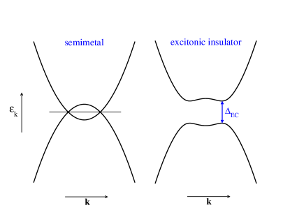
Figure 1: Schematic picture of excitonic condensation in a semimetal. Left: The band structure of a semimetal with overlapping bands and no inter-band hybridisation. Right: The band structure of an excitonic insulator with a gap opened by the Weiss field $\Delta_{\text{EC}}$.

Excitonic condensation denotes spontaneous coherence between valence and conduction electrons that arises as a consequence of electron-electron interaction. As such, it is usually represented by orbital or band off-diagonal elements of one-particle density matrix, which possess finite expectation values below the transition temperature $T_{c}$. It was originally proposed Mott (1961); Knox (1963) to take place in the vicinity of semimetal-semiconductor transition depicted in Fig. 1. In an idealised system where the number of particles in the valence and conduction bands is separately conserved, the excitonic condensation breaks this symmetry and fixes the relative phase of valence and conduction electrons. Since inter-band hybridisation or pair- and correlated-hopping terms in the electron-electron interaction, which mix the valence and conduction bands, inevitably exist in real materials the excitonic condensation in the above sense is always an approximation. The closest realisation of this idealised exciton condensate (EC) can be found in bi-layer systems. In typical bulk structures, where the conduction-valence charge conservation does not hold and thus the relative phase of valence and conduction electrons is not arbitrary, the excitonic condensation reduces to breaking of lattice symmetries, e.g., leading to electronic ferroelectricity Batista (2002), and/or gives rise to exotic magnetic orders characterised by higher-order multipoles. The concept of EC allows unified description and understanding of these transitions.

The theory of excitonic condensation was developed in 1960’s and 1970’s with weakly correlated semimetals and semiconductors in mind. More recently the ideas of excitonic condensation were applied to strongly-correlated systems described by Hubbard-type models. In their strong-coupling limit, these models lead to spin or hard-core boson problems that have been studied in other contexts. The purpose of this topical review is to summarise the recent work on the excitonic condensation in Hubbard-type models, discuss the corresponding phase diagram and describe connections to various other models such as the Blume-Emmery-Griffiths Blume, Emery, and Griffiths (1971), bosonic $t$-$J\,$or bi-layer Heisenberg Sachdev and Bhatt (1990) models. In particular, we aim at providing a ’dictionary’ for the names of mutually corresponding phases found in different models. We only briefly touch the active field of bi-layer systems in Sec. V.2 and the spectacular transport phenomena observed there and refer the reader to specialised literature. We completely omit another major direction of the exciton-polariton condensation Byrnes, Kim, and Yamamoto (2014).

I.1 Brief history of the weak-coupling theory of excitonic condensation

In 1961 Mott Mott (1961) considered metal-insulator transition in a divalent material (even number of electrons per unit cell) associated with continuous opening of a gap, e.g., due to application of external pressure. He argued that the one-electron picture cannot be correct, that a semimetal with small concentration of electrons and holes will be unstable if electron-hole interaction is taken into account. Knox Knox (1963) approached the transition from the insulator side and argued that if the excitonic binding energy overcomes the band gap the system becomes unstable. These proposals were put into a formal theory by Keldysh and Kopaev Keldysh and Kopaev (1965), and des Cloizeaux des Cloizeaux (1965) who developed a weak-coupling Hartree-Fock theory of excitonic condensation analogous to the BCS theory of superconductivity. The role of the pairing glue is played by the inter-band Coulomb interaction, which favours formation of bound electron-hole pairs, excitons. The early theories employed so called dominant term approximation, which consists in keeping only the density-density intra- and inter-band terms of the Coulomb interaction. This approximation appears well justified for weakly correlated metals or semiconductors where the pair glues arise from the long-range part of the interaction. It leads to a large manifold of degenerate excitonic states. It is due to this degeneracy that the small and so far neglected exchange and pair-hopping interaction terms may play an important role. Halperin and Rice Halperin and Rice (1968a) showed that these terms select one out of the four following states as the lowest one: charge-density wave charge-current-density wave, spin-density-wave and spin-current-density wave.

In 1970’s Volkov and collaborators showed in a series of articles Volkov and Kopaev (1973); Volkov, Kopaev, and Rusinov (1975); Volkov, Rusinov, and Timerov (1976) that excitonic condensation in slightly off-stoichiometric systems leads to formation of a uniform ferromagnetic state although the normal state does not exhibit a magnetic instability. The idea of an excitonic ferromagnet was revived at the beginning of 2000’s in the context of hexaborides, Sec. V.1.

II Spinless fermions

Before discussing the two band Hubbard model (7), we look at its spinless version

$$\begin{split}H_{\text{EFK}}=&\sum_{\langle ij\rangle}\left(t_{a}a_{i}^{\dagger}a^{\phantom{\dagger}}_{j}+t_{b}b_{i}^{\dagger}b^{\phantom{\dagger}}_{j}\right)+H.c.\\ +&\sum_{\langle ij\rangle}\left(V_{ab}b_{i}^{\dagger}a^{\phantom{\dagger}}_{j}+V_{ba}a_{i}^{\dagger}b^{\phantom{\dagger}}_{j}\right)+H.c.\\ +&\frac{\Delta}{2}\sum_{i}\left(n^{a}_{i}-n^{b}_{i}\right)+\tilde{U}\sum_{i}n^{a}_{i}n^{b}_{i},\end{split}$$ (1)

which describes electrons of two flavours ($a$ and $b$) moving on a lattice and interacting via an on-site interaction. Here, $a_{i}^{\dagger}$ ($a^{\phantom{\dagger}}_{i}$) is an operator creating (annihilating) a fermion of flavour $a$ on lattice site $i$, $n_{i}^{a}=a_{i}^{\dagger}a^{\phantom{\dagger}}_{i}$ is the corresponding local density operator, and analogically for $b$ fermions. We will use $\psi_{a}(\mathbf{r})$ and $\psi_{b}(\mathbf{r})$ to refer to the density distribution around the lattice sites in orbitals $a$ and $b$, respectively, when necessary. The sum $\sum_{\langle ij\rangle}$ runs over the nearest neighbour (nn) bonds. Model (1) is usually called extended Falicov-Kimball model (EFKM), where ’extended’ implies that both $t_{a},t_{b}\neq 0$. In the original Falicov-Kimball model (FKM) Falicov and Kimball (1969), $t_{b}=V_{ab}=V_{ba}=0$, only the $a$-electrons can propagate while the ’heavy’ $b$-electrons are immobile. 

Three versions of EFKM have been discussed in the literature in the context of excitonic condensation: (i) FKM with $t_{b}=V_{ab}=V_{ba}=0$, (ii) EFKM without cross-hopping $V_{ab}=V_{ba}=0$ and (iii) EFKM with cross-hopping $V_{ab},V_{ba}\neq 0$. Since the conservation of the charge per flavour plays a central role in excitonic condensation we compare models (i)-(iii) from that perspective. Hamiltonian (1) conserves the total charge for any choice of parameters. Since the corresponding $U(1)$ symmetry is not broken in any phase considered here, we will not mention this symmetry explicitly in the text. The FKM (i) conserves the number of the heavy $b$-electron on each site, which gives rise to a local $U(1)$ gauge symmetry. Finite $t_{b}$ in (ii) removes the local gauge invariance, but preserves independently the number of $a$- and $b$-electrons, which gives rise to a global $U(1)$ symmetry associated with the arbitrariness of the relative phase of the $a$- and $b$-electrons. Finally, finite cross-hopping in (iii) removes this $U(1)$ symmetry. An important special case of (iii) is a system with a site symmetry that prohibits an on-site $a-b$ hybridisation. As an example, we may consider orbitals $a$ and $b$ of different parity, which implies $V_{ab}=-V_{ba}$. In this case, the $U(1)$ symmetry is not removed completely but reduced to a discrete $Z_{2}$ symmetry reflecting the invariance of (1) under the transformation $a_{i}\rightarrow-a_{i}$, $V_{ab}\leftrightarrow V_{ba}$.

On a bipartite lattice there are additional symmetries. Models (ii) with $t_{a}t_{b}>0$ and $t_{a}t_{b}<0$ can be mapped on each other by $a_{i}\rightarrow(-1)^{i}a_{i}$ . In the EC phase the map turns ferro-EC order ($t_{a}t_{b}<0$) into an antiferro-EC order ($t_{a}t_{b}>0$). This property will be important for understanding the nature of EC phase in FKM ($t_{a}t_{b}=0$), which lies between the ferro- and antiferro- phases. There is also a symmetry with respect to the sign of $\Delta$ for $|t_{a}|=|t_{b}|$ consisting in the exchange $a_{i}\leftrightarrow b_{i}$.

Model (ii) with symmetric bands $t_{a}=t_{b}$ is identical to a single band Hubbard model, where flavours $a$ and $b$ play the role of the spin variable and $\Delta$ stands for an external magnetic field.

Model (ii) with $t_{a}=-t_{b}$ is identical to the single band Hubbard model with attractive interaction. The corresponding mapping is achieved by particle-hole transformation in one of the bands $b^{\phantom{\dagger}}_{i}\leftrightarrow b^{\dagger}_{i}$ and reversing the sign of the interaction $\tilde{U}\rightarrow-\tilde{U}$. This transformation maps an excitonic insulator onto an $s$-wave superconductor. Note that crystal-field $\Delta$ in the excitonic insulator plays the role of chemical potential in the superconductor and the chemical potential in the excitonic insulator plays the role of magnetic field in the superconductor. This shows that deviations from half-filling are detrimental for EC in the same way magnetic field is for spin-singlet superconductivity. The mapping between the superconductor and excitonic insulator obviously breaks down in the presence of external electro-magnetic field.

II.1 Falicov-Kimball model

The interest in excitonic condensation in FKM started with the work of Portengen et al. Portengen, Östreich, and Sham (1996a, b) who studied FKM model augmented with the hybridisation between the heavy $b$-electrons and light $a$-electrons $V_{ab}=-V_{ba}\neq 0$. Using self-consistent mean-field (BCS-like) theory they found solutions with spontaneous on-site hybridisation – excitonic condensate. They showed that in case that the $a$ and $b$ orbitals are of opposite parity the excitonic condensation gives rise to a ferroelectric polarisation. Importantly, their excitonic condensate existed also in the limiting case of $V_{ab}=V_{ba}=0$ suggesting a new ground state of the original FKM. This result was challenged by subsequent theoretical studies Czycholl (1999); Farkašovský (1999, 2002); Brydon et al. (2005) of FKM in one and infinite dimension, which found no spontaneous hybridisation. It was pointed out that the method of Portengen and collaborators missed competing ordered states and the possibility of phase separation. Freericks and Zlatić Freericks and Zlatić (2003) argued that spontaneous hybridisation in FKM breaks the local $U(1)$ gauge symmetry, associated with the phase of the heavy electron, and thus is prohibited by Elitzur’s theorem Elitzur (1975). The question is, however, quite subtle as can be illustrated, for example, by the excitonic susceptibility in $d=\infty$ FKM, which has a logarithmic singularity at $T=0$ Zlaticć et al. (2001). The insight into the issue can be provided by going into EFKM. The mapping between $t_{b}t_{a}>0$ and $t_{a}t_{b}<0$ models (on bipartite lattice) implies that if there is an (ferro-) ordered state in the limit $t_{b}\rightarrow 0^{-}$ there must an antiferro- order in the limit $t_{b}\rightarrow 0^{+}$ and thus FKM is an unstable point between these two phases.

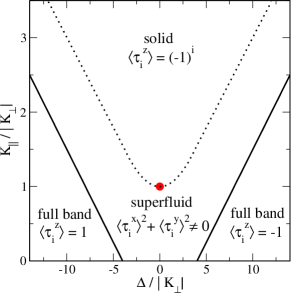
Figure 2: The $T=0$ phase diagram of the $d=2$ $XXZ$ model constructed from data of Ref. Schmid et al., 2002. The dotted line marks the first-order solid-superfluid boundary, the full lines denote the continuous transitions between the superfluid and the fully polarised state.

II.2 Extended Falicov-Kimball model

II.2.1 Strong-coupling limit

An alternative way to EC order in FKM is to make both fermion species mobile, i.e., introducing EFKM. Batista Batista (2002) studied EFKM at half-filling in the strong coupling limit $\tilde{U}\gg t_{a},t_{b}$ as an alternative way to electronic ferroelectricity. Introducing pseudo spin variables

$$\tau_{i}^{x} =a_{i}^{\dagger}b_{i}^{\phantom{\dagger}}+b_{i}^{\dagger}a_{i}^{\phantom{\dagger}},\quad\tau_{i}^{y}=i(b_{i}^{\dagger}a_{i}^{\phantom{\dagger}}-a_{i}^{\dagger}b_{i}^{\phantom{\dagger}}),$$ (2)

$$\tau_{i}^{z} =a_{i}^{\dagger}a_{i}^{\phantom{\dagger}}-b_{i}^{\dagger}b_{i}^{\phantom{\dagger}},$$

he arrived at a strong-coupling effective Hamiltonian, which in the case $V_{ab}=V_{ba}=0$ reads

$$\mathcal{H}_{\text{eff}}=\frac{1}{2}\sum_{\langle ij\rangle}\left(K_{\parallel}\tau_{i}^{z}\tau_{j}^{z}+K_{\perp}\left(\tau_{i}^{x}\tau_{j}^{x}+\tau_{i}^{y}\tau_{j}^{y}\right)\right)+\frac{\Delta}{2}\sum_{i}\tau_{i}^{z}.$$ (3)

$\mathcal{H}_{\text{eff}}$ acts in the low-energy space built of states with singly occupied sites only. The coupling constants to the lowest order in $t/\tilde{U}$ read $K_{\parallel}=\tfrac{t_{a}^{2}+t_{b}^{2}}{\tilde{U}}$ and $K_{\perp}=\tfrac{2t_{a}t_{b}}{\tilde{U}}$. Labelling the two local states $|\uparrow_{i}\rangle=a_{i}^{\dagger}|0\rangle$ and $|\downarrow_{i}\rangle=b_{i}^{\dagger}|0\rangle$ the structure of the $S=1/2$ $XXZ$-model in an external field along the $z$-axis is apparent. Note that while $K_{\perp}$ can be both positive and negative, $K_{\parallel}$ is always positive. There is a well-known exact mapping of (3) onto the model of spinless hard-core bosons Matsubara and Matsuda (1956)

$$\tilde{\mathcal{H}}_{\text{eff}}=\epsilon\sum_{i}n_{i}+K_{\perp}\sum_{\langle ij\rangle}\left(d^{\dagger}_{i}d^{\phantom{\dagger}}_{j}+H.c.\right)+2K_{\parallel}\sum_{\langle ij\rangle}n_{i}n_{j},$$ (4)

with $\epsilon=\Delta-zK_{\parallel}$ ($z$ is the number of nearest neighbours). The operator $d^{\dagger}_{i}$ ($d^{\phantom{\dagger}}_{i}$) creates (annihilates) a boson on site $i$, and $n_{i}=d^{\dagger}_{i}d^{\phantom{\dagger}}_{i}$ is the local density operator. The physical states are constrained to those containing zero or one bosons per site. In this language, the $|\downarrow_{i}\rangle$ is the local bosonic vacuum and $|\uparrow_{i}\rangle=d^{\dagger}_{i}|\downarrow_{i}\rangle$ is a state with one boson. The transverse spin coupling translates into bosonic hopping, the longitudinal coupling into nearest-neighbour repulsion and the magnetic field into bosonic chemical potential. Moving between the spin and boson formulation has been traditionally used to allow convenient treatment of various models Holstein and Primakoff (1940); Auerbach (1993).

The model (3,4) is much studied in the context of cold atoms on optical lattices. Its $T=0$ phase diagram for a square lattice is shown in Fig. 2. Besides the trivial phases obtained for large $|\Delta|$, which correspond to orbitals of one flavour being filled and the other empty (saturated spin polarisation along the $z$-axis), there are two more phases. The solid phase ($z$-axis Néel antiferromagnet) favoured by $K_{\parallel}$, and the superfluid phase ($xy$ magnetic order) favoured by $K_{\perp}$. The solid phase is characterised by checker-board arrangement of sites with occupied $a$ and $b$ orbitals. The solid phase is connected to the ground state of half-filled FKM Brandt and Mielsch (1989). The superfluid phase is characterised by a finite expectation value $\langle d_{i}\rangle$, i.e., can be described as a condensate of the $d$-bosons. In the language of the EFKM this means a finite $\langle a_{i}^{\dagger}b_{i}\rangle$ expectation value characterising the excitonic condensate. To understand the phase diagram in Fig. 2 one may start form the familiar point of Heisenberg antiferromagnet, $\Delta=0$, $K_{\perp}=K_{\parallel}$. Upon application of a magnetic field ($-\Delta$) the ordered moments pick an arbitrary perpendicular orientation with a small tilt in the field direction (superfluid). For $|K_{\perp}|>K_{\parallel}$ the in-plane order is obtained without the external field, while for $|K_{\perp}|<K_{\parallel}$ a finite field is needed to destroy the Ising (solid) order.

The solid and superfluid phases have quite different properties. The solid phase breaks the discrete translational symmetry. The superfluid phase breaks continuous $U(1)$ symmetry associated with the phase of $d$-boson. For $K_{\perp}>0$ the superfluid also breaks the translational symmetry with the phase of $\langle d_{i}\rangle$ varying between sublattices. Therefore in two dimensions only solid long-range order exists at finite temperature Mermin and Wagner (1966), while the superfluid phase has the form of Kosterlitz-Thouless phase Berezinskii (1972); Kosterlitz and Thouless (1973). The mismatch between the symmetries of solid and superfluid phases implies a first-oder transition between them or existence of an intermediate supersolid phase where both the orders are present. The stability of the supersolid phase is a much studied question in the context of model (4) and its generalisations. Investigations on cubic lattice in two Schmid et al. (2002) and three Fisher and Nelson (1974) dimensions found the first-order transition scenario to be realised. However, a robust supersolid phase was found on the triangular lattice Melko et al. (2005); Heidarian and Damle (2005); Boninsegni and Prokof’ev (2005); Wessel and Troyer (2005). Existence of a supersolid on triangular lattice is related to the fact that the solid and the superfluid adapt differently to the geometrical frustration. For further reading on hard-core boson we refer the reader to specialised literature.

We conclude this section by considering the effect of cross-hopping. Non-zero cross-hopping $V_{ab},V_{ba}$ in (1) breaks the $U(1)$ symmetry of EFKM and generates additional terms in Hamiltonian (4) Batista (2002). These are of two types. First, the ’correlated-hopping’ terms of the form $(d_{i}^{\phantom{\dagger}}+d_{i}^{\dagger})(2n_{j}^{\phantom{\dagger}}-1)$ and of the order $(V_{ab}t_{a}-V_{ba}t_{b})/\tilde{U}$. Summed over the nn sites their contribution can be split into a source field for $d$-bosons, proportional to the mean boson density $\langle n\rangle$, and a coupling of $d_{i}^{\phantom{\dagger}}+d_{i}^{\dagger}$ to the density fluctuations. With a finite source field the situation is analogous to a ferromagnetic transition in an external magnetic field, i.e., the sharp transition is smeared out and diminishes completely if the external field is comparable or larger than the internal (Weiss) fields. In some symmetries the contributions of individual neighbours to the source fields add up to zero, e.g., in the case of $a$- and $b$-orbitals in (1) of different parity Batista (2002). In this case, phase transition is still possible. However, the second type of terms generated by cross-hopping of the form $d_{i}^{\phantom{\dagger}}d_{j}^{\phantom{\dagger}}$ and $d_{i}^{\dagger}d_{j}^{\dagger}$ and of the order $V_{ab}V_{ba}/\tilde{U}$ reduce the symmetry of the system to $Z_{2}$. Depending on the sign of this term the order parameter $\langle d_{i}^{\dagger}\rangle=\langle a_{i}^{\dagger}b_{i}\rangle$ is either real or imaginary. The meaning of the phase of the order parameter $\langle a_{i}^{\dagger}b_{i}\rangle$ was discussed by Halperin and Rice Halperin and Rice (1968a). In case or real orbitals $\psi_{a}(\mathbf{r})$ and $\psi_{b}(\mathbf{r})$, real $\langle a_{i}^{\dagger}b_{i}\rangle$ gives rise to charge density modulation while imaginary $\langle a_{i}^{\dagger}b_{i}\rangle$ gives rise to periodic current pattern. In a model with inversion symmetry about the lattice sites, studied in Ref. Batista, 2002, $V_{ab}=-V_{ba}$ leads to real $\langle a_{i}^{\dagger}b_{i}\rangle$ implying an Ising-like ferroelectric transition. Solution with purely imaginary $\langle a_{i}^{\dagger}b_{i}\rangle$ was reported in $d=1$ EFKM by Sarasua and Continentino Sarasua and Continentino (2004) for somewhat artificial choice of purely imaginary $V_{ab}=V_{ba}$.

II.2.2 Intermediate and weak coupling

Studies using various techniques and in different dimenssionalities, reviewed below, lead to the conclusion that the behaviour observed in the strong-coupling limit of EFKM extends to the intermediate coupling and connects to the weak-coupling regime. To be able to compare these results we have to understand how they are interpreted, in particular in $d=1,2$. Following the Mermin-Wagner theorem Mermin and Wagner (1966), the superfluid, which breaks continuous symmetry, is characterised by long-range order at finite $T$ in $d=3$, by long-range order at $T=0$ and algebraic correlations at finite $T$ in $d=2$, and by algebraic correlations at $T=0$ in $d=1$. In the Ising-like solid phase a long-range order exists at finite $T$ in $d=2,3$, while in $d=1$ there is a long-range order at $T=0$. The onset of algebraic correlations was used as a criterion to define the transition to the superfluid phase in the $d=1,T=0$ Monte-Carlo studies Batista et al. (2004). Mean-field techniques on the other hand do not distinguish dimenssionalities and long-range order is obtained even if it does not exist in the exact solution. In these cases one compares the onset of algebraic correlations in more rigorous methods with the onset of mean-field long-range order.

Using the constrained path Monte-Carlo method Batista et al. Batista et al. (2004) obtained the $T=0$ phase diagram of the $d=1,2$ model shown in Fig. 3. In fact, Farkašovský Farkašovský (2008) showed that self-consistent Hartree-Fock method reproduces the Monte-Carlo phase diagram in $d=2$ remarkably well (see Fig. 3) and extended the study to $d=3$ and $t_{b}\ll 1$ . A similar HF phase diagram was obtained by Schneider and Czycholl Schneider and Czycholl (2008) for semielliptic densities of states ($d=\infty$ Bethe lattice). In both studies, the excitonic phase persists in the limit $|t_{b}|\rightarrow 0$ for certain range of $\Delta$. Due to the symmetry of EFKM under $t_{b}\leftrightarrow-t_{b}$, $t_{b}=0$ is an unstable fixed point between the ferro and antiferro excitonic phases. Interestingly, for $t_{b}\sim 0$ Farkašovský Farkašovský (2008) finds also a phase where both the solid and excitonic orders are present simultaneously - a supersolid phase. This result has not been confirmed by other studies yet and the supersolid phase was shown to be unstable in the strong-coupling limit Schmid et al. (2002). Moreover, existence of a phase with finite $\langle a^{\dagger}b\rangle$ at $t_{b}=0$, which smoothly connects to both $t_{b}>0$ and $t_{b}<0$ violates the Elitzur’s theorem Elitzur (1975).

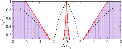
Figure 3: The $T=0$ phase diagram of $d=2$ EFKM for $\tilde{U}/t_{a}=2$ obtained with constrained path Monte-Carlo Batista et al. (2004) (top) and Hartree-Fock approximation Farkašovský (2008) (bottom). The $\alpha$ and $\varepsilon$ (violet shaded) phases correspond to filled $b$ and $a$ band, respectively. The solid $\gamma$ phase (grey shaded) is surrounded by the excitonic (superfluid) phase $\beta$. The supersolid $\beta^{\prime}$ was not found in the Monte-Carlo simulations on square lattice. The dotted lines in the top panel represent the strong-coupling phase boundaries of Fig. 2. The bottom panel was adapted with permission of author from Ref. Farkašovský, 2008. Copyrighted by the American Physical Society.

II.2.3 BCS-BEC crossover

The similarity of the strong- and weak-coupling phase diagrams opens an interesting question of how the physics described by the the hard-core bosons (3) evolves into the Hartree-Fock physics of fermions in (1). Similar question is known as the BCS-BEC crossover in the context of superconductivity or crossover between Slater and Heisenberg antiferromagnet. The issue of BCS-BEC crossover in the excitonic phase of half-filled EFKM was studied by several authors using random phase approximation (RPA) Zenker et al. (2012), slave-boson Zenker et al. (2010, 2011), projective renormalisation Phan, Becker, and Fehske (2010), variational cluster Seki, Eder, and Ohta (2011), exact diagonalisation Kaneko et al. (2013a), and density-matrix renormalisation group Ejima et al. (2014) techniques. The different methods provide quite consistent picture of the phase diagram with the provision that long-wavelength fluctuations of the order parameters are ignored by some of the mean-field methods, which therefore describe critical phase in $d=1,T=0$ and the Kosterlitz-Thouless phase in $d=2$ as phases with true long-range order.

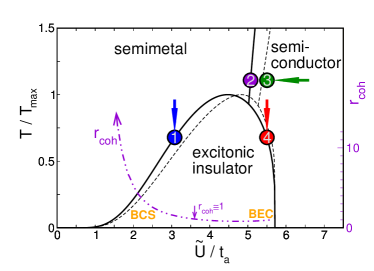
Figure 4: The phase diagram of $d=2$ half-filled EFKM for $\Delta=2.4$, $t_{a}=1$, $t_{b}=-0.8$ obtained with RPA (solid lines) and slave bosons (dashed lines). Note that the temperature is scaled to the maximum critical temperature $T_{\text{max}}$, where $T_{\text{max}}=0.361$ (RPA) and $T_{\text{max}}=0.256$ (slave bosons). The points marked 1-4 are discussed in the text. Adapted with permission of authors from Ref. Zenker et al., 2012. Copyrighted by the American Physical Society.

The BCS vs BEC question can be formulated as: Are there long-lived excitons above $T_{c}$ that condense at the transition? The typical $T-U$ phase diagram of half-filled EFKM with exciton condensate is shown in Fig. 4. Following Ref. Zenker et al., 2012 we introduce a boson creation operator $d_{\mathbf{q}}^{\dagger}=\tfrac{1}{\sqrt{N}}\sum_{\mathbf{k}}a_{\mathbf{k}+\mathbf{q}}^{\dagger}b^{\phantom{\dagger}}_{\mathbf{k}}$ and the corresponding propagator $\chi^{ab}_{\mathbf{q}}(\omega)=\langle\langle d^{\phantom{\dagger}}_{\mathbf{q}};d^{\dagger}_{\mathbf{q}}\rangle\rangle_{\omega}$. The excitonic transition proceeds differently on the semi-metal and semi-conductor sides. In semimetal, the particle-hole continuum extends to zero energy in a finite $\mathbf{q}$-region of the Brillouin zone. While long-lived excitons may exist in some other parts of the Brillouin zone (Fig. 5b), they are not the lowest energy excitations and the excitonic transition follows the BCS scenario. In semiconductor, the excitonic band in the two-particle spectrum extends throughout the whole Brillouin zone (Fig. 5e-g) and lies below the particle-hole continuum. $B_{\mathbf{q}}(\omega)$ , the coherent part of $\operatorname{Im}\chi^{ab}_{\mathbf{q}}(\omega)$, can be approximated as

$$B_{\mathbf{q}}(\omega)=-\pi Z_{X}(\mathbf{q})\delta(\omega-\omega_{X}(\mathbf{q})),$$ (5)

where $Z_{X}(\mathbf{q})$ is the weight of the excitonic quasiparticle and $\omega_{X}(\mathbf{q})$ is its dispersion. Note that both $Z_{X}(\mathbf{q})$ and $\omega_{X}(\mathbf{q})$ depend on temperature. The number of excitons with crystal-momentum $\mathbf{q}$ is given by

$$N_{X}(\mathbf{q})=Z_{X}(\mathbf{q})n_{\text{BE}}(\omega_{X}(\mathbf{q})),$$ (6)

where $n_{\text{BE}}(\omega)$ is the Bose-Einstein (BE) function. The excitonic transition in a semiconductor is connected with the minimum of $\omega_{X}(\mathbf{q})$ going to zero at $T_{c}$ and the resulting divergence of $N_{X}(\mathbf{q})$, Fig. 6.

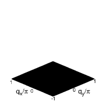
(a) $\tilde{U}=0.50$,
$T/T_{\text{max}}=1.108$

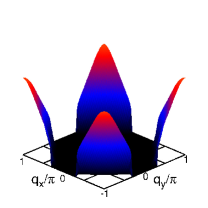
(b) $\tilde{U}=3.08$,
$T/T_{\text{max}}=0.679$

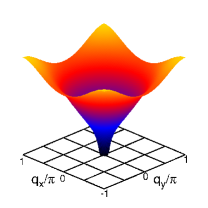
(c) $\tilde{U}=5.07$,
$T/T_{\text{max}}=1.108$

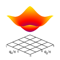
(d) $\tilde{U}=5.50$,
$T/T_{\text{max}}=1.108$

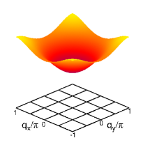
(e) $\tilde{U}=5.50$,
$T/T_{\text{max}}=0.679$

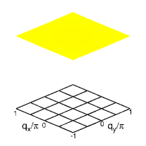
(f) $\tilde{U}=50.0$,
$T/T_{\text{max}}=1.108$

Figure 5: Evolution of the exciton quasiparticle weight $Z_{X}(\mathbf{q})$, obtained with RPA, across the semimetal–semiconductor crossover. On the metallic side (a-c) non-zero $Z_{X}(\mathbf{q})$ exists only in a part of the Brillouin zone. On the semiconductor side (e-g), $Z_{X}(\mathbf{q})$ is finite everywhere in the Brillouin zone and approaches $Z_{X}(\mathbf{q})=1$ in the strong-coupling limit (g). Panel (a) corresponds to a weakly coupled semimetal with no excitonic quasi-particle residues anywhere in the Brillouin zone. Panels (b)-(f) correspond to the points 1-4 of Fig. 4. Adapted with permission of authors from Ref. Zenker et al., 2012. Copyrighted by the American Physical Society.

The semimetal and semiconductor side of the phase diagram appear to be qualitatively different. It is therefore instructive to see that the evolution from a semimetal to a semiconductor with increasing $\tilde{U}$ is in fact smooth although they differ by the presence of the excitonic band. The key observation is that the parts of the exciton band that split off the particle-hole continuum carry little spectral weight $Z_{X}(\mathbf{q})$. Moreover, the notion of infinitely sharp $B_{\mathbf{q}}(\omega)$ is an idealisation, which holds only for excitonic peak well separated from the particle-hole continuum. Fig. 5 shows the evolution of $Z_{X}(\mathbf{q})$. Starting from a semimetal with no exciton band, through a semimetal with exciton band in a part of the Brillouin zone, the region of $Z_{X}(\mathbf{q})=0$ shrinks to a point at the semimetal/semiconductor crossover. On the semiconductor side, $Z_{X}(\mathbf{q})$ remains finite over the entire Brillouin zone. Vanishing of the excitonic insulator for large $\tilde{U}$ is the consequence of $\omega_{X}(\mathbf{q})>0$ being finite for all $\mathbf{q}$ down to $T=0$.

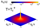
Figure 6: The occupancy of the excitonic states $N_{X}(\mathbf{q})$ at points 3 (left panel) and 4 (right panel) of Fig. 4 on the semiconductor side of the phase diagram. The diverging occupancy of the lowest mode, $\mathbf{q}=(0,0)$, at $T_{c}$ is clearly visible. Adapted with permission of authors from Ref. Zenker et al., 2012. Copyrighted by the American Physical Society.

Another question worth understanding is the relationship of the present picture to the strong-coupling limit $t_{a,b}\ll\tilde{U}$. We point out that to reach this limit one cannot keep $\Delta$ fixed but have to scale it as $1/\tilde{U}$ (see also Fig. 2). Although the bosonic excitons exist in a semiconductor away from the strong-coupling limit, there is no separation of the bosonic and fermionic energy scales. This is reflected in the $Z_{X}(\mathbf{q})$ substantially different from 1. The dynamics of the excitons therefore cannot be described by purely bosonic Hamiltonian. One has the option to keep the fermions in the model, use a more general action description of the exciton dynamics or resort to an effective bosonic Hamiltonian describing only the vicinity of the minimum of the exciton band. While the particle-hole gap grows linearly with increasing $\tilde{U}$, the exciton band remains located around $\Delta$ with its width approaching the $t_{a}t_{b}/\tilde{U}$ scaling. If the particle-hole gap is sufficiently large, the excitons are no more dressed with the particle-hole excitations and thus $Z_{X}(\mathbf{q})\approx 1$ everywhere in the Brillouin zone. The exciton dynamics in this limit is described by purely bosonic Hamiltonian (4).

III Two-band Hubbard model (S=1/2 fermions)

The two-band Hubbard model (2BHM) generalises EFKM (1) to include electron spin. In absence of external magnetic field and spin-orbit coupling the one-particle part $H_{\text{t}}$ consists of two identical copies of the corresponding terms in EFKM. The interaction part $H_{\text{int}}$ is richer.

$$H_{\text{2BH}}= H_{\text{t}}+H_{\text{int}}$$ (7)

$$H_{\text{t}}= \sum_{\langle ij\rangle,\sigma}\left(t_{a}a_{i\sigma}^{\dagger}a^{\phantom{\dagger}}_{j\sigma}+t_{b}b_{i\sigma}^{\dagger}b^{\phantom{\dagger}}_{j\sigma}\right)+H.c.$$

$$+ \sum_{\langle ij\rangle,\sigma}\left(V_{ab}b_{i\sigma}^{\dagger}a^{\phantom{\dagger}}_{j\sigma}+V_{ba}a_{i\sigma}^{\dagger}b^{\phantom{\dagger}}_{\j\sigma}\right)+H.c.$$

$$+ \frac{\Delta}{2}\sum_{i,\sigma}\left(n^{a}_{i\sigma}-n^{b}_{i\sigma}\right)$$

$$H_{\text{int}}= U\sum_{i}\left(n^{a}_{i\uparrow}n^{a}_{i\downarrow}+n^{b}_{i\uparrow}n^{b}_{i\downarrow}\right)+U^{\prime}\sum_{i,\sigma\sigma^{\prime}}n^{a}_{i\sigma}n^{b}_{i\sigma^{\prime}}$$

$$- J\sum_{i\sigma}\left(n^{a}_{i\sigma}n^{b}_{i\sigma}+a_{i\sigma}^{\dagger}a_{i\bar{\sigma}}^{\phantom{\dagger}}b_{i\bar{\sigma}}^{\dagger}b_{i\sigma}^{\phantom{\dagger}}\right)$$

$$+ J^{\prime}\sum_{i}\left(a_{i\uparrow}^{\dagger}a_{i\downarrow}^{\dagger}b_{i\downarrow}^{\phantom{\dagger}}b_{i\uparrow}^{\phantom{\dagger}}\right)+H.c.,$$

with the notation $\bar{\sigma}=-\sigma$. There are two general set-ups in which EC in 2BHM have been studied: a lattice of two-orbital atoms and a bi-layer Hubbard model system.

In the bi-layer model the orbitals $a_{i}$ and $b_{i}$ are assumed to be spatially well separated and the exchange-interaction is vanishingly small $J^{\prime},J\approx 0$. This is equivalent to the dominant-term approximation used extensively for long-range interaction Halperin and Rice (1968a). Similarly the on-site and inter-site inter-layer tunnelling, $V_{ab},V_{ba}\approx 0$, is negligible due to the spatial separation of layers.

In two-orbital atoms, the overlap of (orthogonal) $a$ and $b$ orbitals gives rise to a sizeable ferromagnetic Hund’s exchange $J$ and pair hopping $J^{\prime}$. The on-site $a$-$b$ hopping vanishes either by symmetry or can be eliminated by a basis transformation. The cross-hopping $V_{ab}$, $V_{ba}$ is in general non-zero, however, in materials with high symmetry it may vanish as well. .

III.1 Normal state

Before discussing the ordered phases we briefly summarise the basic properties of half-filled 2BHM without broken symmetry. Its physics at strong and intermediate coupling is controlled by competition between the Hund’s coupling $J$ and the crystal-field splitting $\Delta$ Werner and Millis (2007); Suzuki, Watanabe, and Ishihara (2009). Large $\Delta$ favours the singlet low-spin (LS) state, while large $J$ favours the triplet high-spin (HS) state, see Fig. 7. For finite $J$ the phase diagram, shown in Fig. 7, contains three regions: HS Mott insulator connected to the limit $U\gg W$, with $W$ standing for the bare bandwidth, and $J\gg\Delta$, LS band insulator connected to the limit $\Delta\gg W,U$ and a metal connected to the non-interacting limit and $\Delta<W$. The low-energy physics deep in the Mott phase is described by $S=1$ Heisenberg model with anti-ferromagnetic interaction. The band insulator far away from the phase boundaries is a global singlet separated by large gap from the excited states. In the vicinity of the HS-LS crossover both LS and HS states have to be taken into account. The physics arising in this parameter region is the subject of subsequent sections.

The physics of the $J,J^{\prime}=0$ model is different. This setting corresponds to a bi-layer system where one would typically choose $U>U^{\prime}$. In this case, the low-energy physics for $W\ll U$ and $\Delta\ll(U-U^{\prime})$ is described by $S=1/2$ bi-layer Heisenberg model, while for $\Delta\gg(U-U^{\prime})$ one obtains a band insulator. The region $\Delta\approx(U-U^{\prime})$ is described by exciton-$t$-$J\,$model, discussed later. The choice $U=U^{\prime}$, shown in Fig. 7, is anomalous in the sense that the bi-layer Heisenberg region is absent and the region $\Delta\approx 0$ corresponds to exciton-$t$-$J\,$model with two exciton flavours.

The low-energy physics of the metallic phase is sensitive to Fermi surface nesting, in particular for weak coupling. Nesting plays an important role in some popular models, e.g., the Fermi surfaces derived from $a$ and $b$ bands are perfectly nested on cubic lattice both in $d=2$ and $d=3$.

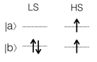
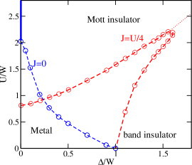
Figure 7: Left: The cartoon representation of the atomic low-spin (LS) and high-spin (HS) states. Right: The phase diagram of $d=\infty$ 2BHM with symmetric $t_{a}=t_{b}$ bands (semi-elliptic density of states) for $J^{\prime}=J=U/4$; $U^{\prime}=U-2J$ (red) and $J^{\prime}=J=0$; $U^{\prime}=U$ (blue) obtained by Werner and Millis Werner and Millis (2007). The dotted red line marks the HS-LS crossover. The vertical blue line for $J=0$ corresponds to a model with 6-fold degenerate atomic ground state. $U$ and $\Delta$ are expressed in the units of bandwidth $W$.

III.2 Excitonic order parameter

Excitonic condensation is characterised by a spontaneous coherence between the $a$- and $b$-electrons in (7), i.e., appearance of matrix elements of the form

$$F^{\sigma\sigma^{\prime}}_{ii^{\prime}}=\langle a^{\dagger}_{i\sigma}b^{\phantom{\dagger}}_{i^{\prime}\sigma^{\prime}}\rangle\quad\text{and}\quad\mathcal{F}^{\sigma\sigma^{\prime}}_{\mathbf{k}\mathbf{k}^{\prime}}=\langle a^{\dagger}_{\mathbf{k}\sigma}b^{\phantom{\dagger}}_{\mathbf{k}^{\prime}\sigma^{\prime}}\rangle.$$ (8)

These can be in general complicated objects characterised by translational symmetry, internal structure and spin symmetry.

We will consider only ordered phases with single-$\mathbf{q}$ translational symmetry, ${\mathcal{F}_{\mathbf{k}\mathbf{k}^{\prime}}\sim\delta_{\mathbf{k}^{\prime},\mathbf{k}+\mathbf{q}}}$. On the square lattice we will encounter only ferro-EC, $\mathbf{q}=0$, and antiferro-EC, $\mathbf{q}=(\pi,\pi)$ states, which correspond to uniform ${F_{ii}}$ and staggered ${F_{ii}\sim(-1)^{i}}$, respectively.

The internal structure describes the behaviour of the above matrix elements as a function of the reciprocal vector $\mathbf{k}$ or the relative position $\mathbf{R}_{i}-\mathbf{R}_{i^{\prime}}$. The internal structure reflects the symmetry of the pairing interaction. Isotropic pairing leads to isotropic $\mathcal{F}_{\mathbf{k},\mathbf{k}+\mathbf{q}}$ and, in particular, to a finite local element $F_{ii}$. Since this is the case for local Hubbard interaction (7) we can use the local element $F_{ii}$ as an order parameter for the exciton condensation. The spatial decay of the $a-b$ coherence can be quantified by a correlation length $r_{\text{coh}}$ defined as

$$r_{\text{coh}}=\sqrt{\frac{\sum_{\mathbf{R}}|\mathbf{R}|^{2}|F_{\mathbf{R}_{i},\mathbf{R}_{i}+\mathbf{R}}|^{2}}{\sum_{\mathbf{R}}|F_{\mathbf{R}_{i},\mathbf{R}_{i}+\mathbf{R}}|^{2}}}=\sqrt{\frac{\sum_{\mathbf{k}}|\nabla_{\mathbf{k}}\mathcal{F}_{\mathbf{k}\mathbf{k}}|^{2}}{\sum_{\mathbf{k}}|\mathcal{F}_{\mathbf{k}\mathbf{k}}|^{2}}}$$ (9)

was studied by several authors for EFKM Seki, Eder, and Ohta (2011); Kaneko et al. (2013a); Ejima et al. (2014) as well as 2BHM Kaneko and Ohta (2014). Since the largest contribution to the pairing interaction in these models is on-site the correlation length reflects the relative size of the pairing field to the bandwidth. Weak pairing yields sizeable $\mathcal{F}_{\mathbf{k}\mathbf{k}}$ only in the vicinity of the Fermi level and one ends with $r_{\text{coh}}$ over many unit cells (BCS limit). Strong pairing leads to almost constant $\mathcal{F}_{\mathbf{k}\mathbf{k}}$ and $r_{\text{coh}}$ limited to a few sites (BEC limit).

Finally, we discuss the spin structure of the EC order parameter, which we divide into the spin-singlet and spin-tripels parts

$$F^{\sigma\sigma^{\prime}}_{ii}=\frac{1}{2}\left(\phi_{i}^{s}\delta_{\sigma\sigma^{\prime}}+\bm{\phi}^{t}_{i}\cdot\bm{\tau}^{*}_{\sigma\sigma^{\prime}}\right),$$ (10)

i.e., singlet $\phi^{s}$ and triplet $\bm{\phi}^{t}$ components are defined by

$$\begin{split}\phi^{s}_{i}&=\sum_{\sigma}\langle a^{\dagger}_{i\sigma}b^{\phantom{\dagger}}_{i\sigma}\rangle\\ \bm{\phi}^{t}_{i}&=\sum_{\sigma\sigma^{\prime}}\langle a^{\dagger}_{i\sigma}b^{\phantom{\dagger}}_{i\sigma^{\prime}}\rangle\bm{\tau}_{\sigma\sigma^{\prime}},\end{split}$$ (11)

where $\bm{\tau}$ are the Pauli matrices and ^∗ denotes the complex conjugation. Tensorial character of $\{\phi^{s},\bm{\phi}^{t}\}$ and the fact that their elements are complex numbers allow numerous distinct phases as will be discussed in what follows. Some of the phases lead to a uniform spin polarisation while others have no ordered spin moments.

III.3 Strong-coupling limit

At half-filling and large $U,U^{\prime}\gg t_{a},t_{b},V_{ab},V_{ba},J,J^{\prime}$ the charge fluctuations are strongly suppressed. Similar to the strong-coupling treatment of EFKM, the low-energy physics can be described by an effective model built on states containing only doubly occupied sites. The virtual excitations to states with singly and triply occupied sites provide inter-site couplings in the low-energy model. Using Schrieffer-Wollf transformation to the second order one arrives at expressions of the type $t^{2}/U$, known from the analogous transformation from single-band Hubbard to Heisenberg model. By construction, the low-energy model does not capture one-particle or charge excitations, which take place only at energies of the order $U$. The general strong-coupling expressions for the case of symmetric bands $t_{a}=t_{b}$ were derived by Balents Balents (2000). In the following we discuss several special parameter choices of the strong-coupling model, which are studied in the literature.

III.3.1 Large $J$ - general formulation

For a sufficiently large Hund’s coupling $J$, the low-energy Hilbert space can be constructed from the atomic HS and LS states: ${|1\rangle=a_{\uparrow}^{\dagger}b^{\dagger}_{\uparrow}|\text{vac}\rangle}$, ${|0\rangle=\tfrac{1}{\sqrt{2}}(a_{\uparrow}^{\dagger}b^{\dagger}_{\downarrow}+a_{\downarrow}^{\dagger}b^{\dagger}_{\uparrow})|\text{vac}\rangle}$, ${|-1\rangle=a_{\downarrow}^{\dagger}b^{\dagger}_{\downarrow}|\text{vac}\rangle}$, and ${|\emptyset\rangle=b_{\uparrow}^{\dagger}b^{\dagger}_{\downarrow}|\text{vac}\rangle}$, where $|\text{vac}\rangle$ is the fermionic vacuum. The local Hilbert space is further reduced if we assume easy axis anisotropy and can drop the $|0\rangle$ state. In this case only the density-density part of the Hund’s interaction contributes.  In the following, we will derive the strong-coupling model for this case to demonstrate the principle. The generalisations are straightforward and can be found in the literature Balents (2000); Kuneš and Augustinský (2014a). Similar to (2), the low-energy Hamiltonian can be formulated in terms of pseudospin variables. Following Ref. Balents, 2000, we introduce on-site standard-basis operators Haley and Erdös (1972) $T_{i}^{mn}$ with matrix elements in the local basis

$$\langle m^{\prime}|T^{mn}|n^{\prime}\rangle=\delta_{mm^{\prime}}\delta_{nn^{\prime}}.$$ (12)

The effective Hamiltonian reads

$$\begin{split}\mathcal{H}^{(1)}_{\text{eff}}=&\epsilon\sum_{i,s}T_{i}^{ss}+K_{\perp}\sum_{\langle ij\rangle,s}\left(T_{i}^{s\emptyset}T_{j}^{\emptyset s}+i\leftrightarrow j\right)\\ +&\sum_{\langle ij\rangle,s,s^{\prime}}\left(K_{\parallel}+(-1)^{s+s^{\prime}}K_{0}\right)T_{i}^{ss}T_{j}^{s^{\prime}s^{\prime}}\\ +&K_{1}\sum_{\langle ij\rangle,s}\left(T_{i}^{s\emptyset}T_{j}^{\bar{s}\emptyset}+T_{i}^{\emptyset s}T_{j}^{\emptyset\bar{s}}\right),\end{split}$$ (13)

where $s=\pm 1$ and $\bar{s}=-s$. Typical hopping processes contributing to $\mathcal{H}^{(1)}_{\text{eff}}$ are shown in Fig. 8. The process (i) lowers the energy of HS-LS pair on nn bond relative to the LS-LS pair. Therefore it lowers the energy $\epsilon$ of a single HS site on otherwise LS lattice relative to the single atom value of $E_{HS}-E_{LS}$, and contributes to a nn repulsion between HS states $K_{\parallel}$. A similar process between two HS states with opposite $s$ gives rise to the exchange term $K_{0}$. The process (ii) exchanges the HS and LS states in a nn bond and introduces quantum fluctuations in the model. Neglecting the cross-hopping contributions (see Ref. Kuneš and Augustinský, 2014a for the general expressions including cross-hopping corrections) the coupling constants read: ${\epsilon=\Delta-3J-z\tfrac{t_{a}^{2}+t_{b}^{2}}{U^{\prime}}}$, ${K_{\perp}=\frac{2t_{a}t_{b}}{U^{\prime}}}$, ${K_{\parallel}=(t_{a}^{2}+t_{b}^{2})\tfrac{2U-U^{\prime}+2J}{U^{\prime}(U+J)}}$, and ${K_{0}=\tfrac{t_{a}^{2}+t_{b}^{2}}{U+J}}$, where $z$ is the number of nearest neighbours. Finally, the process (iii) converts HS-HS pairs with zero total moment into LS-LS pairs and vice versa. This process is possible only with finite cross-hopping, ${K_{1}=-2V_{ab}V_{ba}\tfrac{U^{\prime}}{(U+J-\Delta)(2U^{\prime}-U-J+\Delta)}}$.

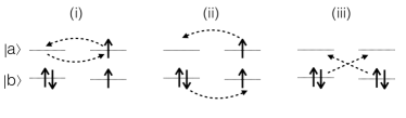
Figure 8: Typical nn hopping processes that give rise to couplings in the effective Hamiltonian (13, 15, 17).

Hamiltonian (13) can be formulated in terms of hard-core bosons. In this picture, $|\emptyset\rangle$ is identified with bosonic vacuum and $|s\rangle$ with a state containing one boson of flavour $s$. However, practical implementation of the hard-core constraint prohibiting more than one boson per site is complicated. The standard way to treat the constraint is to introduce a new vacuum state $|\Omega\rangle$ and Schwinger-like bosons: $|s\rangle=d_{s}^{\dagger}|\Omega\rangle$, $|\emptyset\rangle=h^{\dagger}|\Omega\rangle$. The physical states are required to obey the local constraint

$$h_{i}^{\dagger}h_{i}^{\phantom{\dagger}}+\sum_{s}d_{i,s}^{\dagger}d_{i,s}^{\phantom{\dagger}}=1.$$ (14)

Rewriting (13) in terms of $d$- and $h$-boson, using the replacement $T_{i}^{s\emptyset}=d_{i,s}^{\dagger}h_{i}^{\phantom{\dagger}}$ and introducing the $d$-number operator $n_{i}=\sum_{s}d_{i,s}^{\dagger}d_{i,s}^{\phantom{\dagger}}=\sum_{s}T_{i}^{ss}$ and the spin operator $S_{i}^{z}=\sum_{s}sd_{i,s}^{\dagger}d_{i,s}^{\phantom{\dagger}}=\sum_{s}sT_{i}^{ss}$ one arrives at

$$\begin{split}\tilde{\mathcal{H}}^{(1)}_{\text{eff}}&=\epsilon\sum_{i}n_{i}+K_{\perp}\sum_{\langle ij\rangle,s}\left(d^{\dagger}_{i,s}d^{\phantom{\dagger}}_{j,s}h_{j}^{\dagger}h_{i}^{\phantom{\dagger}}+H.c.\right)\\ &+K_{\parallel}\sum_{\langle ij\rangle}n_{i}n_{j}+K_{0}\sum_{\langle ij\rangle}S^{z}_{i}S^{z}_{j}\\ &-K_{1}\sum_{\langle ij\rangle,s}\left(d^{\dagger}_{i,s}d^{\dagger}_{j,\bar{s}}h_{j}^{\phantom{\dagger}}h_{i}^{\phantom{\dagger}}+H.c.\right).\end{split}$$ (15)

This allows us to interpret the $K_{\perp}$ term as nn hopping of $d$-bosons, $K_{\parallel}$ as nn repulsion between the $d$-bosons, $K_{0}$ as nn spin-spin interaction and $K_{1}$ as pairvise creation and annihilation of $d$-bosons on nn sites. Besides technical advantages, the introduction of $h$-boson for $|\emptyset\rangle$ treats the LS and HS states on equal footing and thus is well suited for $\epsilon<0$, where $|\emptyset\rangle$ is not the atomic ground state and thus cannot be viewed as the vacuum state.

The effective Hamiltonian for the case with $SU(2)$ spin symmetry has a similar structure, but differs by the presence of a third bosonic flavour $|0\rangle=d^{\dagger}_{0}|\Omega\rangle$. Introducing a cartesian vector $\mathbf{d}^{\dagger}_{i}$ with components

$$\begin{pmatrix}d^{\dagger}_{x}\\ d^{\dagger}_{y}\\ d^{\dagger}_{z}\end{pmatrix}=\frac{1}{\sqrt{2}}\begin{pmatrix}d^{\dagger}_{-1}-d^{\dagger}_{1}\\ i(d^{\dagger}_{-1}+d^{\dagger}_{1})\\ \sqrt{2}d^{\dagger}_{0}\end{pmatrix},$$ (16)

the effective Hamiltonian can be written in a compact form

$$\begin{split}\tilde{\mathcal{H}}^{(2)}_{\text{eff}}&=\epsilon\sum_{i}n_{i}+K_{\perp}\sum_{\langle ij\rangle}\left(\mathbf{d}^{\dagger}_{i}\cdot\mathbf{d}^{\phantom{\dagger}}_{j}h_{j}^{\dagger}h_{i}^{\phantom{\dagger}}+H.c.\right)\\ &+K_{\parallel}\sum_{\langle ij\rangle}n_{i}n_{j}+K_{0}\sum_{\langle ij\rangle}\mathbf{S}_{i}\cdot\mathbf{S}_{j}\\ &+K_{1}\sum_{\langle ij\rangle}\left(\mathbf{d}^{\dagger}_{i}\cdot\mathbf{d}^{\dagger}_{j}h_{j}^{\phantom{\dagger}}h_{i}^{\phantom{\dagger}}+H.c.\right)\\ &+K_{2}\sum_{\langle ij\rangle}\left(\left(\mathbf{d}_{i}^{\phantom{\dagger}}h_{i}^{\dagger}+\mathbf{d}_{i}^{\dagger}h_{i}^{\phantom{\dagger}}\right)\cdot\mathbf{S}_{j}+i\leftrightarrow j\right).\end{split}$$ (17)

Here, $\mathbf{S}_{i}$ are spin $S=1$ operators with $S^{x}_{i}=\tfrac{1}{\sqrt{2}}(T_{i}^{10}+T_{i}^{0-1}+T_{i}^{01}+T_{i}^{-10})$, $S^{y}_{i}=\tfrac{i}{\sqrt{2}}(T_{i}^{01}+T_{i}^{-10}-T_{i}^{10}-T_{i}^{0-1})$. Expressed in vector notation, $\mathbf{S}_{i}$ takes the form of a cross product

$$\mathbf{S}_{i}=-i\mathbf{d}_{i}^{\dagger}\wedge\mathbf{d}_{i}.$$ (18)

Unlike the Ising case (15) where cross-hopping is necessary to generate $K_{1}$, in the $SU(2)$ symmetric case (17) $K_{1}$ appears also without cross-hopping if the pair-hopping term is finite, $J^{\prime}\neq 0$. The last term with coupling constant $K_{2}\sim V_{ba}t_{a}+V_{ab}t_{b}$, which couples the d-operators to the spin operators, does not have an analogy in the Ising case. The full expressions for the coupling constants can be found in Ref. Kuneš and Augustinský, 2014a.

Exciton condensation in (17) is characterised by a finite expectation value $\langle\mathbf{d}^{\dagger}_{i}h_{i}\rangle$, related to the spin-triplet order parameter (11) of 2BHM by

$$\langle\mathbf{d}^{\dagger}_{i}h_{i}\rangle=\bm{\phi}^{t}_{i}/\sqrt{2}.$$ (19)

Models (15) and (17) for special choices of the coupling constants are known under their own names. We discuss these cases below.

III.3.2 Blume-Emmery-Griffiths model

Without cross-hopping and one fermionic species immobile, $t_{b},V_{ab},V_{ba}=0$, (15) becomes purely classical, with $K_{\perp},K_{1}=0$. Known as the Blume-Emmery-Griffiths (BEG) model Blume, Emery, and Griffiths (1971), it was originally introduced to describe mixtures of ³He and ⁴He. In the standard formulation of the BEG model discrete index $s$ is used to describe the local state $s=\pm 1$ corresponding to $|\pm 1\rangle$ and $s=0$ is assigned to $|\emptyset\rangle$. The model is then written as

$$H_{\text{BEG}}=\epsilon\sum_{i}s_{i}^{2}+K_{\parallel}\sum_{\langle ij\rangle}s_{i}^{2}s_{j}^{2}+K_{0}\sum_{\langle ij\rangle}s_{i}s_{j}.$$ (20)

The BEG model found its use in many areas of statistical physics. Despite its simplicity it has a rich phase diagram Hoston and Berker (1991). The phase diagram of the model on bipartite lattice does not depend on the sign of $K_{0}$ as the ferromagnetic $K_{0}<0$ and antiferromagnetic $K_{0}>0$ models can be mapped on each other by the transformation $s_{i}\rightarrow(-1)^{i}s_{i}$. For $K_{\parallel}<|K_{0}|$ there are only magnetically ordered (AFM) and normal (N) phases. At $T=0$ the N phase corresponds to empty lattice $\langle n_{i}\rangle=0$, while in the AFM phase there is one boson on each site $\langle n_{i}\rangle=1$. A typical phase diagram for $K_{\parallel}>|K_{0}|$ is shown in Fig. 9. Besides the magnetically ordered (AFM) phase there is the solid (S) phase (called antiquadrupolar in Ref. Hoston and Berker, 1991) characterised at $T=0$ by bosons occupying one sublattice, the other being empty, $\langle n_{i}\rangle=\tfrac{1}{2}(1-(-1)^{i})$. Note that this phase has a residual spin degeneracy on the occupied sites. This is a consequence of the exchange interaction beyond nn being strictly zero. In a more realistic model one expects the occupied sites to order magnetically at a sufficiently low temperature. Coexistence of the magnetic and solid order (I phase in Fig. 9 ) is found at finite temperature in a narrow range of $\epsilon$ separating the magnetic and solid phases. For positive $\epsilon$ at $T=0$, the system is in the vacuum (empty lattice). Interestingly, for moderate $\epsilon>0$ the solid phase is found at elevated temperature. This reentrant behaviour of the solid phase was found also for finite $t_{b}$ in Monte-Carlo simulations of the spinless bosons Schmid et al. (2002) as well as in DMFT simulations of 2BHM Kuneš and Křápek (2011).

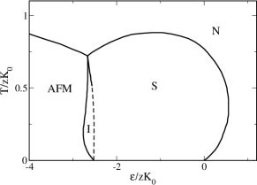
Figure 9: The phase diagram of BEG model for ${K_{\parallel}/K_{0}=3.5}$. Besides the normal phase (N), it contains the solid phase (S), antiferromagnetic phase (AFM) and ferrimagnetic phase (I). The data were taken from Ref. Hoston and Berker, 1991.

Generalisation of BEG model to the case with spin-rotational symmetry (17) is straightforward. On the mean-field level it leads to quantitative modification of the phase diagram.

III.3.3 Bosonic $t$-$J\,$model

Next, we discuss models (15) and (17) in the parameter range where they describe conserved bosons. We assume that both $a$ and $b$ electrons are mobile generating a finite hopping $K_{\perp}$ in (15) and (17) of the $d$-bosons. In addition, we require that $K_{1},K_{2}=0$, which is the case for $V_{ab},V_{ba},J^{\prime}=0$. Hamiltonians (15) and (17) describe interacting bosons carrying Ising and Heisenberg spin $S=1$, respectively. For suitable parameters, the system may undergo a BE condensation characterised by a complex vector order parameter $\bm{\phi}_{i}^{t}$ (19). In case of the Ising interaction (15) the vector $\bm{\phi}^{t}_{i}$ is confined to the $xy$ plane. The vector character of the order parameter adds additional structure to the condensation of spinless bosons discussed in Sec. II.2.1.

The role of $K_{0}$. The $SU(2)$ symmetric Hamiltonian (17) describes spinful $S=1$ bosons with infinite on-site repulsion, nn repulsion $K_{\parallel}$ and nn spin-exchange $K_{0}$. Hamiltonians of this kind have been studied both theoretically and experimentally for cold atoms in optical traps. Interestingly, in a genuine system of bosons with spin-independent interactions the structure of the exact ground state prohibits the spin-exchange from appearing in any low-energy effective Hamiltonian Eisenberg and Lieb (2002). As pointed out in Ref. Eisenberg and Lieb, 2002, it can only arise as a low-energy effective description in fermionic system - as in the present case.

BE condensation in the continuum version of (17) was studied in Refs. Ho (1998); Ohmi and Machida (1998). The sign of the exchange was shown to play a crucial role for the properties of the superfluid phase as it determines the residual symmetry of the BE condensate. Antiferromagnetic exchange ($K_{0}>0$) selects the so called polar state characterised by ${(\bm{\phi}_{i}^{t})^{*}\wedge\bm{\phi}^{t}_{i}=0}$, while ferromagnetic exchange ($K_{0}<0$) selects ferromagnetic state, where ${|(\bm{\phi}_{i}^{t})^{*}\wedge\bm{\phi}^{t}_{i}|}$ is maximised. Different residual symmetries of these states result in different low-energy dynamics and qualitatively different behaviour of topological defects (vortices) Ho (1998); Ohmi and Machida (1998). The polar and ferromagnetic phases are found for Ising spins (15) Kuneš (2014), although the topological aspects that determine the low-energy excitations and possible topological defects are different from Heisenberg spins (17).

Mean-field phase diagram. The continuum model may be viewed as an effective description of the lattice model at low boson concentrations. At higher boson concentrations other phases, e.g., these present in the BEG phase diagram Fig. 9, exist on a lattice and compete with the superfluid. In Fig. 10 we show the phase diagram of (17) on a square lattice ($z=4$) obtained with a mean-field decoupling of the pseudospin variables (13) $T_{i}T_{j}\approx\langle T_{i}\rangle T_{j}+T_{i}\langle T_{j}\rangle-\langle T_{i}\rangle\langle T_{j}\rangle$. In absence of condensed bosons, this mean-field theory reduces to that of a slightly modified BEG model (Heisenberg instead of Ising spin $S=1$) with phase boundaries marked with the red lines. The grey area marks the superfluid (exciton condensate) phase – the different shades of grey correspond to different values of $K_{\perp}$. The transition between the normal and the EC phase is continuous, while the transitions to the other ordered phases are of the first-order as dictated by symmetry. The intermediate phases, such as supersolid (with S and EC orders) or AFM-supersolid with (AFM and EC orders), which would allow continuous transitions, do not exist or are thermodynamically unstable.

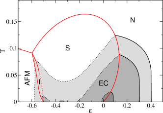
Figure 10: Mean-field $\epsilon$-$T$ phase diagram Augustinský and Kuneš of the bosonic $t$-$J\,$model (17) for the parameters: $K_{0}=0.041$, $K_{\parallel}=0.164$, and $K_{\perp}$={-0.103, -0.076, -0.023}. Solid lines mark continuous transitions, while dotted lines mark first-order transitions. The red lines correspond to the phase boundaries of the $S=1$ BEG model with its phases described in Fig. 9. The shaded regions correspond to the EC phase for the three choices of $K_{\perp}$ (with the brightest colour for largest $|K_{\perp}|$). Red lines inside the EC phase have no meaning and are shown only to put several phase diagrams in one figure.

At large $\epsilon$ the ground state is an empty lattice, a state that is connected to normal Bose gas at elevated temperatures. Upon reduction of $\epsilon$ the system undergoes a continuous transition to the superfluid EC phase with $T_{c}$ determined by $|K_{\perp}|$ and $\epsilon$. The sign of $K_{\perp}$ determines the periodicity of the order parameter: for $K_{\perp}<0$ the system goes to uniform ferro-EC state (not to be confused with ferromagnetic EC state) with $\bm{\phi}^{t}_{i}=\bm{\phi}$, while for $K_{\perp}>0$ the system goes into antiferro-EC state with $\bm{\phi}^{t}_{i}=(-1)^{i}\bm{\phi}$, the models with $\pm|K_{\perp}|$ are connected by the gauge transformation $d_{i}\rightarrow(-1)^{i}d_{i}$. The BEG phase boundaries are not affected by $K_{\perp}$.

Another parameter that determines the nature of the EC phase is the exchange coupling $K_{0}$. The phase diagram in Fig. 10 was obtained for antiferromagnetic $K_{0}>0$, but some of its features remain unchanged when the sign of $K_{0}$ is flipped. In particular, the BEG phase boundaries are unchanged. This is so because the on-site and interaction terms in the Hamiltonian are invariant under the exchange of spin species on one of the sublattices ($d_{is}\rightarrow d_{i\bar{s}}$), which maps ferromagnetic BEG to antiferromagnetic BEG model. This transformation works only for Ising spins, but in the mean-field treatment the difference between Ising and Heisenberg spins disappears. The transformation changes the hopping term in (15,17) and thus the argument cannot be used for the EC phase. Nevertheless, the mean-field phase boundary between the normal and EC phase does not depend on $K_{0}$ at all, because it contributes to the free energy in the order $\phi^{4}$. On the other hand, the first-order phase boundaries depend $K_{0}$ and its sign.

Ferromagnetic EC state. It is instructive to see where exactly the difference between the $\pm|{K_{0}}|$ models comes from. First, we point out that an order parameter of the form $\bm{\phi}^{t}_{j}=e^{i\mathbf{q}\cdot\mathbf{R}_{j}}\bm{\phi}$ implies a uniform magnetisation $\langle\mathbf{S}_{j}\rangle\sim i\bm{\phi}^{*}\wedge\bm{\phi}$ irrespective of its periodicity $\mathbf{q}$. Second, let us consider the free energy of the FMEC and polar EC states with the same magnitude $|\bm{\phi}|$ of the order parameter. The on-site, hopping and interaction terms contribute the same for the two states. However, the exchange energy in the polar EC state is zero while the FMEC state has finite exchange energy. Therefore, like in the continuum models, $K_{0}>0$ leads to a non-magnetic polar EC state, while $K_{0}<0$ leads to FMEC with a finite uniform magnetisation. For the same $|K_{0}|$, FMEC/S boundary for $K_{0}<0$ is shifted in favour of the EC phase compared to the polar-EC/S boundary for $K_{0}>0$ because the FMEC energy is lower than the corresponding polar EC energy.

Continuous transition between the FM and FMEC phases is allowed by symmetry. While we are not aware of an explicit calculation of the FM/FMEC transition for $K_{0}<0$, one can gain insight from the $T=0$ mean-field wave function, which has the product form Balents (2000)

$$|\Psi\rangle=\Pi_{i}\left(\tilde{h}h^{\dagger}+\tilde{\mathbf{d}}\cdot\mathbf{d}^{\dagger}_{i}\right)|\Omega\rangle,$$ (21)

with the coefficients fulfilling ${|\tilde{h}|^{2}+\sum_{s}|\tilde{d}^{\phantom{\dagger}}_{s}|^{2}=1}$. The magnetisation (18) in terms of the EC order parameter (19) ${\bm{\phi}=\sqrt{2}\tilde{\mathbf{d}}^{*}\tilde{h}}$ is given by

$$\langle\Psi|\mathbf{S}_{i}|\Psi\rangle=-i\tilde{\mathbf{d}}^{*}\wedge\tilde{\mathbf{d}}=\frac{i}{2|\tilde{h}|^{2}}\bm{\phi}^{*}\wedge\bm{\phi}.$$ (22)

This shows that at a continuous FMEC/FM transition $\tilde{h}$ goes to zero, while the magnetisation reaches smoothly its saturation value.

Two flavour models. We are of not aware of specific theoretical studies of spinful hard-core bosons (15,17) on a lattice. However, models (15,17) can be viewed as special cases of more general multi-component boson systems. Bosonic $t$-$J\,$model describing mixtures of two boson species with hard-core constraint have been investigated in several studies. This set-up is similar to the model (15) with Ising spin and $K_{1}=0$, which conserves both bosonic species separately. In the following, we discuss briefly how and which of the results of these studies can be used to describe (15).

The bosonic $t$-$J\,$model is usually formulated in terms of $I=1/2$ pseudospin: $I_{z}=d^{\dagger}_{1}d^{\phantom{\dagger}}_{1}-d^{\dagger}_{-1}d^{\phantom{\dagger}}_{-1}$, $I^{+}=d^{\dagger}_{1}d^{\phantom{\dagger}}_{-1}$, and $I^{-}=d^{\dagger}_{-1}d^{\phantom{\dagger}}_{1}$, and anisotropic $XXZ$ inter-site exchange interaction. While the definition of spin operator $S_{z}$ in (15) coincides with that of $I_{z}$, the transverse components $I^{+}$ and $I^{-}$ have no spin counterpart in (15). Therefore a great care is required when interpreting the results of bosonic $t$-$J\,$model in the language of model (15). In particular, the $z$-axis pseudospin order (often referred simply as an anti-ferromagnetic order) corresponds to a true spin order in (15). However, the $xy$ pseudospin order (e.g. $xy$-ferromagnet of Refs. Altman et al. (2003); Kuklov and Svistunov (2003)) does not correspond to a spin order in (15) or its $SU(2)$-symmetric generalisation (17).

Another difference between the bosonic $t$-$J\,$model and (15) concerns the hard-core constraint. In most studies on the bosonic $t$-$J\,$model simultaneous presence of two bosons of different flavour on the same site is allowed either explicitly (The hard-core constraint applies only to particles of the same species.) or implicitly (Double occupancy is allowed in the high-energy model from which the $t$-$J\,$model is derived.), giving rise to the $xy$ pseudospin exchange. On the other hand, the total hard-core constraint and the absence of the $xy$ exchange in (15) are viewed as kinematic constraints  . This calls for care when using the phase diagrams of bosonic $t$-$J\,$model since existence of some phases, e.g., the counter-superfluid of Ref. Kuklov and Svistunov (2003), depends crucially on the $xy$ exchange and so such phases are not present in (15).

In the following we discuss two types of studies on the bosonic $t$-$J\,$model, which can be translated to provide information about (15). The first concerns the transition between AFM and SF phases and the possibility of intermediate AFM-supersolid phase. Boninsegni Boninsegni (2001) and Boninsegni and Prokofév Boninsegni and Prokof’ev (2008) studied the bosonic t-J_z model, corresponding to (15) for $K_{\parallel}=-K_{0}<0$ using Monte-Carlo simulations. Since the solid phase is absent for $K_{\parallel}<|K_{0}|$ Hoston and Berker (1991), one may expect AFM-SF transition for moderate $K_{0}$ (For strong $K_{0}$ the BEG model predicts first order transition between the Mott AFM and vacuum states at low temperatures.) The Monte-Carlo calculations find a first-order AFM-SF transition with no indication of AFM-supersolid characterised by coexistence of the AFM and SF order parameters.

Numerical calculations with repulsive $K_{\parallel}$ ($K_{0}=K_{\parallel}>0$), motivated by observation of the supersolid in the spinless case, have been reported on a triangular lattice recently Trousselet, Rueda-Fonseca, and Ralko (2014); Lv, Chen, and Deng (2014). Although double occupancy by different bosonic flavours was allowed and the lattice differs from the square lattice, the basic features common to Fig. 10 were found in the phase diagram for large on-site (inter-species) repulsion. In particular, the sequence of $T=0$ phases ’empty lattice-SF-S-SF’-AFM’ with decreasing $\epsilon$ can be expected.

III.3.4 Bi-layer Heisenberg model

Another special case of the $SU(2)$-symmetric model (17) studied in the literature corresponds to bi-layer Heisenberg model

$$H_{\text{bi-H}}=J_{\perp}\sum_{i}\mathbf{S}_{ia}\cdot\mathbf{S}_{ib}+J_{\parallel}\sum_{\langle ij\rangle,m}\mathbf{S}_{im}\cdot\mathbf{S}_{jm}-\mathbf{h}\cdot\sum_{im}\mathbf{S}_{im},$$ (23)

with $S=1/2$ spin operators $\mathbf{S}_{im}$, $i$ being the site index and $m=a,b$ a layer index. The model arises as the large $U$ limit of the half-filled bi-layer Hubbard model (7), which describes two identical layers, indexed by the orbital index $m$, coupled on inter-layer rungs. This situation corresponds to the parameter set $U\gg|t_{a}|=|t_{b}|$, $\{\Delta,U^{\prime},J^{\prime}\}=0$, $J<0$ in (7), where the anti-ferromagnetic coupling on the rung $J_{\perp}=J$ may arise from inter-layer tunnelling. Integrating out the charge fluctuations one arrives at (23) with $J_{\parallel}=4t_{a}^{2}/U$. Model (17) is obtained by going to the singlet-triplet basis, which diagonalises the rung exchange (local) part of (23). Introducing a map

$$\mathbf{S}_{ia,b}=\frac{1}{2}\left(\pm\mathbf{t}^{\dagger}_{i}s_{i}^{\phantom{\dagger}}\pm\mathbf{t}^{\phantom{\dagger}}_{i}s_{i}^{\dagger}-i\mathbf{t}^{\dagger}_{i}\wedge\mathbf{t}^{\phantom{\dagger}}_{i}\right)$$ (24)

one arrives at Sommer, Vojta, and Becker (2001); Sachdev and Bhatt (1990)

$$\begin{split}H_{\text{bi-H}}&=\frac{J_{\perp}}{4}\sum_{i}\left(\mathbf{t}_{i}^{\dagger}\cdot\mathbf{t}_{i}{\phantom{\dagger}}-3s_{i}^{\dagger}s_{i}{\phantom{\dagger}}\right)\\ &+\frac{J_{\parallel}}{2}\sum_{\langle ij\rangle}\left(\mathbf{t}^{\dagger}_{i}\cdot\mathbf{t}^{\phantom{\dagger}}_{j}s_{j}^{\dagger}s_{i}^{\phantom{\dagger}}+H.c.\right)\\ &+\frac{J_{\parallel}}{2}\sum_{\langle ij\rangle}(-i)^{2}\left(\mathbf{t}^{\dagger}_{i}\wedge\mathbf{t}^{\phantom{\dagger}}_{i}\right)\cdot\left(\mathbf{t}^{\dagger}_{j}\wedge\mathbf{t}^{\phantom{\dagger}}_{j}\right)\\ &+\frac{J_{\parallel}}{2}\sum_{\langle ij\rangle}\left(\mathbf{t}^{\dagger}_{i}\cdot\mathbf{t}^{\dagger}_{j}s_{j}^{\phantom{\dagger}}s_{i}^{\phantom{\dagger}}+H.c.\right)\\ &+\sum_{i}i\mathbf{h}\cdot\left(\mathbf{t}^{\dagger}_{i}\wedge\mathbf{t}^{\phantom{\dagger}}_{i}\right),\end{split}$$ (25)

where $s_{i}$ and $\mathbf{t}_{i}=(t_{i,x},t_{i,y},t_{i,z})$ are bosonic operators and the physical subspace fulfils the local constraint ${s_{i}^{\dagger}s_{i}^{\phantom{\dagger}}+\mathbf{t}_{i}^{\dagger}\cdot\mathbf{t}_{i}^{\phantom{\dagger}}=1}$. Hamiltonian (25) is equivalent to (17) with parameters $K_{\parallel}=K_{2}=0$, $K_{\perp}=K_{0}=K_{1}=J_{\parallel}/2$ and $\epsilon=J_{\perp}$. The main difference of (23) to the bosonic $t$-$J\,$model consist in the presence of non-zero $K_{1}$, which leads to the number of $d$-bosons being a non-conserved quantity. While the system undergoes transitions Sommer, Vojta, and Becker (2001) to phases characterised by non-zero $\bm{\phi}_{i}=\langle\mathbf{t}_{i}^{\phantom{\dagger}}s_{i}^{\dagger}\rangle$, the phase of $\bm{\phi}_{i}$ is not arbitrary and thus the transitions cannot be viewed as Bose-Einstein condensation of spinful bosons. In zero magnetic field $\mathbf{h}=0$ the ordered phases are characterised by real $\bm{\phi}_{i}$ which breaks the $SU(2)$ symmetry of (23) and corresponds to a Néel state with ordered moments $\langle\mathbf{S}_{ia,b}\rangle=\pm\bm{\phi}_{i}$, see Fig. 11. Non-zero magnetic field $\mathbf{h}\neq 0$ reduces the symmetry of (23) to $U(1)$. The vector $\bm{\phi}_{i}$ gets oriented perpendicular to $\mathbf{h}$ and acquires an imaginary part perpendicular to the real one. The real part of $\bm{\phi}_{i}$ describes the AFM order, while $i\bm{\phi}^{*}_{i}\wedge\bm{\phi}_{i}$ describes the FM component along $\mathbf{h}$. Breaking of the $U(1)$ symmetry can be described as BE condensation of spinless bosons. This is particularly easy to see for $J_{\perp}\gg J_{\parallel}$, because close to the transition $h\approx J_{\parallel}$ and model (17) reduces to the Hamiltonian of spinless bosons for the flavour polarised along the field direction.

BE condensation in quantum magnets has been an active area of research and the reader is referred to the recent review Zapf, Jaime, and Batista (2014) for further reading and references. In general, the basic difference between BE condensation in spin systems and excitonic condensation discussed here consists in the microscopic origin of the $U(1)$ symmetry broken by the condensate. In spin models, it is the spin rotation in the $xy$-plane of systems with uniaxial anisotropy and condensation refers to some kind of in-plane magnetic order. The $U(1)$ symmetry in excitonic systems is more abstract and refers to the arbitrariness of the relative phase between $a$ and $b$ orbitals in (7).

Figure 11: $T$=0 phase diagram of the bi-layer Heisenberg obtained by Sommer, Vojta and Becker. Reproduced from Ref. Sommer, Vojta, and Becker, 2001 with kind permission of The European Physical Journal (EPJ).

III.3.5 Exciton $t$-$J\,$model

The strong-coupling limit of 2BHM with anti-ferromagnetic Hund’s exchange was studied by Rademaker and collaborators Rademaker et al. (2012); Rademaker, Wu, and Zaanen (2012); Rademaker et al. (2013a, b, c). They started from the antiferromagnetic bi-layer Heisenberg model (25) and considered doping one layer by holes and the other by the same amount of electrons. This is equivalent to introducing the crystal-field $\Delta$ in (7) while keeping the total electron concentration at half-filling. The anti-ferromagnetic Hund’s coupling $J<0$ (corresponding to inter-layer exchange) was assumed to originate from small, but finite inter-layer tunnelling. Starting from the undoped Heisenberg limit with on-site states ${|1m\rangle=t_{m}^{\dagger}|\Omega\rangle}$, and ${|00\rangle=s^{\dagger}|\Omega\rangle=\tfrac{1}{\sqrt{2}}(a_{\uparrow}^{\dagger}b^{\dagger}_{\downarrow}-a_{\downarrow}^{\dagger}b^{\dagger}_{\uparrow})|\text{vac}\rangle}$, the authors of Refs. Rademaker et al., 2012; Rademaker, Wu, and Zaanen, 2012; Rademaker et al., 2013a, b, c introduce a bound exciton state $|\emptyset\rangle=h^{\dagger}|\Omega\rangle$ to the system. The new Hamiltonian, which is a special case of that discussed in Ref. Balents, 2000, reads

$$\begin{split}H&=H_{\text{bi-H}}+\mu\sum_{i}h_{i}^{\dagger}h_{i}^{\phantom{\dagger}}+V\sum_{\langle ij\rangle}h_{i}^{\dagger}h_{i}^{\phantom{\dagger}}h_{j}^{\dagger}h_{j}^{\phantom{\dagger}}\\ &+t_{\text{ex}}\sum_{\langle ij\rangle}\left(\mathbf{t}^{\dagger}_{i}\cdot\mathbf{t}^{\phantom{\dagger}}_{j}h_{j}^{\dagger}h_{i}^{\phantom{\dagger}}+s^{\dagger}_{i}s^{\phantom{\dagger}}_{j}h_{j}^{\dagger}h_{i}^{\phantom{\dagger}}+H.c.\right),\end{split}$$ (26)

with the hard-core constraint ${h_{i}^{\dagger}h_{i}^{\phantom{\dagger}}+s_{i}^{\dagger}s_{i}^{\phantom{\dagger}}+\mathbf{t}_{i}^{\dagger}\cdot\mathbf{t}_{i}^{\phantom{\dagger}}=1}$. The exciton site energy $\mu$ controls the exciton concentration $\rho$. The spin-singlet bosons $h$ and $s$ appear symmetrically in (26), except for the term ${t^{\dagger}t^{\dagger}s^{\phantom{\dagger}}s^{\phantom{\dagger}}}$ which does not have a ${t^{\dagger}t^{\dagger}h^{\phantom{\dagger}}h^{\phantom{\dagger}}}$ counterpart. The exciton hopping $t_{\text{ex}}$ and repulsion $V$ play roles analogous to $K_{\perp}$ and $K_{\parallel}$, respectively, in (15, 17).

Note that the notion of exciton and vacuum is exchanged with respect to that introduced in Sec. III.3.1. Unlike the unambiguous vacuum state of real bosons, the meaning of vacuum for hard-core bosons is ambiguous, similar to the notion of electron and hole for fermions. The condensation of hard-core boson generally means that the system is in a quantum-mechanical superposition of the vacuum and one-particle states, whatever their definition is.

In Refs. Rademaker et al., 2012; Rademaker, Wu, and Zaanen, 2012 Rademakeret al. studied the propagation of a single $|\emptyset\rangle$ exciton in the model with antiferromagnetic coupling $J_{\parallel},J_{\perp}>0$. The propagation of exciton strongly depends on the ratio of the Hund’s (inter-layer) and intra-layer exchange $J_{\perp}/J_{\parallel}$. For $J_{\perp}\gg J_{\parallel}$ the ground state of undoped system is a product of local singlets $|00\rangle$ and the exciton can propagate as a free particle forming a band with the width $2zt_{\text{ex}}$. In the opposite limit, $J_{\perp}\ll J_{\parallel}$ the system consists of weakly coupled AFM layers. It is well know from the fermionic $t-J$ model that the motion of a hole in the AFM background is strongly inhibited since a moving hole disturbs the AFM order. This physics is also reflected in the motion of an exciton. For $t_{\text{ex}}\ll J_{\parallel}$, exciton propagation is severely limited and the exciton bandwidth is reduced to the order $t^{2}_{\text{ex}}/J_{\parallel}$. In the opposite limit $t_{\text{ex}}\gg J_{\parallel}$, the exciton can explore neighbouring sites over larger distances which gives rise to the typical incoherent string-state spectrum Rademaker et al. (2012); Rademaker, Wu, and Zaanen (2012); Rademaker et al. (2013c).

Exciton condensation in the excitonic $t$-$J\,$model was studied in the Refs. Rademaker et al., 2013a, c. The general features of the mean-field phase diagram, shown in Fig. 12, are similar to the case of antiferromagnetic Hund’s exchange in Fig. 10 and can be traced back to their ’common ancestor’ in the $XXZ$ model. In particular, there are three basic phases: AFM, solid and the EC superfluid and first-order AFM/solid, solid/superfluid and AFM/superfluid transitions. We can compare these Figs. 12 and 10 keeping in mind that increasing $\epsilon$ in Fig. 10 corresponds to increasing $\rho$ in Fig. 12. In both models the $T=0$ solid (S) phase is absent for large exciton hopping $K_{\perp}$ ($t_{\text{ex}}$). At intermediate hopping $K_{\perp}$ ($t_{\text{ex}}$), the AFM-EC-S-EC sequence of phases is found in both models, while at small hopping there is a direct transition between the AFM and S phases.

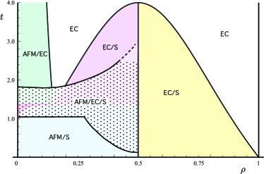
Figure 12: The $T=0$ phase diagram of the exciton $t$-$J\,$model for $J_{\perp}=0.02$, $J_{\parallel}=0.125$ and $V=2$. The parameters $t$ and $\rho$ denote the exciton hopping amplitude and concentration, respectively. The names of phases are the same as in Fig. 10: antiferromagnet (AFM), exciton condensate (EC) and solid (S). The slash, e.g., ’EC/S’, denotes phase separation. Adapted with permission of authors from Ref. Rademaker et al., 2013c. Copyrighted by the American Physical Society.

The small positive $J_{\perp}$ selects the spin-singlet condensate which is characterised by spontaneous coherence between the $|00\rangle$ and $|\emptyset\rangle$ states. The mean-field ground state can be written as ${|\Psi\rangle=\Pi_{i}(\sqrt{\rho}h_{i}^{\dagger}+\sqrt{1-\rho}s_{i}^{\dagger})|\Omega\rangle}$. An interesting consequence of the singlet condensation is an enhanced propagation of spin excitations (triplons). The authors of Refs. Rademaker et al., 2013a, c observed that the triplet excitations in the condensate of mobile excitons $t_{\text{ex}}\gg J_{\parallel}$ propagate faster that in the quantum paramagnet. Surprisingly, they found the effective triplon hopping scales with the density of the condensate $\rho_{\text{SF}}=\sqrt{\rho(1-\rho)}$ rather than the exciton density $\rho$.

III.4 Weak coupling

In the weak-coupling (BCS) limit the formation of excitons and their condensation take place at the same temperature. The physics of the system in this limit can be described by approaches such as Hartree-Fock approximation and RPA. The key feature of the weak-coupling theories is that EC instability is driven by nesting between the Fermi surface sheets formed by the valence and conduction bands. The lack of perfect nesting in real materials is likely one of the reasons why EC is rarely found in nature. The weak-coupling theory of the excitonic condensation in systems with equal concentration of holes and electrons was developed in 1960’s Keldysh and Kopaev (1965); des Cloizeaux (1965) and summarised in the review articles of Halperin and Rice Halperin and Rice (1968b, a). The pairing glue considered in the weakly-coupled semi-metals or semiconductors comes from the long-range part of the Coulomb interaction. The exchange part of the long-range Coulomb interaction is small, i.e. similar to the choice $J,J^{\prime}\approx 0$ in (7), and one has to consider both spin-singlet and spin-triplet pairing. Halperin and Rice Halperin and Rice (1968a) classified the possible excitonic condensates in systems with single Fermi surface sheet per band into the charge-density wave (real singlet), charge-current-density wave (imaginary singlet), spin-density wave (real triplet), spin-current-density wave (imaginary triplet) type . In case that there are multiple Fermi surface sheets related by point-group symmetries, e.g., as in hexaborides, a more complex symmetry classification is necessary Balents and Varma (2000); Murakami et al. (2002). The classification of Ref. Halperin and Rice, 1968a includes only the non-magnetic polar EC states. In mid 1970’s Volkov and collaborators showed that in a doped material with unequal number of electrons and holes ferromagnetic EC state develops characterised by simultaneous presence of finite singlet and triplet components  Volkov and Kopaev (1973); Volkov, Kopaev, and Rusinov (1975); Volkov, Rusinov, and Timerov (1976).

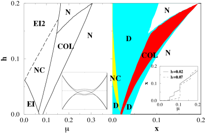
Figure 13: The mean-field phase diagram of doped 2BHM as a function of external field $\mathbf{h}$ and the chemical potential $\mu$ (left) and as a function of doping $x$ (right). The solid lines in the left panel mark first-order transitions. The light blue areas (marked D) in the right panel represent phase coexistence regions. The meaning of the different phases is described in the text. Adapted with permission of authors from Ref. Bascones, Burkov, and MacDonald, 2002. Copyrighted by the American Physical Society.

We briefly review the mean-field (Hartree-Fock) theory of (7) and consider the simplest case of uniform EC order ($t_{a}t_{b}<0$). The mean-field Hamiltonian that allows polar as well as ferromagnetic EC order reads

$$\begin{split}H&=\sum_{\mathbf{k},\sigma\sigma^{\prime}}\left(\epsilon_{\mathbf{k}a}\delta_{\sigma\sigma^{\prime}}-\mathbf{h}_{a}\cdot\bm{\tau}_{\sigma\sigma^{\prime}}\right)a^{\dagger}_{\mathbf{k}\sigma}a^{\phantom{\dagger}}_{\mathbf{k}\sigma^{\prime}}\\ &+\sum_{\mathbf{k},\sigma\sigma^{\prime}}\left(\epsilon_{\mathbf{k}b}\delta_{\sigma\sigma^{\prime}}-\mathbf{h}_{b}\cdot\bm{\tau}_{\sigma\sigma^{\prime}}\right)b^{\dagger}_{\mathbf{k}\sigma}b^{\phantom{\dagger}}_{\mathbf{k}\sigma^{\prime}}\\ &-\sum_{\mathbf{k},\sigma\sigma^{\prime}}\left(\left(\Delta_{s}\delta_{\sigma\sigma^{\prime}}+\bm{\Delta}_{t}\cdot\bm{\tau}_{\sigma\sigma^{\prime}}\right)b^{\dagger}_{\mathbf{k}\sigma}a^{\phantom{\dagger}}_{\mathbf{k}\sigma^{\prime}}+H.c.\right).\end{split}$$ (27)

Here, $a^{\phantom{\dagger}}_{\mathbf{k}\sigma},b^{\phantom{\dagger}}_{\mathbf{k}\sigma}$ are Fourier transforms of $a^{\phantom{\dagger}}_{i\sigma},b^{\phantom{\dagger}}_{i\sigma}$, respectively. The crystal-field splitting $\Delta$ as well as the spin-independent part of the self-energy are absorbed in band dispersions $\epsilon_{\mathbf{k}a},\epsilon_{\mathbf{k}b}$. In the following discussion we will assume $a$ to form the conduction band and $b$ to form the valence band. The Weiss fields $\mathbf{h}_{a},\mathbf{h}_{b},\Delta_{s},\bm{\Delta}_{t}$ are given by

$$\begin{split}\mathbf{h}_{a}=\mathbf{h}+\frac{U}{2N}\sum_{\mathbf{k},\sigma\sigma^{\prime}}\langle a^{\dagger}_{\mathbf{k}\sigma}a^{\phantom{\dagger}}_{\mathbf{k}\sigma^{\prime}}\rangle\bm{\tau}_{\sigma\sigma^{\prime}}\\ \Delta_{s}=\frac{U^{\prime}}{2N}\sum_{\mathbf{k},\sigma\sigma^{\prime}}\langle a^{\dagger}_{\mathbf{k}\sigma}b^{\phantom{\dagger}}_{\mathbf{k}\sigma^{\prime}}\rangle\delta_{\sigma\sigma^{\prime}}\\ \bm{\Delta}_{t}=\frac{U^{\prime}}{2N}\sum_{\mathbf{k},\sigma\sigma^{\prime}}\langle a^{\dagger}_{\mathbf{k}\sigma}b^{\phantom{\dagger}}_{\mathbf{k}\sigma^{\prime}}\rangle\bm{\tau}_{\sigma\sigma^{\prime}},\\ \end{split}$$ (28)

where $\mathbf{h}$ is the external magnetic field (acting on spin only). The field $\mathbf{h}_{b}$ is defined as $\mathbf{h}_{a}$ with the orbital flavour replaced. Note that for model (7) with local interactions ${(\Delta_{s},\bm{\Delta}_{t})=U^{\prime}(\phi_{s},\bm{\phi}_{t})}$, where $\phi_{s}$, $\bm{\phi}_{t}$ are the local order parameters. The generalisation to models with non-local interaction, which leads to $\mathbf{k}$-dependent Weiss fields, is straightforward and can be found in the literature.

Bascones et al. Bascones, Burkov, and MacDonald (2002) studied model (27) as a function of doping and external field $\mathbf{h}$ at $T=0$. The phase diagram, shown in Fig. 13, contains four phases: the normal phase (N), polar excitonic insulator (EI) phase and two metallic FMEC phases called NC and COL in Ref. Bascones, Burkov, and MacDonald, 2002. To illuminate the nature of these phases it is helpful to introduce $\Delta_{\sigma\sigma^{\prime}}=\tfrac{1}{2}(\Delta_{s}\delta_{\sigma\sigma^{\prime}}+\bm{\Delta}_{t}\cdot\bm{\tau}_{\sigma\sigma^{\prime}})$.

In the zero-field EI phase, the singlet and triplet EC orders are degenerate. A finite field $\mathbf{h}$, assuming $\mathbf{h}=h_{z}\hat{\mathbf{z}}$ and $h_{z}>0$ in the following, lifts the degeneracy. The undoped system selects a triplet state with $\Delta_{\uparrow\uparrow}=\Delta_{\downarrow\downarrow}=0$ and $|\Delta_{\uparrow\downarrow}|>|\Delta_{\downarrow\uparrow}|$. For sufficiently large $h_{z}$ the system enters the EI2 phase of Fig. 13 with $\Delta_{\downarrow\uparrow}=0$. Upon doping two distinct FMEC phases are found. In the NC the only non-zero element of the oder parameter is $\Delta_{\uparrow\downarrow}\neq 0$. The EI2 and NC phases are distinguished by presence of a $\mathbf{h}$-dependent gap between the uncondensed $a_{\downarrow}$ and $b_{\uparrow}$ bands. The order parameter in the NC phase is purely spin-triplet and the phase coincides with the FMEC phase of $S=1$ bosons in the strong-coupling limit. In the COL phase, the only non-zero element of $\Delta_{\sigma\sigma^{\prime}}$ is $\Delta_{\downarrow\downarrow}\neq 0$. In this phase, predicted by Volkov et al. Volkov, Kopaev, and Rusinov (1975) the singlet and triplet order parameters mix with equal weight ($\Delta_{s}=-\Delta^{z}_{t}$).

The $\mathbf{h}=0$ spin-wave spectrum of the COL state for a general chemical potential $\mu$ is characterised by two gapless modes with a quadratic dispersion at small $|\mathbf{q}|$ and an additional soft but gapped mode Bascones, Burkov, and MacDonald (2002). At a special value of $\mu$ the soft mode becomes gapless and the spectrum has one quadratic and two linear modes. The mean-field phase diagram and magnetic excitations of the polar EI phase in the undoped model were studied by Brydon and Timm Brydon and Timm (2009a) and Zocher et at. Zocher, Timm, and Brydon (2011) using RPA. They observed acoustic-like modes with linear dispersion at small $|\mathbf{q}|$ predicted by Kozlov and Maksimov Kozlov and Maksimov (1966) and Jérome et al. Jérome, Rice, and Kohn (1967).

Moving away from the strong-coupling limit the separation of energy scales of exciton formation and exciton condensation is progressively less well defined and eventually these scales are not separated at all. As in the spinless case of EFKM, EC exists also at weak-coupling and one can follow the BEC-BCS crossover as the interaction strength is lowered. The weak-coupling methods, such as Hartree-Fock approximation and RPA, were applied to study the EC in its early days and are summarised in the review article of Halperin and Rice Halperin and Rice (1968b, a).

III.5 Intermediate coupling

Investigations of systems with intermediate-coupling strength are notoriously difficult due to the lack of small parameters. The general approaches to this problem include numerical simulations of finite systems such as exact diagonalisation or quantum Monte-Carlo (QMC) methods, large-N expansions, and embedded impurity or imbedded cluster methods such as dynamical mean-field theory Georges et al. (1996) (DMFT), variational cluster approximation Potthoff, Aichhorn, and Dahnken (2003), dynamical cluster approximation or cluster DMFT Maier et al. (2005). A major obstacle in simulation of ordering phenomena with finite-system methods is the necessity of scaling analysis, i.e., the cluster size must be large enough to show the ’diverging’ correlation length. Monte-Carlo simulations on large clusters are available for many bosonic and spin systems, but usually not for fermions. Rademaker et al Rademaker et al. (2013b) applied the determinant Monte-Carlo method to bi-layer Hubbard model and were able to demonstrate an enhanced response to the excitonic pairing field, but could not reach temperatures below $T_{c}$. Besides the Green’s function QMC methods for calculation of correlation functions, wave function QMC approaches can be applied to variational search for ground states. While we are not aware of variational QMC studies of excitonic condensation in Hubbard-type lattice models, variational QMC has been used to study the corresponding continuum problem Zhu, Hybertsen, and Littlewood (1996).

The DMFT methods have been very valuable for investigation of Hubbard model and its multi-band generalisations in the past two decades. However, most applications of DMFT so far focused on one-particle quantities and normal (paramagnetic) phase. With an exception of a multi-band study of Ref. Park, Haule, and Kotliar, 2011, linear response calculations needed to identify instabilities have been so far limited to simple one- Jarrell (1992) and two-band models Jarrell, Akhlaghpour, and Pruschke (1993); Ulmke, Janiš, and Vollhardt (1995); Kuneš and Augustinský (2014a). Recent DMFT investigations of ordered phases in models as simple as 2BHM uncovered a rich physics. Capone et al. Capone et al. (2002, 2004), Koga and Werner Koga and Werner (2015) and Vanhala at al. Vanhala et al. (2014) found various forms of superconductivity in 2BHM at half-filling. Recently, dynamical cluster approximation was also applied to study excitonic condensation. Vanhala et al. (2014)

III.5.1 Half filling

Kuneš and collaborators studied 2BHM (7) in the vicinity of spin-state transition, see also Fig. 7, using DMFT Kuneš and Křápek (2011); Kuneš and Augustinský (2014a, b); Kuneš (2014) for 2BHM (7) with $V_{ab},V_{ba},J^{\prime}=0$ and density-density interaction. In Ref. Kuneš and Křápek (2011), they reported observation of the solid phase for the case of strongly asymmetric bands $|t_{a}|\gg|t_{b}|$. The normal/solid phase boundary qualitatively agrees with strong-coupling BEG model. In particular, the re-entrant transition as a function of temperature for large $\Delta$ has been found. In Ref. Kuneš and Augustinský, 2014a, an unbiased linear response DMFT approach Kuneš (2011) was used to probe stability of the normal phase. Two types of instabilities were found, an instability towards the solid and an instability towards the excitonic condensate. This situation resembles EFKM. Indeed, the physics behind formation of the solid and the superfluid phases in the strong-coupling limits of EFKM and 2BHM is similar. As in EFKM, the excitonic instability in 2BHM extends to the weak-coupling limit. This is not so for the solid phase. In the weak-coupling limit, the instability towards solid either does not exist at all or is weaker than the antiferromagnetic instability.

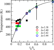
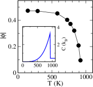
Figure 14: Left: The instability temperature of the normal phase for various band asymmetries $t_{b}/t_{a}$ and crystal-fields $\Delta$. The squares mark the divergence of the orbital susceptibility (instability towards the solid order), the circles correspond to the divergence of the excitonic susceptibility. The sum $t_{a}^{2}+t_{b}^{2}$ was kept fixed. Data taken from Ref. Kuneš and Augustinský, 2014a. Right: The magnitude of the order parameter $|\phi(T)|$ along the trajectory marked by arrow in the left panel. The specific heat per site along the same line is shown in the Inset. Adapted from Ref. Kuneš and Augustinský, 2014b. Copyrighted by the American Physical Society.

The basic physical properties of the excitonic phase were studied in Ref. Kuneš and Augustinský, 2014b. In Fig. 14, we show a typical $T$-dependence of the magnitude of the order parameter $|\phi|$. The systems selected a polar EC state, $\bar{\bm{\phi}}_{i}\wedge\bm{\phi}_{i}=0$,  which agrees with the antiferromagnetic nn exchange expected in the the strong-coupling limit (15). The shape of $|\phi(T)|$ is consistent with the mean-field $(1-T/T_{c})^{1/2}$ dependence, expected for DMFT method. As in the weak-coupling limit, the excitonic condensation leads to opening of a charge gap and appearance of Hebel-Slichter peaks in the one-particle spectra, see Fig. 15. This behaviour reflects the formal analogy to an $s$-wave superconductor discussed in Sec. II.

This analogy however, does not extend to the electromagnetic properties of the condensate. The neutral exciton condensate does not contribute to the charge transport, which is facilitated by the quasi-particle excitations. In Fig. 15 we show the optical conductivity and $dc$ resistivity at various temperatures. The opening of the charge gap leads to an optical gap and exponential increase of the resistivity below $T_{c}$.

Finally, we discuss the spin susceptibility $\chi_{s}^{zz}$, shown in Fig. 16. While the normal-phase susceptibility exhibits Curie-Weiss behaviour, the susceptibility of the polar EC phase appears $T$-independent. This observation holds within the numerical accuracy for the uniform susceptibility and approximately also for the local susceptibility. This behaviour can be understood from a single atom picture. In the normal phase, the system is locally in a statistical mixture of the LS ground state and thermally populated HS multiplet. This leads to Curie-Weiss susceptibility and a vanishing of the spin gap. In the polar EC phase, the Weiss field mixes the LS and HS states and opens a gap of the order $U^{\prime}\phi/2\gg T$ between the local ground state and the excited states. The local ground state is a superposition of the form $\alpha|\emptyset\rangle+\beta(|-1\rangle+|1\rangle)$. The spin susceptibility has $T$-independent van Vleck character and a finite spin gap appears, Fig. 16.

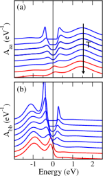
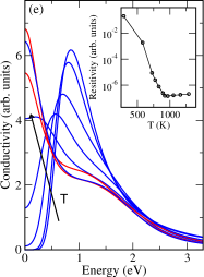
Figure 15: Left: The evolution of the one-particle spectral functions (diagonal elements) with temperature along the line marked in Fig. 14a. The spectra are taken at $T$=1160, 968, 921, 892, 829, 725, 580, and 290 K. Right: The corresponding optical conductivity. The Inset shows the $T$-dependence of the $dc$ resistivity. Adapted from Ref. Kuneš and Augustinský, 2014b. Copyrighted by the American Physical Society.

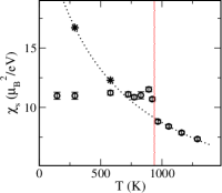
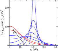
Figure 16: Left: The static uniform spin susceptibility $\chi_{s}$ (circles with error bars) along the line marked in Fig. 14a. The stars and dotted line indicate $\chi_{s}(T)$ for the system constrained to the normal state. The red vertical line marks the EC transition. Adapted from Ref. Kuneš and Augustinský, 2014b. Copyrighted by the American Physical Society. Right: The imaginary part of the local dynamic susceptibility $\chi_{\text{loc}}(\omega)$ at various temperatures across the EC transition Kuneš .

Kaneko et al. Kaneko, Seki, and Ohta (2012) used variational cluster approximation to study the spin-triplet EC in 2BHM without Hund’s coupling ($J,J^{\prime}=0$) and with symmetric bands $t_{a}=t_{b}$ for a broad range of interaction parameters. Similar to the strong-coupling phase diagram Fig. 10 the authors of Ref. Kaneko, Seki, and Ohta, 2012 found continuous transition between the EC and normal state (band insulator), and a first-order transition between the EC and AFM phases as shown in Fig. 17. In Ref. Kaneko and Ohta, 2014, Kaneko and Ohta extended the study to include the Hund’s coupling, which confirmed that $J<0$ favours the spin-singlet charge-density-wave state, while $J>0$ selects the spin-triplet spin-density-wave state Halperin and Rice (1968a); Buker (1981).

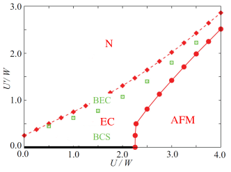
Figure 17: The $T=0$ phase diagram of 2BHM on a square lattice for $t_{a}=t_{b}=1$ ($W=4$), $V_{ab},V_{ba},J,J^{\prime}=0$, $\Delta=6$ obtained with variational cluster approximation. The transition between the band insulator (N) and the EC phase is continuous, the EC/AFM phase transition is of the first order. The thick black line for $U^{\prime}=0$ marks a paramagnetic metal. Adapted with permission of authors from Ref. Kaneko, Seki, and Ohta, 2012. Copyrighted by the American Physical Society.

III.5.2 Doping

The weak-coupling theory of doped excitonic insulator was developed by Volkov and collaborators Volkov and Kopaev (1973); Volkov, Kopaev, and Rusinov (1975); Volkov, Rusinov, and Timerov (1976) for systems without Hund’s coupling. They showed that such systems tend to develop ferromagnetic order due to simultaneous appearance of the spin-singlet and spin-triplet order. In Sec. III.4, we have reviewed the application of the weak-coupling approach by Bascones et al. Bascones, Burkov, and MacDonald (2002). Besides finding Volkov’s ferromagnetic phase (COL) the authors of Ref. Bascones, Burkov, and MacDonald, 2002 found also a spin-triplet phase (NC) induced by an external magnetic field. The possibility of the triplet ferromagnetism was discussed also by Balents Balents (2000) who considered the effect of doping in a strong coupling limit on a qualitative level.

Kuneš Kuneš (2014) used DMFT to study the effect of doping in 2BHM with strong Hund’s coupling, which limits the possible EC order to spin triplet. The phase diagram, shown in Fig. 18, contains the normal phase (open circles) and three excitonic phases. The polar phase (red), discussed in preceding section at half-filling, extends to finite doping levels. It is distinguished from the other two phases by absence of ordered spin moment. The relation ${\bm{\phi}^{*}\wedge\bm{\phi}=0}$ implies that $\bm{\phi}$ can be factorised to a real vector and a phase factor. The arbitrariness of the phase factor is connected to the absence of the cross- and pair-hopping in the studied model. The polar phase is equivalent to the EI phase in Fig. 13.

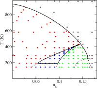
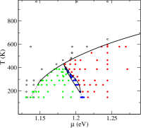
Figure 18: Phase diagram of 2BHM with hole-doping (counted from half-filled case) (left) and chemical potential (right) on the horizontal axis. Solid lines mark continuous transitions, while dashes lines mark the first order transitions (right) or boundaries to the phase separation regime (left). The coloured dots represent the actual numerical calculations. The red colour marks the polar EC phase, the blue and green colour mark the FMEC phase. The blue and green phases are distinct when the cross-hopping in (7) is strictly zero. Adapted from Ref. Kuneš, 2014. Copyrighted by the American Physical Society.

At higher doping levels and lower temperatures the system enters the FMEC phase with finite magnetisation ${\mathbf{m}\sim i(\bm{\phi}^{*}\wedge\bm{\phi})\neq 0}$. The transition between polar and ferromagnetic phases proceeds via an intermediate phase (blue), which is distinguished from the FMEC only in absence of cross- and pair-hopping Kuneš (2014). The FMEC phase is equivalent to the COL phase of Ref. Bascones, Burkov, and MacDonald, 2002 (Fig. 13). Similar to the $T=0$ phase diagram of Ref. Bascones, Burkov, and MacDonald, 2002, first-order transitions and phase separation is found at low temperatures. It is not clear from the numerical data whether a $T=0$ polar phase exists at finite doping. At the moment we can only speculate that the antiferromagnetic nn coupling provides a means to stabilise it. A peculiar feature of the FMEC is the $T$-dependence of the magnetisation in the vicinity of the continuous transition to the normal state, which follows the linear ${1-T/T_{c}}$ dependence. This behaviour is a consequence of the quadratic dependence of magnetisation on the EC order parameter ${\mathbf{m}\sim i(\bm{\phi}^{*}\wedge\bm{\phi})}$.

Finally, we briefly discuss the effect of finite cross- and/or pair-hopping, which break the charge conservation per orbital flavour. As a result the phase factor in the polar EC phase is fixed and the system selects either the spin-density-wave or spin-charge-density-wave order. It is also possible that both types of order are realised in parts of the phase diagram. Another consequence of finite cross-/pair- hopping will be the absence of a continuous normal to FMEC transition. The FMEC state is selected by terms of the order $\phi^{4}$ in the Ginzburg-Landau functional and a continuous transition is only possible if the second order terms do not depend on the phase of $\phi$. Finite cross-/pair- hopping removes this degeneracy. For weak cross hopping one can expect a small wedge of polar EC phase separating the normal and FMEC phases. The first-order normal/FMEC transitions are still possible.

IV Multi-orbital Hubbard model

Little has been done in generalisation of the physics of Sec. III to systems with more than two orbitals per atom. Kuneš and Augustinský Kuneš and Augustinský (2014b) used Hatree-Fock (LDA+U) approach to study EC in quasi-cubic perovskite with nominally 6 electrons in the $d$ shell. Let us demonstrate the new features on 5-orbital model describing the $d$-orbital atoms on a cubic lattice. The basic setting of such system is similar to half-filled two-orbital model. The crystal-field splits the $d$ orbitals into threefold degenerate $t_{2g}$ and twofold degenerate $e_{g}$ states. With 6 electrons per atom the lower $t_{2g}$ levels are filled and the upper $e_{g}$ levels are empty. An exciton is formed by moving an electron from a $t_{2g}$ orbital to an $e_{g}$ orbital on the same atom. Unlike 2BHM with only one possible orbital structure of an exciton, in the $d$-atom there are six possible orbital combinations. The cubic symmetry distinguishes the orbital symmetries of an exciton into two 3-dimensional irreducible representations $T_{1g}$ and $T_{2g}$. Considering the geometry of these two excitons Kuneš and Augustinský (2014b) one can infer that $T_{1g}$ excitons are more tightly bound and substantially more mobile that the $T_{2g}$ ones. Therefore only the $T_{1g}$ excitons need to be considered as candidates for condensation. The three-fold orbital degeneracy of the $T_{1g}$-excitons adds to the $S=1$ spin degeneracy making the order parameter a more complex object. It can be arranged to a tensorial form of a $3\times 3$ matrix $\phi^{\alpha}_{\beta}$, where the $\alpha$ indexes the spin and $\beta$ the orbital components. $\phi^{\alpha}_{\beta}$ thus transforms as a vector under the $SO(3)$ rotations in the spin space and as a pseudo vector ($T_{1g}$ representation) under the discrete symmetry operations of the cubic point group. The explicit expression for $\phi^{\alpha}_{\beta}$ in terms of the on-site occupation matrix can be found in the supplementary material of Ref. Kuneš and Augustinský, 2014b. The structure of the order parameter resembles of superfluid ³He Vollhardt and Wölfle (2013) and one can use the group theoretical methods applied there to analyse the possible EC phases Bruder and Vollhardt (1986). More complex structure of the order parameter allows for existence of numerous distinct phases.

Another important difference to 2BHM concerns the hard-core constraint imposed in the excitons in the strong coupling limit. While in the case of 2BHM there cannot be more than one exciton on a given atom, in the 5-orbital model the hard-core constraint is less restrictive. There cannot be more than one exciton of a given orbital flavour on atom, but it is possible that two excitons with different orbital flavours meet. In the cobaltites terminology a single exciton on atom represents the intermediate spin $S=1$ state, while the $S=2$ high-spin state can be viewed as a bi-exciton. The fact that the site energy of the high-spin state is lower than of the intermediate-spin state Tanabe and Sugano (1954) is then expressed as an attraction between excitons of different orbital flavour and parallel spins. Bosonic models with infinite intra-species, but finite inter-species interaction have been studied for two species (spinless) bosons Altman et al. (2003); Kuklov and Svistunov (2003); Trousselet, Rueda-Fonseca, and Ralko (2014); Lv, Chen, and Deng (2014) and shown to exhibit phases which are not allowed with inter-species hard-core constraint.

V Materials

V.1 Bulk materials

There have been numerous proposals of materials to exhibit excitonic condensation, but very few realisations of EC were actually documented. The early candidates for excitonic condensation, which followed the weak-coupling picture of proximity to semimetal–semiconductor transition, included the group V semimetals (Bi, Sb, As) and divalent metals (Ca, Sr, Yb), possibly under pressure Jérome, Rice, and Kohn (1967). However, the search for signatures of EC in these materials was not successful.

Wachter and collaborators Neuenschwander and Wachter (1990); Bucher, Steiner, and Wachter (1991); Wachter (2001); Wachter, Bucher, and Malar (2004) reported observation of EC in TmSe_0.45Te_0.55 under pressure. While they did not see a sharp thermodynamic transition, they argued that the observed anomalies are consistent with a ’transition’ in weak (pairing) field. Wakisaka et al. Wakisaka et al. (2009) interpreted their photoemission data on Ta₂NiSe₅ in terms of exciton condensation Kaneko, Seki, and Ohta (2012); Kaneko et al. (2013b); Seki et al. (2014). Also the lattice distortion and photoemission spectra of a layer compound 1$T$-TiSe₂ have been interpreted in terms of charge-density-wave type exciton condensation and described with the weak-coupling theory Cercellier et al. (2007); Monney et al. (2009, 2010, 2011).

While the previous examples involved cases of spin-singlet condensation, in the following we will discuss excitonic magnetism. In 1999 Young et al. Young et al. (1999) reported observation of 600 K ferromagnetism in La_0.005Ca_0.995B₆. Ferromagnetism in a slightly doped semiconductor lead several groups to generalise the weak-coupling theory of excitonic ferromagnetism pioneered by Volkov and collaborators Volkov and Kopaev (1973); Volkov, Kopaev, and Rusinov (1975); Volkov, Rusinov, and Timerov (1976) to the case of multiple Fermi surface sheets Zhitomirsky, Rice, and Anisimov (1991); Balents and Varma (2000); Veillette and Balents (2001); Barzykin and Gor’kov (2000); Murakami et al. (2002). Subsequent investigations showed, nevertheless, that the band gap in parent compound CaB₆ is $\approx 1$ eV Denlinger et al. (2002) and thus inconsistent with the EC scenario. It is now generally accepted that the ferromagnetism in La_xCa_1-xB₆ arises from defects rather that doping.

Another group of materials where the EC concept found its use are iron pnictides Kamihara et al. (2008); Stewart (2011). The physics of these materials is governed by nesting between several Fermi surface sheets formed by bands of different orbital characters Graser et al. (2010). Several groups studied a simplified two-orbital model Han, Chen, and Wang (2008); Chubukov, Efremov, and Eremin (2008); Brydon and Timm (2009b, a) and its multi-orbital extensions Knolle et al. (2010); Eremin and Chubukov (2010) using weak-coupling approaches, and observed a spin-density-wave order with a periodicity given by the nesting vector. Arising from nesting between bands that mix several orbital characters, the corresponding Weiss field in general couples all possible orbital combinations. However, since the nested patches of the Femi surface have different dominant orbital characters a large part of the condensation energy comes from orbital off-diagonal pairing, which produces local magnetic multipoles but no local moments (polar EC state). The generally present, but small, orbital diagonal contributions than give rise to the apparently small ordered moments. A first principles calculation of ordered state supporting this picture was done by Crincchio et al. Cricchio, Grånäs, and Nordström (2010).

Kuneš and Augustinský Kuneš and Augustinský (2014a) proposed that a transition observed in some materials of Pr_xCa_1-xCoO₃ (PCCO) family Tsubouchi et al. (2002, 2004); Hejtmánek et al. (2010, 2013) can be understood as an excitonic condensation. Materials from this family exhibit a phase transition with $T_{c}$ as high as 130 K which is characterised by sharp peak in the specific heat, transition from high-$T$ metal to a low-$T$ insulator, disappearance of Co local moment response and simultaneous Pr³⁺ $\rightarrow$ Pr⁴⁺ valence transition. A puzzling feature of the low temperature phase is the breaking of time reversal symmetry (in absence of ordered moments) evidenced by Schottky anomaly associated with splitting of the Pr⁴⁺ Kramer’s ground state. The transition to a spin-density-wave EC state provides a comprehensive explanation of these observations and the EC ground state is obtained with Hartree-Fock-type LDA+U calculations.

Another class of the materials with potential to exhibit the exciton condensation was proposed by Khaliullin Khaliullin (2013); Akbari and Khaliullin (2014). He considered a strong-coupling model of a $d$-electron material with cubic crystal field, strong spin-orbit coupling and an average $d$ occupancy of four electrons per atom. A scenario possibly realised in materials with Re³⁺, Ru⁴⁺, Os⁴⁺, or Ir⁵⁺ ions. The large crystal field restricts the low energy physics to the space spanned by $t_{2g}$ states. Now the spin-orbit coupling plays the role of $\Delta$ in (7) competing with the Hund’s coupling $J$. Sufficiently strong spin-orbit coupling renders the single-ion ground state a singlet $\tilde{S}=0$  and the first excited state a triplet $\tilde{S}=1$. The perturbative treatment of nn hopping results in the model similar to (17). There is, however, one important difference between (17) and the Khaliullin’s model formulated in terms of pseudospin $\tilde{\mathbf{S}}$. The real spin $\mathbf{S}$ is decoupled from the lattice and thus (17) is invariant under the $SO(3)$ spin spin rotations, in particular the hopping $K_{\perp}$ is spin independent. The pseudospin $\tilde{\mathbf{S}}$ represents a spin-orbital object, which is coupled to the lattice and thus the model cannot be invariant under continuous pseudospin rotations. This is reflected in the hopping amplitudes being $\tilde{S}$-dependent, i.e., the hopping containing terms known from Kitaev model Kitaev (2006).

Finally, the possibility of exciton condensation in layered cuprates bri (2005) and oxide heterostructures Millis and Schlom (2010) was discussed by several authors, but has not been realised so far.

V.2 Bi-layer structures

A major direction in the research of exciton condensation are bi-layer structures Lozovik and Yudson (1975). The basic idea is that a bi-layer with negligible inter-layer tunnelling provides a system where two orbital flavours are to high accuracy independently conserved. Exciton condensation takes place under suitable conditions including small inter-layer distance, so that inter-layer electron-electron interaction is sufficiently strong, large enough intra-layer electron mobility, so that sufficiently high $T_{c}$ can be achieved, and a matching doping, such that the electron concentration in one layer closely matches the hole concentration in the other layer. Two types of structures have been studied. 2D quantum well systems in perpendicular magnetic field. The idea here is to use the formation of Landau levels and, in particular, the dependence of the number of quantum states per Landau level on the magnetic field as a means to achieve the desired electron and holes concentrations. The exciton condensation in these systems was evidenced by enhanced inter-layer tunnelling Spielman et al. (2000) or vanishing Hall conductivity Eisenstein and MacDonald (2004). For a review of experimental challenges probing exciton condensation in bi-layers we refer the reader to specialised literature Das Gupta et al. (2011).

Another bi-layer system that has been intensely studied is the system of two graphene layers separated with a dielectric where EC was predicted to take place at room temperature Min et al. (2008). The important and much debated issue here is the screening of the inter-layer interaction Kharitonov and Efetov (2008). The system therefore cannot be described with a simple Hubbard type model for the strongly correlated electrons. For a review of the physics of electron-electron interaction in graphene structures we refer the reader to a specialised literature Kotov et al. (2012).

VI Outlook

Analogy to superconductivity has been the traditional driving force of the field of exciton condensation. In particular, there was a considerable effort in realisation of supercurrents driven by the gradient of the condensate phase – a hallmark of superfluidity. There are two important conditions to realise a supercurrent. First, the phase invariance (conduction/valence charge conservation) in the normal phase. Second, the ability to contact separately the electron and the hole parts of the exciton. These conditions can be met in bi-layer systems, where the electrons and hole are spatially separated while maintaining sufficiently strong interaction. We find it, however, unlikely that similar situation can be realised in bulk materials. Already the first condition is bound to be violated by various one- and two-particle terms in the Hamiltonian as discussed previously. Instead of a superfluid with an arbitrary phase the system selects either charge(spin)-density-wave or charge(spin)-current-density-wave state Halperin and Rice (1968a) with a fixed phase. Omitting possible special points in the phase diagram where the symmetry may be enhanced, e.g., close to a second-order boundary between these phases the system will not exhibit a superfluid behaviour.

The main value of the concept of exciton condensation in bulk materials lies, in our opinion, in providing a comprehensive picture of potentially complex phase diagrams and understanding long-range orders that are not easy to detect because they do not lead to charge(spin)-density modulations on inter-atomic scale. Moreover, the geometrical form of the order parameter in EC system may non be as intuitive as for example magnetisation is systems with local moments. For example, exciton condensation in $s$-$p$ systems leads to formation of electric dipoles Batista (2002) or condensation in a system close to the spin-state transition gives rise to a magnetic multipole order Kuneš and Augustinský (2014a). There are other examples of orbital-off-diagonal orders, e.g. orbital currents in cuprates Varma (2006); Weber, Giamarchi, and Varma (2014); Bulut, Kampf, and Atkinson (2015), nematic order in iron pnictides Kasahara et al. (2012); Rosenthal et al. (2014); Fernandes, Chubukov, and Schmalian (2014), hidden order in URu₂Si₂ Mydosh and Oppeneer (2011) where we can only speculate that they may be viewed as a special example of the EC physics. It should be clear from this discussion that the concept of exciton condensation extended beyond the strict superfluid state is not sharply defined and, in particular, the weak-coupling borderline between exciton condensation and ’just a’ Fermi surface instability is quite fuzzy.

We see numerous open questions and possible directions of further investigation. In the two-band model, realisation of spin-current-density-wave phase and in general the phase diagram in the presence of cross-hopping are to be explored. The Weiss field in the spin-current-density-wave state can be viewed as a spontaneous spin-orbit coupling - a field that breaks the spin-rotational symmetry, but preserves the time reversal symmetry. Interaction between the exciton condensate and the lattice has attracted attention recently Zenker, Fehske, and Beck (2014). The multi-band systems with multiple orbital flavours of excitons are completely unexplored to our knowledge. A model that can shed some new light on the long standing problem of perovskite cobaltites.