Redshift-space distortions of galaxies, clusters and AGN

Abstract

Aims. Redshift-space clustering anisotropies caused by cosmic peculiar velocities provide a powerful probe to test the gravity theory on large scales. However, to extract unbiased physical constraints, the clustering pattern has to be modelled accurately, taking into account the effects of non-linear dynamics at small scales, and properly describing the link between the selected cosmic tracers and the underlying dark matter field.

Methods. We use a large hydrodynamic simulation to investigate how the systematic error on the linear growth rate, $f$, caused by model uncertainties, depends on sample selections and comoving scales. Specifically, we measure the redshift-space two-point correlation function of mock samples of galaxies, galaxy clusters and Active Galactic Nuclei, extracted from the Magneticum simulation, in the redshift range $0.2\leq z\leq 2$, and adopting different sample selections. We estimate $f\sigma_{8}$ by modelling both the monopole and the full two-dimensional anisotropic clustering, using the dispersion model.

Results. We find that the systematic error on $f\sigma_{8}$ depends significantly on the range of scales considered for the fit. If the latter is kept fixed, the error depends on both redshift and sample selection, due to the scale-dependent impact of non-linearities, if not properly modelled. On the other hand, we show that it is possible to get almost unbiased constraints on $f\sigma_{8}$ provided that the analysis is restricted to a proper range of scales, that depends non trivially on the properties of the sample. This can have a strong impact on multiple tracers analyses, and when combining catalogues selected at different redshifts.

1 Introduction

The dynamics of the Universe is shaped by the gravity force. The understanding of gravity is thus the key to unveil the nature of the Universe and its cosmological evolution. After almost one century from its original formulation, Einstein’s General Relativity (GR) is still the dominant theory to describe gravity. However, despite its lasting experimental successes, some fundamental open issues are motivating challenging efforts aimed at searching for possible expansions or radically alternative models (Amendola et al. 2013). First of all, GR is not a quantum field theory and cannot be reconciled with the principles of quantum mechanics. Secondly, an increasingly large amount of astronomical observations cannot be explained by GR and baryonic matter alone, requiring the introduction of a never observed form of dark matter (DM, Zwicky 1937). Finally, independent cosmological observations give indisputable evidences for an accelerated expansion of the Universe, requiring the introduction of another dark component, generally dubbed dark energy (DE), when interpreted in the GR framework (Riess et al. 1998; Perlmutter et al. 1999). Whether GR provides a reliable description of the large scale structure of the Universe, and thus the latter is dominated by unknown dark components, or, on the contrary, such a gravity theory has to be corrected, or even abandoned, is one of the key questions of modern physics and cosmology.

One of the most effective ways to test the gravity theory on large scales, that is where DM and DE arise, is to exploit the apparent anisotropies observed in galaxy maps, the so-called redshift-space distortions (RSD, Kaiser 1987; Hamilton 1998). Indeed, by modelling redshift-space clustering anisotropies it is possible to constrain the linear growth rate of cosmic structures, $f\equiv d\log\delta/d\log a$, where $a$ is the dimensionless scale factor and $\delta$ the linear fractional density perturbation, provided that the galaxy bias is known. The first RSD measurements were exploited primarily to estimate the mean matter density, $\Omega_{\rm M}$ , that can be derived directly from $f(z)$ when a gravity model is assumed (Peacock et al. 2001; Hawkins et al. 2003). Later on, Guzzo et al. (2008) and Zhang et al. (2008) showed that RSD can be effectively used to discriminate between DE and modified gravity scenarios. RSD thus started to be considered as a powerful probe of gravity, and several applications to galaxy redshift surveys followed rapidly, both in the local Universe and at larger redshifts, up to $z\sim 1$, such as 6dFGS (Beutler et al. 2012), SDSS (Samushia et al. 2012; Chuang & Wang 2013; Chuang et al. 2013), WiggleZ (Blake et al. 2012; Contreras et al. 2013), VIPERS (de la Torre et al. 2013), and BOSS (Tojeiro et al. 2012; Reid et al. 2012, 2014).

All the above measurements have been obtained from large galaxy redshift surveys. First tentative studies are starting to consider also different tracers, but results are still strongly affected by statistical uncertainties, due to the paucity of the catalogues used. Thanks to the wealth of observational data now available, or expected in the next future, for instance from the ESA Euclid mission (Laureijs et al. 2011), the NASA Wide Field Infrared Space Telescope (WFIRST) mission (Spergel et al. 2013), and the extended Roentgen Survey with an Imaging Telescope Array (eROSITA) satellite mission (Merloni et al. 2012), it will soon become possible to apply these methodologies on both cluster and Active Galactic Nuclei (AGN) catalogues. Galaxy clusters are the biggest collapsed structures in the Universe. They appear more strongly biased than galaxies, that is their clustering signal is higher. Moreover, they are relatively unaffected by non-linear dynamics on small scales. This could help in modelling redshift-space distortions in their clustering pattern, as the effect of small scale incoherent motions, that generate the so-called fingers-of-God pattern, is substantially less severe relative to the galaxy clustering case, improving also the cosmological constraints that can be extracted from baryon acoustic oscillations (Veropalumbo et al. 2014). The main drawback is the low density of galaxy cluster samples and the fact that these sources can be reliably detected only at relatively small redshifts. On the other hand, AGN can be detected up to very large distances. Powered by accreting supermassive black holes hosted at their centres, their extreme luminosities make them optimal tracers to investigate the largest scales of the Universe, and thus its cosmological evolution (see e.g. Marulli et al. 2008, 2009; Bonoli et al. 2009, and references therein).

The aim of this paper is to investigate the accuracy of the so-called dispersion model (that will be described in §3) as a function of comoving scales and sample selection. To achieve this goal, we exploit realistic mock samples of galaxies, galaxy clusters and AGN extracted from the Magneticum hydrodynamic simulation, at six snapshots in the range $0.2\leq z\leq 2$. We adopt a similar methodology as in Bianchi et al. (2012), though substantially extending that analysis. Specifically, i) in line with the majority of recent studies, we investigate the systematic errors of $f\sigma_{8}$, instead of $\beta$, ii) we consider different kinds of realistic mock tracers, instead of just DM haloes, iii) we analyse the dependency of the errors as a function of redshift, and iv) as a function of different sample selections. In agreement with previous investigations (see e.g. Bianchi et al. 2012; Mohammad et al. 2016), we find that the rough modelisation of non-linear dynamics provided by the dispersion model introduces systematic errors on $f\sigma_{8}$ measurements, that depend non trivially on the redshift and bias of the tracers. On the other hand, as we will demonstrate, it is possible to substantially reduce the systematic errors on $f\sigma_{8}$ provided that the fit is restricted in a proper range of scales, that depends on sample selection. An alternative investigation of the impact of the galaxy sample selection function on the ability to test GR with RSD has been carried out recently by Hearin (2015), analysing the small-scale effects of the assembly bias in velocity space.

The software that we implemented to perform all the analyses presented in this paper can be freely downloaded at this link: http://apps.difa.unibo.it/files/people/federico.marulli3/. It consists of a set of C++ libraries that can be used for several astronomical calculations, in particular to measure the two-point correlation function and to model RSD (CosmoBolognaLib, Marulli et al. 2016). We also provide the full documentation for these libraries, and some example codes that explain how to use them.

The paper is organised as follows. In §2 we describe the Magneticum simulation used to construct mock samples of galaxies, clusters and AGN, whose main properties are reported in Appendix A. In §3 and §4 we present the formalism used to model RSD and to measure the two-point correlation function in redshift-space mock catalogues, respectively. The results of our analyses are presented in §5. In §7 we summarise our conclusions. Finally, in the appendices B and C we discuss the tests performed to investigate the robustness of the methods applied in our analysis.

2 The Magneticum simulation

The most direct way to investigate systematic errors on linear growth rate measurements from RSD is to exploit large numerical simulations, and to apply on them the same methodologies used for real data. As our goal is to study the effects of different sample selections, we make use of realistic mock catalogues of different cosmic tracers. Specifically, we analyse galaxy, cluster and AGN mock catalogues extracted from the hydrodynamic Magneticum simulation (Dolag et al. in preparation).

This simulation is based on the parallel cosmological TreePM-SPH code P-GADGET3 (Springel 2005). The code uses an entropy-conserving formulation of smoothed-particle hydrodynamics (SPH) (Springel & Hernquist 2002) and follows the gas using a low-viscosity SPH scheme to properly track turbulence (Dolag et al. 2005). It also allows a treatment of radiative cooling, heating from a uniform time-dependent ultraviolet background and star formation with the associated feedback processes. The latter is based on a sub-resolution model for the multiphase structure of the interstellar medium (ISM) (Springel & Hernquist 2003a).

Radiative cooling rates are computed by following the same procedure presented by Wiersma et al. (2009). We account for the presence of the cosmic microwave background and of ultraviolet/X-ray background radiation from quasars and galaxies, as computed by Haardt & Madau (2001). The contributions to cooling from each one of the following 11 elements, H, He, C, N, O, Ne, Mg, Si, S, Ca, Fe, have been pre-computed using the publicly available CLOUDY photoionization code (Ferland et al. 1998) for an optically thin gas in photoionization equilibrium.

In the multiphase model for star-formation (Springel & Hernquist 2003b), the ISM is treated as a two-phase medium where clouds of cold gas form from cooling of hot gas and are embedded in the hot gas phase assuming pressure equilibrium whenever gas particles are above a given threshold density. The hot gas within the multiphase model is heated by supernovae and can evaporate the cold clouds. A certain fraction of massive stars (10 per cent) is assumed to explode as supernovae type II (SNII). The released energy by SNII ($10^{51}$ erg) is modelled to trigger galactic winds with a mass loading rate being proportional to the star formation rate to obtain a resulting wind velocity of $v_{\mathrm{wind}}=350$ km/s. Our simulation also includes a detailed model of chemical evolution according to Tornatore et al. (2007). Metals are produced by SNII, by supernovae type Ia (SNIa) and by intermediate and low-mass stars in the asymptotic giant branch (AGB). Metals and energy are released by stars of different mass by properly accounting for mass-dependent lifetimes, with a lifetime function according to Padovani & Matteucci (1993), the metallicity-dependent stellar yields by Woosley & Weaver (1995) for SNII, the yields by van den Hoek & Groenewegen (1997) for AGB stars and the yields by Thielemann et al. (2003) for SNIa. Stars of different mass are initially distributed according to a Chabrier initial mass function (Chabrier 2003).

Most importantly, the Magneticum simulation also includes a prescription for black hole growth and for feedback from AGN. As for star formation, the accretion onto black holes and the associated feedback adopts a sub-resolution model. Black holes are represented by collisionless “sink particles” that can grow in mass by accreting gas from their environments, or by merging with other black holes. Our implementation is based on the model presented in Springel et al. (2005) and Di Matteo et al. (2005), including the same modifications as in the study of Fabjan et al. (2010) and some new, minor changes, as described in Hirschmann et al. (2014).

The black hole (BH) gas accretion rate, $\dot{M}_{\rm BH}$, is estimated by using the Bondi-Hoyle-Lyttleton approximation (Hoyle & Lyttleton 1939; Bondi & Hoyle 1944; Bondi 1952):

$$\dot{M}_{\rm BH}=\frac{4\pi G^{2}M_{\rm BH}^{2}f_{\rm boost}\rho}{(c_{s}^{2}+v^{2})^{3/2}},$$ (1)

where $\rho$ and $c_{s}$ are the density and the sound speed of the surrounding (ISM) gas, respectively, $f_{\rm boost}$ is a boost factor for the density which is typically set to $100$ and $v$ is the velocity of the black hole relative to the surrounding gas. The black hole accretion is always limited to the Eddington rate. The radiated bolometric luminosity, $L_{\rm bol}$, is related to the black hole accretion rate by

$$L_{\rm bol}=\epsilon_{\rm r}\dot{M}_{\rm BH}c^{2},$$ (2)

where $\epsilon_{\rm r}$ is the radiative efficiency, for which we adopt a fixed value of $0.1$, standardly assumed for a radiatively efficient accretion disk onto a non-rapidly spinning black hole according to Shakura & Sunyaev (1973) (see also Springel 2005; Di Matteo et al. 2005).

The simulation covers a cosmological volume with periodic boundary conditions initially occupied by an equal number of $1526^{3}$ gas and DM particles, with relative masses that reflect the global baryon fraction, $\Omega_{\rm b}/$$\Omega_{\rm M}$ . The box side is $896$ $h^{-1}\,\mbox{Mpc}$ . The cosmological model adopted is a spatially flat $\Lambda$CDM universe with matter density $\Omega_{\rm M}$ $=0.272$, baryon density $\Omega_{\rm b}=0.0456$, power spectrum normalisation $\sigma_{8}=0.809$, and Hubble constant $H_{0}=70.4{\rm km\,s^{-1}Mpc^{-1}}$, chosen to match the seven-year Wilkinson Microwave Anisotropy Probe (WMPA7, Komatsu et al. 2011). More details on the Magneticum simulation and the derived mock catalogues can be found in Hirschmann et al. (2014); Saro et al. (2014); Bocquet et al. (2016).

Firstly, we will analyse large samples of mock galaxies, clusters and AGN selected in stellar mass, cluster mass and BH mass, respectively. Then, we will consider several subsamples with different selections, as reported in Tables LABEL:tab:table1, LABEL:tab:table2 and LABEL:tab:table3 (see §5).

3 Redshift-space distortions

To construct redshift-space mock catalogues, we adopt the same methodology used in Bianchi et al. (2012) and Marulli et al. (2011, 2012a, 2012b). We provide here a brief description. We consider a local virtual observer at $z=0$, and place the centre of each snapshot of the Magneticum simulation at a comoving distance, $D_{\rm c}$, corresponding to its redshift, that is:

$$D_{\rm c}(z)=c\int_{0}^{z}\frac{dz_{c}^{\prime}}{H(z_{c}^{\prime})}\;,$$ (3)

where $c$ is the speed of light, and the Hubble expansion rate is:

$$H(z)=H_{0}\left[\Omega_{\rm M}(1+z)^{3}+\Omega_{\rm k}(1+z)^{2}\right.\\ \left.+\Omega_{\rm DE}\exp\left(3\int_{0}^{z}\frac{1+w(z)}{1+z}\right)\right]^{0.5}\;,$$ (4)

where $\Omega_{\rm k}=1-\Omega_{\rm M}-\Omega_{\rm DE}$, $w(z)$ is the DE equation of state, and the contribution of radiation is assumed negligible. In our case: $\Omega_{\rm k}=1$, $w(z)=1$, so $\Omega_{\rm DE}\equiv\Omega_{\Lambda}=1-\Omega_{\rm M}$ and the Hubble expansion rate reduces to:

$$H(z)=H_{0}\left[\Omega_{\rm M}(1+z)^{3}+\Omega_{\Lambda}\right]\;.$$ (5)

To estimate the distribution of mock sources in redshift-space, we then transform the comoving coordinates of each object into angular positions and observed redshifts. The latter are computed as follows:

$$z_{\rm obs}=z_{\rm c}+\frac{v_{\parallel}}{c}(1+z_{\rm c})\;,$$ (6)

where $z_{\rm c}$ is the cosmological redshift due to the Hubble recession velocity at the comoving distance of the object and $v_{\parallel}$ is the line-of-sight component of its centre of mass velocity. In this analysis we do not include either errors in the observed redshift, or geometric distortions caused by an incorrect assumption of the background cosmology (see Marulli et al. 2012b, for more details).

In the linear regime, the velocity field can be determined from the density field, and the amplitude of RSD is proportional to the parameter $\beta$, defined as follows:

$$\beta(z)\equiv\frac{f(z)}{b(z)}\;,$$ (7)

where the linear growth rate, $f$, can be approximated in most cosmological frameworks as:

$$f(z)\simeq\Omega_{\rm M}^{\gamma}(z)\;,$$ (8)

with $\gamma\simeq 0.545$ in $\Lambda$CDM. The linear bias factor can be estimated as:

$$b(z)=\langle\sqrt{\frac{\xi(r;z)}{\xi_{\rm DM}(r;z)}}\rangle\;,$$ (9)

where the mean is computed at sufficiently large scales at which non-linear effects can be neglected.

In the linear regime, the redshift-space two-point correlation function can be written as follows:

$$\xi^{\rm lin}(s,\mu)=\xi_{0}(s)P_{0}(\mu)+\xi_{2}(s)P_{2}(\mu)+\xi_{4}(s)P_{4}(\mu)\;,$$ (10)

where $\mu\equiv\cos\theta=s_{\parallel}/s$ is the cosine of the angle between the separation vector and the line of sight, $s=\sqrt{s_{\perp}^{2}+s_{\parallel}^{2}}$, and $P_{l}$ are the Legendre polynomials (Kaiser 1987; Lilje & Efstathiou 1989; McGill 1990; Hamilton 1992; Fisher et al. 1994). Eq. (10) is derived in the distant-observer approximation, that is reasonable at the scales considered in this analysis. The multipoles of $\xi(s_{\perp},s_{\parallel})$ are:

$$\xi_{0}(s) =\left(1+\frac{2}{3}\beta+\frac{1}{5}\beta^{2}\right)\cdot\xi(r)$$ (11a)

$$=\left[(b\sigma_{8})^{2}+\frac{2}{3}f\sigma_{8}\cdot b\sigma_{8}+\frac{1}{5}(f\sigma_{8})^{2}\right]\cdot\frac{\xi_{\rm DM}(r)}{\sigma_{8}^{2}}\;,$$ (11b)

$$\xi_{2}(s) =\left(\frac{4}{3}\beta+\frac{4}{7}\beta^{2}\right)\left[\xi(r)-\overline{\xi}(r)\right]$$ (12a)

$$=\left[\frac{4}{3}f\sigma_{8}\cdot b\sigma_{8}+\frac{4}{7}(f\sigma_{8})^{2}\right]\left[\frac{\xi_{\rm DM}(r)}{\sigma_{8}^{2}}-\frac{\overline{\xi}_{\rm DM}(r)}{\sigma_{8}^{2}}\right]\;,$$ (12b)

$$\xi_{4}(s) =\frac{8}{35}\beta^{2}\left[\xi(r)+\frac{5}{2}\overline{\xi}(r)-\frac{7}{2}\overline{\overline{\xi}}(r)\right]$$ (13a)

$$=\frac{8}{35}(f\sigma_{8})^{2}\left[\frac{\xi_{\rm DM}(r)}{\sigma_{8}^{2}}+\frac{5}{2}\frac{\overline{\xi}_{\rm DM}(r)}{\sigma_{8}^{2}}-\frac{7}{2}\frac{\overline{\overline{\xi}}_{\rm DM}(r)}{\sigma_{8}^{2}}\right]\;,$$ (13b)

where $\xi(r)$ and $\xi_{\rm DM}(r)$ are the real-space undistorted correlation functions of tracers and DM, respectively, whereas the barred functions are:

$$\overline{\xi}_{\rm DM}(r)\equiv\frac{3}{r^{3}}\int^{r}_{0}dr^{\prime}\xi_{\rm DM}(r^{\prime})r^{\prime}{{}^{2}}\;,$$ (14)

$$\overline{\overline{\xi}}_{\rm DM}(r)\equiv\frac{5}{r^{5}}\int^{r}_{0}dr^{\prime}\xi_{\rm DM}(r^{\prime})r^{\prime}{{}^{4}}\;.$$ (15)

Eqs. (11b), (12b) and (13b) are derived from Eqs. (11a), (12a) and (13a) respectively, using Eq. (7). In this analysis, $\xi_{\rm DM}(r)$ is estimated by Fourier transforming the linear power spectrum computed with the software CAMB (Lewis & Bridle 2002) for the cosmological model here considered. We could alternatively measure the DM correlation function directly from the snapshots of the simulation. However, by using CAMB we can substantially reduce the computational time, we get a smooth model with no errors due to measurements and, more importantly, we can closely mimic the analysis we would have done with real data.

Eq. (10) is an effective description of RSD only at large scales, where non-linear effects are negligible (but see e.g. Scoccimarro 2004; Taruya et al. 2010; Seljak & McDonald 2011; Wang et al. 2014, for a more accurate modelling). An empirical model that can account for both linear and non-linear dynamics is the so-called dispersion model (Peacock & Dodds 1996; Peebles 1980; Davis & Peebles 1983), that describes the redshift-space correlation function as a convolution of the linearly-distorted correlation with the distribution function of pairwise velocities, $f(v)$:

$$\xi(s_{\perp},s_{\parallel})=\int^{\infty}_{-\infty}dvf(v)\xi\left(s_{\perp},s_{\parallel}-\frac{v(1+z)}{H(z)}\right)_{\rm lin}\;,$$ (16)

where the pairwise velocity $v$ is expressed in physical coordinates.

Since we are not considering redshift errors, we use the exponential form for $f(v)$ (Marulli et al. 2012b), namely:

$$f(v)=\frac{1}{\sigma_{12}\sqrt{2}}\exp\left(-\frac{\sqrt{2}|v|}{\sigma_{12}}\right)$$ (17)

(Davis & Peebles 1983; Fisher et al. 1994; Zurek et al. 1994). The quantity $\sigma_{12}$ can be interpreted as the dispersion in the pairwise random peculiar velocities, and is assumed to be independent of pair separations.

The dispersion model given by Eqs. (10)-(17) depends on three free quantities, $f\sigma_{8}$, $b\sigma_{8}$ and $\sigma_{12}$ (since $\xi_{\rm DM}\propto\sigma_{8}^{2}$), and on the reference background cosmology used both to convert angles and redshifts into distances and to estimate the real-space DM two-point correlation function. This model has been widely used in the past years to estimate the linear growth rate both in configuration space, that is by modelling $\xi(s_{\perp},s_{\parallel})$ or its multipoles (e.g. Peacock et al. 2001; Hawkins et al. 2003; Guzzo et al. 2008; Ross et al. 2007; Cabré & Gaztañaga 2009a, b; Contreras et al. 2013) and in Fourier space, by modelling the power spectrum (e.g. Percival et al. 2004; Tegmark et al. 2004; Blake et al. 2011). In this analysis, we investigate the accuracy of the dispersion model in configuration space, while alternative RSD models will be analysed in an upcoming paper.

4 Methodology

The aim of this work is to test widely-used statistical methodos to model RSD and to extract constraints on the linear growth rate. Thus, we will use methodologies that can be applied directly to real data. On the other hand, we will not consider any specific mock catalogue, in order to keep our analysis general, that is not restricted to any specific real survey. To measure the two-point correlation functions of our mock samples we make use of the Landy & Szalay (1993) estimator:

$$\xi(r)=\frac{OO(r)-2OR(r)+RR(r)}{RR(r)}\;,$$ (18)

where $OO(r)$, $OR(r)$ and $RR(r)$ are the fractions of object–object, object–random and random–random pairs, with spatial separation $r$, in the range $[r-\delta r/2,r+\delta r/2]$, where $\delta r$ is the bin size. The random catalogues are constructed to be three times larger than the associated mock samples. As we are considering mock catalogues in cubic boxes, with no geometrical selection effects and periodic conditions, we could easily estimate the two-point correlation function directly from the density field, or computing the random counts analytically. Nevertheless, we prefer to use the Landy & Szalay (1993) estimator to mimic more closely the analysis on real data, as stressed before. In any case, this choice does not impact the results of our analysis. Moreover, as we verified, the number of random objects used in this work is large enough to have no significant effects on our measurements (see Appendix B). We compute the correlation functions up to a maximum scale of $r=50$ $h^{-1}\,\mbox{Mpc}$ , both in the parallel and perpendicular directions. As we have verified with a sub-set of mocks, going to higher scales does not change our results, as the constraints on $f\sigma_{8}$ are mainly determined by the RSD signal at smaller scales.

To model RSD and extract constraints on $f\sigma_{8}$, we exploit the model given by Eqs. (10)-(17). We consider two case studies. The first one consists in modelling only the monopole of the redshift-space two-point correlation function at large scales, via Eq. (11b), that is in the Kaiser limit, assuming that the non-linear effects can be neglected at these scales. In this case, the $b\sigma_{8}$ factor has to be fixed a priori. When analysing real catalogues, this factor can be determined either directly with the deprojection technique (see e.g. Marulli et al. 2012b), or from the three-point correlation function (see e.g. Moresco et al. 2014), or by combining clustering and lensing measurements (see e.g. Sereno et al. 2015). To minimise the uncertainties and systematics possibly present in the above methods, we derive $b\sigma_{8}$ directly from the real-space two-point correlation functions of our mock tracers, through Eq. (9), while the DM correlation is obtained by Fourier transforming the linear CAMB power spectrum, fixing $\sigma_{8}$ at the value of the Magneticum simulation.

The second method considered in this work consists in fully exploiting the redshift-space two-dimensional anisotropic correlation function $\xi(s_{\perp},s_{\parallel})$ . An alternative approach would be to use the multipole moments of the correlation function. The advantage is to reduce the number of observables, thus helping in the computation of the covariance matrix (e.g. de la Torre et al. 2013; Petracca et al. 2016). However, we are not mimicking here any real redshift survey. Thus, a detailed treatment of the statistical errors is not necessary for the purposes of the present paper, that focuses instead on the systematic uncertainties caused by a poor modelisation of non-linear effects. Therefore, we will use just diagonal covariance matrices, whose elements are estimated analytically from Poisson statistics. As discussed in Bianchi et al. (2012), the effect on growth rate measurements caused by assuming negligible off-diagonal elements in the covariance matrix is small (of the order of only a few percent in that analysis), thanks to the large volumes of the mock samples with respect to the scales used for the parameter estimations. Appendix C provides some further tests, using the mock samples analysed in this work, that appear in overall agreement with the Bianchi et al. (2012) conclusions (see also Petracca et al. 2016). Moreover, to investigate the accuracy of the dispersion model as a function of scales, it is more convenient to exploit $\xi(s_{\perp},s_{\parallel})$ . Indeed, following this approach, we can explore the full $r_{\parallel}-r_{\perp}$ plane, searching for the optimal region to be used to minimise model uncertainties.

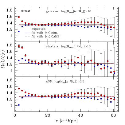
Figure 1: The ratio between the redshift-space and real-space two-point spherically averaged correlation functions, $\xi(s)/\xi(r)$, at $z=0.2$, for galaxies with $\log(M_{\rm STAR}[h^{-1}\,{\mbox{M}_{\odot}}])>10$ (top panel), clusters with $\log(M_{500}[h^{-1}\,{\mbox{M}_{\odot}}])>13$ (central panel), and AGN with $\log(M_{\rm BH}[h^{-1}\,{\mbox{M}_{\odot}}])>6.3$ (bottom panel). The redshift-space correlation functions have been measured directly from the simulation, while the real-space ones have been either measured from the simulation (red dots), or derived from the CAMB power spectrum (blue squares). The error bars represent the statistical noise as prescribed by Mo et al. (1992). The black solid lines show the expected values of $\xi(s)/\xi(r)$ at large scales predicted by Eq. (11b). The dotted blue and dashed red lines are the best-fit ratios estimated from the blue and red points, respectively.

5 Results

In this section, we present our main results obtained from mock samples of three different tracers – galaxies, clusters and AGN – using the two approaches described in §4. For each catalogue, we analyse six snapshots corresponding to the redshifts $z=\{0.2,0.52,0.72,1,1.5,2\}$. Moreover, at each redshift we consider different sample selections. In total, we analyse $270$ mock catalogues, whose main properties, including the number of objects in each sample, are reported in Tables LABEL:tab:table1, LABEL:tab:table2 and LABEL:tab:table3, and in Fig. 12 in Appendix A.

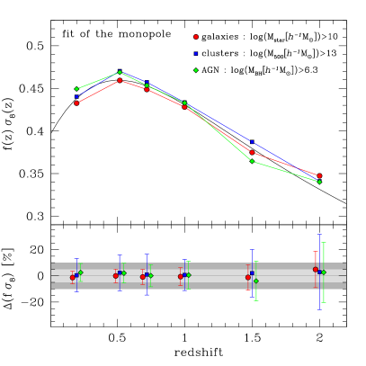
Figure 2: Top panel: the best-fit values of $f(z)\sigma_{8}(z)$ for galaxies with $\log(M_{\rm STAR}[h^{-1}\,{\mbox{M}_{\odot}}])>10$ (red dots), clusters with $\log(M_{500}[h^{-1}\,{\mbox{M}_{\odot}}])>13$ (blue squares), and AGN with $\log(M_{\rm BH}[h^{-1}\,{\mbox{M}_{\odot}}])>6.3$ (green diamonds), obtained with the method described in §5.1. The black line shows the function $\Omega_{\rm M}(z)^{0.545}\cdot\sigma_{8}(z)$, where $\Omega_{\rm M}(z)$ and $\sigma_{8}(z)$ are the known values of the simulation. Bottom panel: the percentage systematic errors on $f(z)\sigma_{8}(z)$, $[(f\sigma_{8})^{\rm measured}$-$(f\sigma_{8})^{\rm simulation}]/(f\sigma_{8})^{\rm simulation}\cdot 100$, that is the percentage differences between the points and the black line shown in the top panel. The error bars have been estimated with Eq. (19). The values reported have been slightly shifted for visual clarity. To guide the eyes, the light and grey shaded areas highlight the $5\%$ and $10\%$ error regions, respectively.

5.1 The linear growth rate from the clustering monopole

We start analysing the spherically averaged two-point correlation function – the clustering monopole – at large linear scales. The aim of this exercise is to investigate the accuracy of the RSD model in the simplest case possible, that is in the so-called Kaiser limit.

Fig. 1 shows the ratio between the redshift-space and real-space two-point correlation functions, $\xi(s)/\xi(r)$. Specifically, we show here the results obtained at $z=0.2$, for galaxies with $\log(M_{\rm STAR}[h^{-1}\,{\mbox{M}_{\odot}}])>10$, clusters with $\log(M_{500}[h^{-1}\,{\mbox{M}_{\odot}}])>13$, and AGN with $\log(M_{\rm BH}[h^{-1}\,{\mbox{M}_{\odot}}])>6.3$, as reported by the labels. These correspond to the upper left samples reported in Tables LABEL:tab:table1, LABEL:tab:table2 and LABEL:tab:table3. Results obtained from the other mock samples are similar, but more scattered due to the lower densities. The redshift-space correlation functions have been measured directly from the simulation, through the procedure described in §4. The real-space correlation functions have been estimated in two different ways. Either they are measured directly from the simulation, or they are derived from the linear CAMB power spectrum, and assuming a linear bias factor. The differences at small scales, $r\lesssim 5$ $h^{-1}\,\mbox{Mpc}$ , between the ratios computed with the measured (blue squares) and CAMB (red dots) real-space correlation functions are due to non-linear effects. We verified that using the non-linear CAMB power spectrum, via the HALOFIT routine (Smith et al. 2003), does not fully remove the discrepancy. Nevertheless, as we model here the large scale clustering, this has no effects on our results. On the other hand, the small discrepancies at scales $r\gtrsim 40$ $h^{-1}\,\mbox{Mpc}$ can introduce systematics, that however result smaller than the estimated uncertainties. The error bars in Fig. 1 show the statistical Poisson noise (Mo et al. 1992). Scales larger than $60$ $h^{-1}\,\mbox{Mpc}$ , not shown in the plot, are too noisy to affect the fit. More specifically, we verified that a convenient scale range to get robust results is $10<r[h^{-1}\,\mbox{Mpc}]<50$. The black solid lines show the expected values of $\xi(s)/\xi(r)$ at large scales, as predicted by Eq. (11b).

By modelling the clustering ratio, $\xi(s)/\xi(r)$, via Eq. (11a), it is possible to estimate the factor $\beta$. We do this by measuring both $\xi(s)$ and $\xi(r)$ from the simulation. The result is shown by the dotted blue lines in Fig. 1. Instead, to estimate $f\sigma_{8}$ from the monopole of the two-point correlation function, we use Eq. (11b). In this case the factor $b\sigma_{8}$ has to be fixed. This requires to estimate the real-space two-point correlation function of the DM. As described above, we obtain the latter by Fourier transforming the CAMB power spectrum. Moreover, to estimate the mean linear bias, a range of scales has to be chosen in Eq. (9). We compute the linear bias in the range $\bar{r}<r[$$h^{-1}\,\mbox{Mpc}$ $]<50$, where $\bar{r}$ is a free parameter that sets the minimum scale beyond which the bias is fairly scale-independent. Such a minimum scale depends on redshift and sample selection, and we estimate it for each sample considered. The dashed red lines are the best-fit ratios estimated with this method.

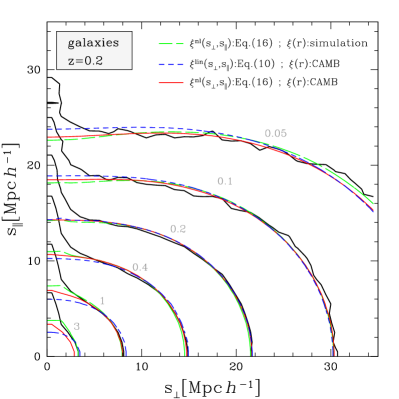
Figure 3: The iso-correlation contours of the redshift-space two-point correlation function, corresponding to the values $\xi(s_{\perp},s_{\parallel})$ $=[0.05,0.1,0.2,0.4,1,3]$, for galaxies with $\log(M_{\rm STAR}[h^{-1}\,{\mbox{M}_{\odot}}])>10$, at $z=0.2$ (black contours). The dot-dashed green and solid red contours show the best-fit model given by Eq. (16), with the real-space correlation function $\xi(r)$ measured from the simulation, and estimated from the CAMB power spectrum, respectively. The blue dashed contours show the linear best-fit model given by Eq. (10) with the CAMB real-space correlation function.

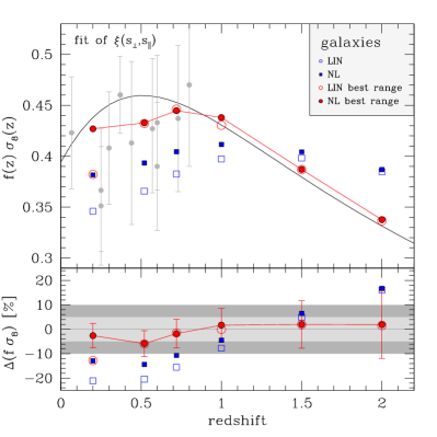
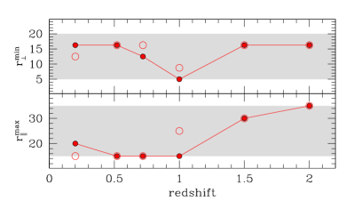
Figure 4: Top panel of the upper window: the best-fit values of $f(z)\sigma_{8}(z)$ for galaxies with $\log(M_{\rm STAR}[h^{-1}\,{\mbox{M}_{\odot}}])>10$. The open and solid blue squares show the values obtained by fitting the data with the models given by Eqs. (10) and (16), respectively, in the scale ranges $3<r_{\perp}[h^{-1}\,\mbox{Mpc}]<35$ and $3<r_{\parallel}[h^{-1}\,\mbox{Mpc}]<35$. The open and solid red dots have been obtained with the method described in §5.2.1, fitting the data with the models given by Eqs. (10) and (16), respectively. The black line shows the function $\Omega_{\rm M}(z)^{0.545}\cdot\sigma_{8}(z)$, where $\Omega_{\rm M}(z)$ and $\sigma_{8}(z)$ are the known values of the simulation. For comparison, the grey dots show a set of recent observational measurements from galaxy surveys (see §5.2.1). Bottom panel of the upper window: the percentage systematic errors on $f(z)\sigma_{8}(z)$, defined as $[(f\sigma_{8})^{\rm measured}$-$(f\sigma_{8})^{\rm simulation}]/(f\sigma_{8})^{\rm simulation}\cdot 100$, that is the percentage differences between the points and the black line shown in the top panel. To guide the eyes, the light and grey shaded areas highlight the $5\%$ and $10\%$ error regions. Lower window: best-fit values of $r_{\perp}^{\rm min}$ and $r_{\parallel}^{\rm max}$ of the method described in §5.2.1. The grey areas show the regions explored by the method.

As it can be seen by comparing red and blue lines, the two methods provide concordant results, both of them in agreement with the expectations. Indeed, the real-space correlation function provided by CAMB and assuming a linear bias is in reasonable agreement with the one measured directly from the simulation.

The constraints on $f\sigma_{8}$ as a function of redshift are shown in the upper panel of Fig. 2. As in Fig. 1, we show the results obtained for galaxies with $\log(M_{\rm STAR}[h^{-1}\,{\mbox{M}_{\odot}}])>10$, clusters with $\log(M_{500}[h^{-1}\,{\mbox{M}_{\odot}}])>13$, and AGN with $\log(M_{\rm BH}[h^{-1}\,{\mbox{M}_{\odot}}])>6.3$. The black line shows the function $\Omega_{\rm M}(z)^{0.545}\cdot\sigma_{8}(z)$, where $\Omega_{\rm M}(z)$ and $\sigma_{8}(z)$ are the values of the Magneticum simulation. In the lower panel we show the percentage systematic errors on $f\sigma_{8}$, defined as $[(f\sigma_{8})^{\rm measured}$-$(f\sigma_{8})^{\rm simulation}]/(f\sigma_{8})^{\rm simulation}\cdot 100$. The error bars have been estimated by propagating on $f\sigma_{8}$ the $\beta$ errors provided by the scaling formula presented in Bianchi et al. (2012), that gives the statistical errors as a function of bias, $b$, volume, $V$, and density, $n$:

$$\frac{\delta\beta}{\beta}\simeq Cb^{0.7}V^{-0.5}\exp\left(\frac{n_{0}}{b^{2}n}\right)\;,$$ (19)

where $n_{0}=1.7\cdot 10^{-4}\,h^{3}\,\mbox{Mpc}^{-3}$ and $C=4.9\cdot 10^{2}\,h^{-1.5}\,\mbox{Mpc}^{1.5}$. In this case, these error bars have to be considered just as lower limits, as the scaling formula has been calibrated based on fits of the full two-dimensional anisotropic correlation function $\xi(s_{\perp},s_{\parallel})$ . Moreover, they have been computed in different scale ranges and with Friends-of-Friends DM haloes, differently from this analysis, where we consider tracers hosted in DM sub-haloes. Using the full covariance matrix in this statistical analysis does not change our conclusions, as shown in Appendix C.

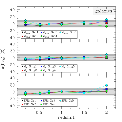
Figure 5: The percentage systematic errors on $f(z)\sigma_{8}(z)$ for galaxies, $[(f\sigma_{8})^{\rm measured}$-$(f\sigma_{8})^{\rm simulation}]/(f\sigma_{8})^{\rm simulation}\cdot 100$, as a function of redshift and sample selections, as indicated by the labels. $S1-S5$ refer to the five selection thresholds reported in Tables LABEL:tab:table1, LABEL:tab:table2 and LABEL:tab:table3, for the different tracers and properties used for the selection.

As demonstrated by Figs. 1 and 2, it is indeed possible to get almost unbiased constraints on $f\sigma_{8}$ from the monopole of the two-point correlation function, at all redshifts considered, and for both galaxies, clusters and AGN, provided that the linear bias is estimated at sufficiently large scales. The advantage of this method is the minimal number of free parameters necessary for the modelisation. However, the linear bias has to be assumed, or measured from other probes.

5.2 The linear growth rate from the anisotropic 2D clustering

To extract the full information from the redshift-space two-point correlation function, the anisotropic correlation $\xi(s_{\perp},s_{\parallel})$ or, alternatively, all the relevant multipoles have to be modelled. As discussed in §4, we consider the first approach. Differently from the analysis of §5.1, here we can jointly constrain the two terms $f\sigma_{8}$ and $b\sigma_{8}$. In this section we investigate the accuracy of the constraints on $f\sigma_{8}$ provided by the dispersion model, as a function of sample selection, with $b\sigma_{8}$ and $\sigma_{12}$ as free parameters.

5.2.1 Galaxies

We start presenting our results for the galaxy mock samples. The black lines of Fig. 3 show the iso-correlation contours of the redshift-space two-point correlation function, $\xi(s_{\perp},s_{\parallel})$ , for galaxies with $\log(M_{\rm STAR}[h^{-1}\,{\mbox{M}_{\odot}}])>10$, at $z=0.2$. The other lines are the best-fit models obtained with three different methods. The dot-dashed green lines are obtained by using the full non-linear dispersion model given by Eq. (16), with the real-space correlation function $\xi(r)$ measured directly from the simulation. The blue dashed and red solid contours are obtained with $\xi(r)$ estimated from the CAMB power spectrum, and by fitting the linear model given by Eq. (10) and the non-linear one by Eq. (16), respectively. The fitting is done in the scale ranges $3<r_{\perp}[h^{-1}\,\mbox{Mpc}]<35$ and $3<r_{\parallel}[h^{-1}\,\mbox{Mpc}]<35$.

As one can see, while all the three models provide a good description of the anisotropic clustering at scales larger than $\sim 5$ $h^{-1}\,\mbox{Mpc}$ , none of them can reproduce accurately the fingers-of-God pattern at small scales. This is expected for the blue contours, obtained without modelling the non-linear dynamics. For the other two cases, the discrepancy is due to the not sufficiently accurate description of non-linearities provided by the dispersion model. We verified that the minimum scales considered for the fit have a negligible impact on the fingers-of-God shape, that is we find the same results even considering scales smaller that 3 $h^{-1}\,\mbox{Mpc}$ in the fit. The green contours appear in better agreement with the measurements at small scales, due to the fact that the real-space correlation function is measured from the mock catalogue.

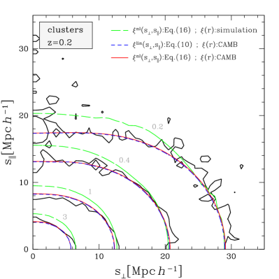
Figure 6: The iso-correlation contours of the redshift-space two-point correlation function, corresponding to the values $\xi(s_{\perp},s_{\parallel})$ $=[0.2,0.4,1,3]$, for clusters with $\log(M_{500}[h^{-1}\,{\mbox{M}_{\odot}}])>13$, at $z=0.2$ (black contours). The other contours are as in Fig. 3.

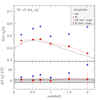
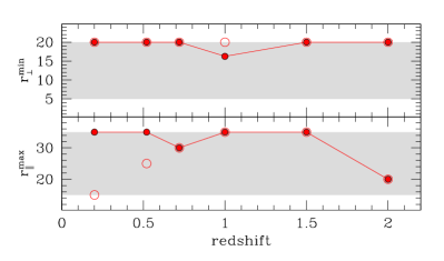
Figure 7: The best-fit values of $f(z)\sigma_{8}(z)$ for clusters with $\log(M_{500}[h^{-1}\,{\mbox{M}_{\odot}}])>13$. All the symbols are as in Fig. 4.

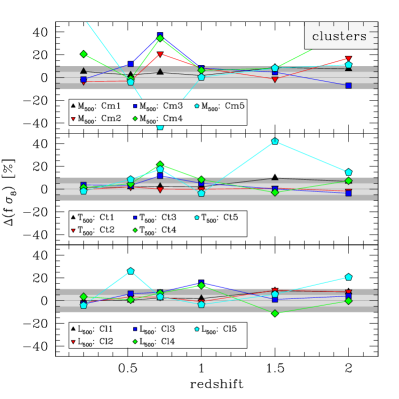
Figure 8: The percentage systematic errors on $f(z)\sigma_{8}(z)$ for clusters, as a function of redshift and sample selections. All symbols are as in Fig. 5.

The best-fit values of $f\sigma_{8}$ as a function of redshift are shown in the top panel of the upper window of Fig. 4. The open and solid blue squares show the values obtained by fitting the data with the models given by Eqs. (10) and (16), respectively, that is they correspond to the blue and red contours of Fig. 3 (at $z=0.2$). The bottom panel of the upper window shows the percentage systematic errors on $f\sigma_{8}$, that is $[(f\sigma_{8})^{\rm measured}$-$(f\sigma_{8})^{\rm simulation}]/(f\sigma_{8})^{\rm simulation}\cdot 100$.

As it can be seen, the best-fit values of $f\sigma_{8}$ result strongly biased with respect to the true ones, with a systematic error that depends on the redshift. At $z=0.2$, we get an underestimation of $\sim 10$ ($20$) $\%$ with the non-linear (linear) dispersion model, at $z=1$ the error reduces to $\sim 5$ ($8$)$\%$, while at $z=2$ we get an overestimation of $\sim 20\%$, with both linear and non-linear modelling. This result is fairly in agreement with what found by Bianchi et al. (2012) at $z=1$, although the two analyses are not directly comparable, as Bianchi et al. (2012) considered a sample of Friends-of-Friends DM haloes, slightly affected by fingers-of-God. As expected, the convolution given by Eq. (16) reduces the systematic error on $f\sigma_{8}$, especially at low redshifts. However, it does not totally remove the discrepancies, in agreement with previous findings (e.g. Mohammad et al. 2016, and references therein). For comparison, the grey dots of Fig. 4 show a set of recent observational measurements of $f\sigma_{8}$ from large galaxy surveys: 6dFGS at $z=0.067$ (Beutler et al. 2012); SDSS(DR7) Luminous Red Galaxies at $z=0.25,0.37$ (Samushia et al. 2012) from scales lower than $60$ and $200$ $h^{-1}\,\mbox{Mpc}$ ; BOSS at $z=0.3,0.57,0.6$ (Tojeiro et al. 2012; Reid et al. 2012); WiggleZ at $z=0.44,0.6,0.73$ (Blake et al. 2012); VIPERS at $z=0.8$ (de la Torre et al. 2013). These results have been obtained using different RSD models, most of them more accurate than the dispersion model considered in this work. Nevertheless, many of these measurements underestimate $f\sigma_{8}$ with respect to GR+$\Lambda$CDM predictions (see e.g. Macaulay et al. 2013). In line with our findings, this could be explained, at least partially, by model uncertainties still present in the more sophisticated RSD models considered.

The direct way to reduce these systematics is to improve the modelisation of RSD at non-linear scales (see e.g. Scoccimarro 2004; Taruya et al. 2010; Seljak & McDonald 2011; Wang et al. 2014; de la Torre et al. 2013). We explore here a different approach, investigating the dependency of the systematic error on the comoving scales considered in the analysis. In the forthcoming plots, we show the results obtained by repeating our fitting procedure for different values of the minimum perpendicular separation and the maximum parallel separation used in the fit, that is $r_{\perp}^{\rm min}$ and $r_{\parallel}^{\rm max}$. By increasing the value of $r_{\perp}^{\rm min}$ we can cut the region more affected by fingers-of-God anisotropies, while by reducing $r_{\parallel}^{\rm max}$ we avoid the region more affected by shot noise. As we verified, changing also $r_{\perp}^{\rm max}$ and $r_{\parallel}^{\rm min}$, or adopting different scale selection criteria, do not affect significantly the results. The aim here is to search for optimal regions in this plane to possibly get unbiased constraints. As non-linear dynamics impact on different scales for different redshifts and biases of the tracers, we expect that the best values of $r_{\perp}^{\rm min}$ and $r_{\parallel}^{\rm max}$, that is the ones that minimise systematics, will be different for different sample selections.

The results of this analysis are shown in Fig. 4 with open and solid red dots, obtained by fitting the data with the model given by Eqs. (10) and (16), respectively, that is by considering either the linear or the non-linear RSD model. We explore the ranges $5<r_{\perp}^{\rm min}[h^{-1}\,\mbox{Mpc}]<20$ and $15<r_{\parallel}^{\rm max}[h^{-1}\,\mbox{Mpc}]<35$, highlighted by the grey areas in the bottom panels of the lower window of Fig. 4. Specifically, we consider a 10x10 grid in the $r_{\perp}^{\rm min}$, $r_{\parallel}^{\rm max}$ plane. The best-fit values of $r_{\perp}^{\rm min}$ and $r_{\parallel}^{\rm max}$, shown in the bottom panels of the lower window, are the ones that minimise the systematic error on $f\sigma_{8}$. The ranges considered are large enough to get systematic errors on $f\sigma_{8}$ lower than $\sim 5\%$. Indeed, for proper values of $r_{\perp}^{\rm min}$ and $r_{\parallel}^{\rm max}$, it is possible to significantly reduce the systematic error on $f\sigma_{8}$ at all redshifts, without having to improve the treatment of non-linearities. The error bars have been estimated using the scaling formula given by Eq. 19.

Both the linear and non-linear dispersion models provide similar results when $r_{\perp}^{\rm min}$ and $r_{\parallel}^{\rm max}$ are kept free. In other words, it seems more convenient simply to not consider the scales where non-linear effects have a non-negligible impact, rather than to try modelling them with the empirical description provided by Eq. (16).

These results show that i) it is possible to reduce significantly the systematics in RSD constraints, even with the dispersion model, by cutting the $r_{\perp}^{\rm min}$, $r_{\parallel}^{\rm max}$ plane conveniently, and ii) the optimal $r_{\perp}^{\rm min}$, $r_{\parallel}^{\rm max}$ range depends on sample selection, thus it cannot be just fixed in multi-tracer analyses. As it can be seen in Fig. 4, we do not find any clear trend of $r_{\perp}^{\rm min}$ and $r_{\parallel}^{\rm max}$ as a function of redshift, as it would be expected if the systematics were caused by non-linearities. This is possibly caused by the not sufficiently large volumes considered. The analysis of larger data sets, that we defer to a future work, will hopefully clarify this point.

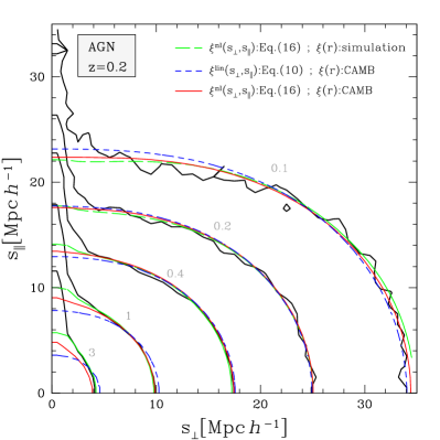
Figure 9: The iso-correlation contours of the redshift-space two-point correlation function, corresponding to the values $\xi(s_{\perp},s_{\parallel})$ $=[0.1,0.2,0.4,1,3]$, for AGN with $\log(M_{\rm BH}[h^{-1}\,{\mbox{M}_{\odot}}])>6.3$, at $z=0.2$ (black contours). The other contours show the best-fit models, as in Fig. 3.

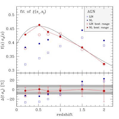
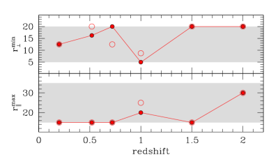
Figure 10: The best-fit values of $f(z)\sigma_{8}(z)$ for AGN with $\log(M_{\rm BH}[h^{-1}\,{\mbox{M}_{\odot}}])>6.3$. All the symbols are as in Fig. 4.

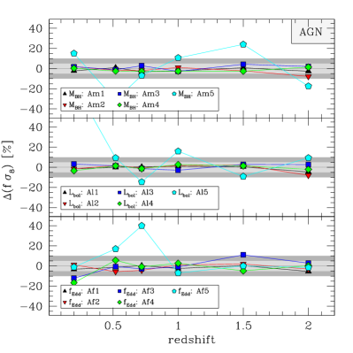
Figure 11: The percentage systematic errors on $f(z)\sigma_{8}(z)$ for AGN, as a function of redshift and sample selections. All symbols are as in Fig. 5.

For completeness, we then apply our method to several subsamples with different selections. Specifically, we consider galaxy catalogues selected in stellar mass, $M_{\rm STAR}$, g-band absolute magnitude, $M_{g}$, and star formation rate, SFR. The selection thresholds considered and the number of galaxies in each sample are reported in Table LABEL:tab:table1. The percentage systematic errors on $f\sigma_{8}$ are reported in Fig. 5, as a function of redshift and sample selections, as indicated by the labels. The result is quite remarkable: it is indeed possible to get almost unbiased constraints on $f\sigma_{8}$ with the dispersion model, independent of sample selections, provided that $r_{\perp}^{\rm min}$ and $r_{\parallel}^{\rm max}$ are chosen conveniently. For the largest galaxy sample shown in Fig. 2, the preferred value of $r_{\perp}^{\rm min}$ is $\sim 15$ $h^{-1}\,\mbox{Mpc}$ at low and high redshifts, and $\sim 5$ $h^{-1}\,\mbox{Mpc}$ around $z=1$, while $r_{\parallel}^{\rm max}$ is $\sim 15$ $h^{-1}\,\mbox{Mpc}$ at low redshifts, and increases up to $\sim 35$ $h^{-1}\,\mbox{Mpc}$ at $z=2$. Again, we do not find any clear trend of $r_{\perp}^{\rm min}$ and $r_{\parallel}^{\rm max}$ as a function of redshift or sample bias.

Overall, all of these results show that our modelling of RSD is mostly sensitive to the lower fitting cut-off, depending on how the tracers relate to the underlying mass. Indeed, the effect of the different selections considered here is just to select subsamples of haloes of different masses (hence bias) hosting the observed galaxies. As noted above, this has to be considered in multi-tracer analyses, where a single sample selection might introduce systematics.

5.2.2 Galaxy groups and clusters

In this section, we perform the same analysis presented in §5.2.1 on the mock samples of galaxy groups and clusters. To simplify the discussion, in the following we will use the term clusters to refer to all of these objects, though the less massive ones should be considered as galaxy groups, or just haloes, from an observational perspective (see Table LABEL:tab:table2).

Fig. 6 shows the iso-correlation contours of the redshift-space two-point correlation function of clusters with $\log(M_{500}[h^{-1}\,{\mbox{M}_{\odot}}])>13$, at $z=0.2$. The other contours are the best-fit models, as in Fig. 3. As it can be seen, the fingers-of-God anisotropies are almost absent, differently from the galaxy correlation function shown in Fig. 3, due to the lower values of non-linear motions of clusters at small scales. This makes the convolution of Eq. (16) negligible, as it can be seen comparing the dashed blue and solid red lines. Interestingly, when the real-space correlation function $\xi(r)$ is measured from the mocks (green contours), the dispersion model fails to match the small-scale clustering shape. This is primarily caused by the paucity of the cluster sample. Due to the low number of cluster pairs at small separations, the small-scale clustering cannot be estimated accurately, thus introducing systematics in the model. On the contrary, when $\xi(r)$ is estimated from CAMB, the small-scale clustering shape can be accurately described. For visual clarity, we have shown here only the iso-correlation contours down to $\xi(s_{\perp},s_{\parallel})$ $=0.2$, as for lower values they appear too scattered.

Fig. 7 shows the best-fit values of $f\sigma_{8}$ as a function of redshift. In contrast with what we found with galaxies, the constraints on the linear growth rate obtained in the scale ranges $3<r_{\perp}[h^{-1}\,\mbox{Mpc}]<35$ and $3<r_{\parallel}[h^{-1}\,\mbox{Mpc}]<35$ (blue squares) result severely overestimated at all redshifts, independent of using the linear or the non-linear dispersion model. To investigate how these systematics depend on the scale range considered in the fit, we repeat the same analysis described in §5.2.1, keeping free the parameters $r_{\perp}^{\rm min}$ and $r_{\parallel}^{\rm max}$. The result is shown by the red dots in Fig. 7. As one can see, we are able to substantially reduce the systematics on $f\sigma_{8}$, at all redshifts. This is obtained by cutting the small perpendicular separations, limiting the analysis at $r_{\perp}\gtrsim 20$ $h^{-1}\,\mbox{Mpc}$ , as shown in the lower window of Fig. 7.

These results appear in overall agreement with what previously found by Bianchi et al. (2012), where systematic errors become positive for DM halo masses larger than $10^{13}h^{-1}\,{\mbox{M}_{\odot}}$, that is for group masses and above. This represents a nice confirmation, not related to the specific simulation or halo/cluster selection, but only to the dynamics of haloes of large masses.

Then, we consider several cluster subsamples selected in mass, $M_{500}$, temperature, $T_{500}$, and luminosity, $L_{500}$, whose main properties are reported in Table LABEL:tab:table2. Fig. 8 shows the percentage systematic errors on $f\sigma_{8}$ as a function of redshift and sample selections. For the largest samples analysed we do not get any significant bias on $f\sigma_{8}$, similarly to what we found with galaxies. However, when selecting too few objects, the results appear quite scattered, though without systematic trends. Indeed, the advantages resulting from the low fingers-of-God anisotropies compensate with the paucity of cluster pairs at small scales. Summarising, it seems possible to get unbiased constraints on the linear growth rate from the RSD of galaxy clusters, but the cluster sample has to be sufficiently numerous.

5.2.3 AGN

Finally, we analyse the AGN mock samples. The results are shown in Figs. 9, 10 and 11, that are the analogous of the plots presented in the previous two sections for galaxies and clusters. As expected, we find similar results to the ones found with galaxies. Differently from the cluster case, the fingers-of-God are clearly evident in the AGN correlation function, and not accurately described by the dispersion model, as it can be seen in Fig. 9. Nevertheless, the convolution of Eq. (16) significantly helps in reducing the systematic error on $f\sigma_{8}$, even more than what we found when analysing the galaxy sample, as evident by comparing Figs. 3 and 9. Also in this case, it is possible to get almost unbiased constraints on $f\sigma_{8}$ at all redshifts and for the different selections considered, provided that the analysis is restricted at $r_{\perp}^{\rm min}\gtrsim 15$ $h^{-1}\,\mbox{Mpc}$ and $r_{\parallel}^{\rm max}\lesssim 15$ $h^{-1}\,\mbox{Mpc}$ . Specifically, we considered here AGN catalogues selected in BH mass, $M_{\rm BH}$, bolometric luminosity, $L_{\rm bol}$, and Eddington factor, $f_{\rm Edd}$, as reported in Table LABEL:tab:table3. Only the AGN samples with the lower number of objects analysed here (cyan points in Fig. 11) are not large enough to provide robust constraints on $f\sigma_{8}$.

6 Discussion

The results presented in this paper extend the previous work by Bianchi et al. (2012), who analysed mock samples of DM haloes at $z=1$. One of the main differences with respect to that work is that here we used galaxy, cluster and AGN simulated catalogues, that are more directly comparable to observational samples. Moreover, we investigated the systematic errors of $f\sigma_{8}$, instead of $\beta$, and extended the analysis at different redshifts and sample selections. The use of these simulated objects as test particles provides a better treatment of non-linearities in small-scale dynamics, that translates to a more realistic description of the fingers-of-God in the redshift-space galaxy and AGN clustering, as it can be seen in Figs. 3 and 9. On the other hand, the selected cluster samples are more similar to the DM halo samples analysed by Bianchi et al. (2012), as expected, with fingers-of-God anisotropies almost absent, as shown in Fig. 6. Nevertheless, the Magneticum samples provide cluster properties that allowed us to apply more realistic selections.

One of the main results found by Bianchi et al. (2012) is that, when using the dispersion model, the systematic errors on the linear growth rate are positive for DM haloes with masses lower than $\sim 10^{13}h^{-1}\,{\mbox{M}_{\odot}}$, and negative otherwise (see also Okumura & Jing 2011; Marulli et al. 2012b). Our findings reinforce these conclusions. Indeed, regardless of the specific selections considered, the overall trends of our systematic errors depend ultimately on the mass of the DM haloes hosting the selected tracers.

Moreover, extending the Bianchi et al. (2012) analysis, we investigated how the systematic errors depend on the comoving scales considered. Our main finding is that it is possible to substantially reduce the systematic errors at all redshifts and selections by restricting the analysis in a proper subregion of the $r_{\perp}-r_{\parallel}$ plane. The latter depends on the properties of the selected objects, specifically on the mass of the host halo, due to the difficulties in modelling the non-Gaussian nature of the velocity probability density function of the tracers.

7 Conclusions

Clustering anisotropies in redshift-space are one of the most effective probes to test Einstein’s General Relativity on large scales. Though only galaxy samples have been considered so far for these analyses, other astronomical tracers, such as clusters and AGN, will be used in the next future, aimed at maximising the dynamic and redshift ranges where to constrain the linear growth rate of cosmic structures. In particular, clusters of galaxies can be efficiently used to probe the low redshift Universe. Their large bias and low velocity dispersion at small scales make them optimal tracers for large scale structure analyses (Sereno et al. 2015; Veropalumbo et al. 2014, 2016). On the other hand, AGN samples can be exploited to push the GR test on larger redshifts.

In this work, we made use of both galaxy, cluster and AGN mock samples extracted from the Magneticum, a cosmological hydrodinamic simulation of the standard $\Lambda$CDM Universe, to investigate the accuracy of the widely used dispersion model as a function of scale and sample selection. Instead of analysing the clustering multipoles, we preferred to extract $f\sigma_{8}$ constraints from the monopole only, or from the full 2D anisotropic correlation $\xi(s_{\perp},s_{\parallel})$ . This allowed us to explore the $r_{\perp}-r_{\parallel}$ plane, aimed at finding the optimal range of scales to minimise systematic uncertainties.

The main results of this analysis are the following.

• It is possible to get almost unbiased constraints on $f\sigma_{8}$ by modelling the large-scale monopole of the two-point correlation function with the Kaiser limit of the dispersion model (Eq. 11b), provided that the linear bias factor $b\sigma_{8}$ is known. The latter has to be estimated at sufficiently large scales, to avoid non-linearities. With real data, the linear bias can be estimated either with the deprojection technique, or from the three-point correlation function, or by combining clustering and lensing measurements (see the discussion in §4).

• When higher multipoles are considered, $f\sigma_{8}$ and $b\sigma_{8}$ can be jointly constrained, and the statistical error on $f\sigma_{8}$ is substantially reduced (see e.g. de la Torre et al. 2013; Petracca et al. 2016). However, systematic errors can arise if non-linearities are not treated accurately, such as with the dispersion model (Eqs. 10-17). On the other hand, the analysis shown in this paper demonstrates that it is still possible to reduce the systematic errors on $f\sigma_{8}$ if the range of scales used to model RSD is chosen appropriately. The latter depends on the properties of the tracers. We do not find however any clear prescription to relate these scale ranges to the sample properties.

• If the linear growth rate is estimated from the RSD of either galaxies or AGN, the value of $f\sigma_{8}$ will be underestimated at $z\lesssim 1$, and overestimated at larger redshifts, when the fit is performed in the fixed range of scales $3<r_{\perp},r_{\parallel}[h^{-1}\,\mbox{Mpc}]<35$. With $r_{\perp}^{\rm min}\sim 15$ $h^{-1}\,\mbox{Mpc}$ and $r_{\parallel}^{\rm max}\sim 20$ $h^{-1}\,\mbox{Mpc}$ , we get almost unbiased constraints. However, the proper values of $r_{\perp}^{\rm min}$ and $r_{\parallel}^{\rm max}$ depend on sample selection, and should be fixed differently for each sample analysed, calibrating the analysis using specific mock catalogues.

• If the RSD of galaxy groups and clusters are modelled in the range of scales $3<r_{\perp},r_{\parallel}[h^{-1}\,\mbox{Mpc}]<35$, the value of $f\sigma_{8}$ results severely overestimated at all redshifts. The results at $z=1$ appear in overall agreement with what found by Bianchi et al. (2012). The systematic error can be reduced if the fit is performed at larger scales, as expected due to the low number of cluster pairs at small separations. Specifically, with $r_{\perp}^{\rm min}\sim 20$ $h^{-1}\,\mbox{Mpc}$ , we get unbiased constraints, but only for the densest group samples. The paucity of the most massive cluster samples does not allow us to obtain robust results.

To summarise, as the dispersion model cannot accurately describe the non-linear motions at small scales, the constraints on $f\sigma_{8}$ can be biased. At the present time, it is difficult to include model uncertainties in this kind of analyses, and even more to improve the RSD modelling at small scales (see e.g. de la Torre & Guzzo 2012; Bianchi et al. 2015, and references therein). Instead of trying to improve the model, in this analysis we investigated how the systematic errors on the linear growth rate caused by model uncertainties depend on the comoving scales considered. As we have shown, in order to reduce these systematics it is necessary to restrict the analysis in a proper subregion of the $r_{\perp}-r_{\parallel}$ plane. More specifically, we found that it is enough to choose a proper value for $r_{\perp}^{\rm min}$ and $r_{\parallel}^{\rm max}$. Indeed, as we verified, changing also $r_{\perp}^{\rm max}$ and $r_{\parallel}^{\rm min}$ does not affect significantly the results.

Overall, we find that, in order to reduce the systematics in the $f\sigma_{8}$ measurements, it is more convenient simply to not consider the small scales where non-linear effects distort significantly the clustering shape, rather than to try modelling them with the empirical description provided by the dispersion model given by Eq. (16). The drawback of this approach is to inevitably increase the statistic error on $f\sigma_{8}$. Moreover, the $r_{\perp}-r_{\parallel}$ region to be selected depends on the properties of the tracers, and should be determined using suitable mock catalogues. On the other hand, without a sufficiently accurate modelisation of non-linear dynamics at small scales, this approach is the only one possible to get unbiased constraints.

This can have a non-negligible impact on multiple tracer analyses (see e.g. McDonald & Seljak 2009; Blake et al. 2013; Marín et al. 2016, and references therein) if the RSD are modelled at small non-linear scales with the dispersion model. To avoid different systematic errors on the linear growth rate estimated from the small-scale RSD of different tracers, the $r_{\perp}-r_{\parallel}$ plane analysed should be different for each sample. On the other hand, in multiple tracer techniques that require to analyse different samples at the same scales, it is necessary to limit the analysis at large enough scales where systematic errors are lower than statistical errors for all the different tracers. And the same when joining together different redshifts, where RSD constraints can be differently biased.

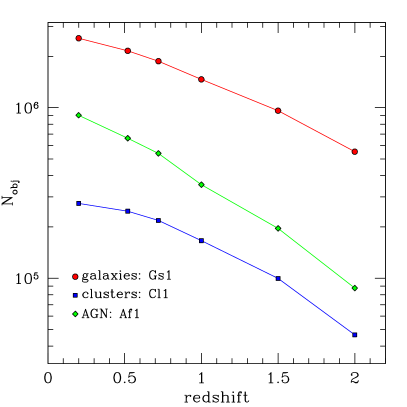
Figure 12: The number of mock galaxies (red dots), clusters (blue squares) and AGN (green diamonds) as a function of redshift, for the three selections: Gs1, Cl1, Af1 (see Tables LABEL:tab:table1, LABEL:tab:table2 and LABEL:tab:table3).

Appendix A The main properties of the selected samples

Tables LABEL:tab:table1, LABEL:tab:table2 and LABEL:tab:table3 report the main properties of the mock samples analysed in this work. We consider only integral catalogues. The quantities min and max reported in the Tables are the minimum and maximum thresholds used for the selections, while median is the median of the sample distributions. As it can be seen, we adopt suitable sample selections to have a minimum of $\sim 50000$ objects in the smallest galaxy samples, and $\sim 10000$ objects in the smallest cluster and AGN samples. As an illustrative example, Fig. 12 shows the number of mock galaxies, clusters and AGN as a function of redshift, for three different selections, as indicated by the labels.

Appendix B The effect of random catalogue number densities

We test the impact of our assumptions in constructing the random catalogues by repeating the full statistical analysis on a subset of the mock samples, using random catalogues with different number densities. Fig. 13 shows an example case obtained from the sample of mock galaxies at $z=0.2$. The lines show the ratio $\Delta\xi/\sigma_{\xi}$ as a function of scales, where $\Delta\xi=\xi_{N_{R}=3}-\xi_{N^{\prime}_{R}}$, with $N_{R}$ being the ratio between the number of random objects and galaxies, and $\sigma_{\xi}$ is the estimated statistical uncertainty. The different lines refer to the values $N^{\prime}_{R}=1,5,10$. The effect of different random number densities on the measured correlation functions is marginal, considering the estimated uncertainties. As verified, the net effect on the final RSD constraints is also negligible.

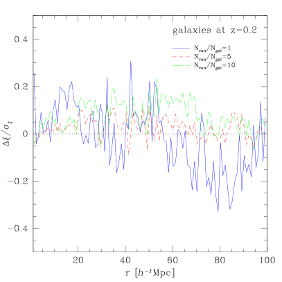
Figure 13: The ratio $\Delta\xi/\sigma_{\xi}$ as a function of scales obtained from the sample of mock galaxies at $z=0.2$, where $\Delta\xi=\xi_{N_{R}=3}-\xi_{N^{\prime}_{R}}$, with $N_{R}$ being the ratio between the number of random objects and galaxies, and $\sigma_{\xi}$ is the estimated statistical uncertainty. Blue, red and green lines refer to the values of $N^{\prime}_{R}=1,5,10$, respectively.

Appendix C The effect of covariance matrix approximations

All the results presented in this paper have been obtained by assuming Poisson errors in clustering measurements and by neglecting the off-diagonal elements of the covariance matrix. Both of these approximations can introduce systematics in the inferred cosmological constraints. However, as we verified, they do not impact significantly our present conclusions, introducing just marginal differences in the final obtained constraints, considering the estimated uncertainties. Fig. 14 shows the difference in the $f\sigma_{8}$ measurements obtained with diagonal Poisson errors and by considering the full covariance matrix assessed with either jackknife or bootstrap techniques, divided by the $1\sigma$ uncertainty on $f\sigma_{8}$. We use $125$ jackknife/bootstrap mock realisations to compute the covariance matrices (see Veropalumbo et al. 2016, for more details on the used methods and codes). As it can be seen, the effect of assuming negligible off-diagonal elements in the covariance matrix is not statistically significant. Moreover, the off-diagonal elements in the covariance matrix can introduce systematics and spurious scatter in the inferred cosmological constraints, if not properly estimated with a sufficiently large number of mocks. The above considerations motivated our choice of neglecting off-diagonal terms in the analyses presented in this paper, in line with previous similar works (see e.g. Bianchi et al. 2015; Petracca et al. 2016).

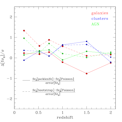
Figure 14: The difference between $f\sigma_{8}$ measurements obtained with diagonal Poisson errors and by considering the full covariance matrix assessed with either the jackknife (solid lines) or the bootstrap (dashed lines) techniques, divided by the $1\sigma$ uncertainty on $f\sigma_{8}$, as a function of redshift. Red, blue and green symbols refer to galaxy, cluster and AGN samples, respectively.

Table 1: Main properties of the samples of galaxies analysed in the paper.

redshift	$\log(M_{\rm STAR}[h^{-1}\,{\mbox{M}_{\odot}}])$						$M_{g}$						$\log(SFR[{\mbox{M}_{\odot}/year}])$
	sample	min	max	median	objects		sample	min	max	median	objects		sample	min	max	median	objects
${\bf 0.2}$	Gm1	$10.00$	$13.24$	$10.78$	$2565412$		Gmg1	$-20.00$	$-27.39$	$-21.90$	$2555977$		Gs1	$1.00$	$3.40$	$1.38$	$1460374$
	Gm2	$10.45$		$10.98$	$1881270$		Gmg2	$-20.94$		$-21.93$	$2465212$		Gs2	$1.24$		$1.47$	$1057208$
	Gm3	$10.90$		$11.13$	$1080529$		Gmg3	$-21.87$		$-22.31$	$1333968$		Gs3	$1.48$		$1.64$	$509094$
	Gm4	$11.35$		$11.55$	$255117$		Gmg4	$-22.81$		$-23.19$	$267639$		Gs4	$1.72$		$1.86$	$169018$
	Gm5	$11.79$		$11.96$	$50000$		Gmg5	$-23.74$		$-24.12$	$49995$		Gs5	$1.96$		$2.08$	$49996$
${\bf 0.52}$	Gm1	$10.00$	$13.10$	$10.73$	$2167365$		Gmg1	$-20.00$	$-27.08$	$-21.65$	$2154603$		Gs1	$1.00$	$3.33$	$1.45$	$1432387$
	Gm2	$10.42$		$10.93$	$1556875$		Gmg2	$-20.88$		$-21.70$	$1985640$		Gs2	$1.27$		$1.54$	$1087917$
	Gm3	$10.84$		$11.11$	$905634$		Gmg3	$-21.76$		$-22.21$	$913480$		Gs3	$1.54$		$1.71$	$550535$
	Gm4	$11.27$		$11.46$	$245678$		Gmg4	$-22.64$		$-23.07$	$231625$		Gs4	$1.80$		$1.95$	$181393$
	Gm5	$11.69$		$11.84$	$50000$		Gmg5	$-23.52$		$-23.88$	$49993$		Gs5	$2.07$		$2.20$	$49998$
${\bf 0.72}$	Gm1	$10.00$	$13.03$	$10.69$	$1894509$		Gmg1	$-20.00$	$-26.78$	$-21.53$	$1872485$		Gs1	$1.00$	$3.35$	$1.50$	$1360951$
	Gm2	$10.40$		$10.90$	$1347360$		Gmg2	$-20.86$		$-21.62$	$1657323$		Gs2	$1.28$		$1.58$	$1069332$
	Gm3	$10.81$		$11.10$	$788388$		Gmg3	$-21.72$		$-22.19$	$708654$		Gs3	$1.56$		$1.75$	$569550$
	Gm4	$11.21$		$11.39$	$242502$		Gmg4	$-22.58$		$-23.05$	$209604$		Gs4	$1.84$		$2.00$	$190113$
	Gm5	$11.61$		$11.77$	$50000$		Gmg5	$-23.44$		$-23.79$	$49984$		Gs5	$2.13$		$2.25$	$49999$
${\bf 1}$	Gm1	$10.00$	$12.92$	$10.62$	$1507943$		Gmg1	$-20.00$	$-26.78$	$-21.43$	$1465209$		Gs1	$1.00$	$3.41$	$1.58$	$1206017$
	Gm2	$10.37$		$10.84$	$1055108$		Gmg2	$-20.84$		$-21.55$	$1229380$		Gs2	$1.30$		$1.65$	$994050$
	Gm3	$10.75$		$11.07$	$620010$		Gmg3	$-21.69$		$-22.15$	$490496$		Gs3	$1.60$		$1.81$	$572970$
	Gm4	$11.12$		$11.28$	$247210$		Gmg4	$-22.53$		$-23.09$	$171265$		Gs4	$1.89$		$2.05$	$199961$
	Gm5	$11.49$		$11.65$	$49999$		Gmg5	$-23.38$		$-23.71$	$49689$		Gs5	$2.19$		$2.32$	$50000$
${\bf 1.5}$	Gm1	$10.00$	$12.79$	$10.55$	$1028296$		Gmg1	$-20.00$	$-26.09$	$-21.28$	$959724$		Gs1	$1.00$	$3.53$	$1.67$	$921472$
	Gm2	$10.33$		$10.76$	$711625$		Gmg2	$-20.79$		$-21.44$	$760311$		Gs2	$1.31$		$1.72$	$811432$
	Gm3	$10.67$		$10.99$	$421555$		Gmg3	$-21.58$		$-21.96$	$298389$		Gs3	$1.62$		$1.87$	$516807$
	Gm4	$11.00$		$11.19$	$204649$		Gmg4	$-22.38$		$-23.28$	$86610$		Gs4	$1.93$		$2.09$	$206667$
	Gm5	$11.33$		$11.48$	$50000$		Gmg5	$-23.17$		$-23.56$	$49994$		Gs5	$2.24$		$2.37$	$50000$
${\bf 2}$	Gm1	$10.00$	$12.49$	$10.48$	$618406$		Gmg1	$-20.00$	$-25.87$	$-21.17$	$552844$		Gs1	$1.00$	$3.54$	$1.74$	$589434$
	Gm2	$10.29$		$10.67$	$425026$		Gmg2	$-20.51$		$-21.27$	$477671$		Gs2	$1.31$		$1.78$	$543876$
	Gm3	$10.58$		$10.88$	$254679$		Gmg3	$-21.02$		$-21.48$	$330108$		Gs3	$1.61$		$1.90$	$386208$
	Gm4	$10.87$		$11.10$	$130253$		Gmg4	$-21.53$		$-21.85$	$148563$		Gs4	$1.92$		$2.11$	$179827$
	Gm5	$11.16$		$11.30$	$49999$		Gmg5	$-22.05$		$-22.49$	$47889$		Gs5	$2.23$		$2.36$	$49996$

Table 2: Main properties of the samples of galaxy groups and clusters analysed in the paper.

redshift	$\log(M_{500}[h^{-1}\,{\mbox{M}_{\odot}}])$						$T_{500}[keV]$						$\log(L_{500}[erg/s])$
	sample	min	max	median	objects		sample	min	max	median	objects		sample	min	max	median	objects
${\bf 0.2}$	Cm1	$13.00$	$14.97$	$13.26$	$103201$		Ct1	$0.10$	$8.27$	$0.29$	$274787$		Cl1	$42.00$	$46.57$	$42.51$	$249655$
	Cm2	$13.18$		$13.41$	$63705$		Ct2	$0.19$		$0.35$	$215729$		Cl2	$42.41$		$42.75$	$153119$
	Cm3	$13.37$		$13.58$	$36858$		Ct3	$0.34$		$0.54$	$110534$		Cl3	$42.83$		$43.16$	$65040$
	Cm4	$13.55$		$13.74$	$19963$		Ct4	$0.64$		$0.89$	$39922$		Cl4	$43.24$		$43.54$	$26922$
	Cm5	$13.74$		$13.90$	$9999$		Ct5	$1.18$		$1.52$	$9902$		Cl5	$43.66$		$43.92$	$9977$
${\bf 0.52}$	Cm1	$13.00$	$14.97$	$13.23$	$84523$		Ct1	$0.10$	$7.94$	$0.30$	$247341$		Cl1	$42.00$	$46.09$	$42.64$	$239836$
	Cm2	$13.16$		$13.37$	$53798$		Ct2	$0.18$		$0.36$	$198050$		Cl2	$42.43$		$42.78$	$180659$
	Cm3	$13.31$		$13.50$	$32449$		Ct3	$0.33$		$0.52$	$109150$		Cl3	$42.87$		$43.19$	$75378$
	Cm4	$13.47$		$13.64$	$18518$		Ct4	$0.61$		$0.84$	$40267$		Cl4	$43.30$		$43.59$	$29210$
	Cm5	$13.62$		$13.79$	$10000$		Ct5	$1.11$		$1.42$	$9959$		Cl5	$43.73$		$43.98$	$9991$
${\bf 0.72}$	Cm1	$13.00$	$14.69$	$13.22$	$69404$		Ct1	$0.10$	$6.57$	$0.31$	$218241$		Cl1	$42.00$	$46.24$	$42.77$	$215861$
	Cm2	$13.13$		$13.33$	$45804$		Ct2	$0.18$		$0.36$	$176278$		Cl2	$42.44$		$42.83$	$187288$
	Cm3	$13.27$		$13.45$	$29018$		Ct3	$0.32$		$0.50$	$103154$		Cl3	$42.89$		$43.20$	$84083$
	Cm4	$13.40$		$13.57$	$17408$		Ct4	$0.58$		$0.80$	$39329$		Cl4	$43.33$		$43.61$	$31049$
	Cm5	$13.54$		$13.69$	$9999$		Ct5	$1.04$		$1.31$	$9973$		Cl5	$43.77$		$44.02$	$9992$
${\bf 1}$	Cm1	$12.50$	$14.58$	$12.81$	$167773$		Ct1	$0.10$	$5.85$	$0.31$	$166270$		Cl1	$42.00$	$46.15$	$42.88$	$166445$
	Cm2	$12.72$		$12.97$	$104160$		Ct2	$0.17$		$0.36$	$137909$		Cl2	$42.44$		$42.91$	$156759$
	Cm3	$12.95$		$13.15$	$55569$		Ct3	$0.30$		$0.47$	$86893$		Cl3	$42.88$		$43.20$	$84056$
	Cm4	$13.17$		$13.34$	$25461$		Ct4	$0.52$		$0.72$	$36186$		Cl4	$43.32$		$43.59$	$32064$
	Cm5	$13.39$		$13.54$	$10000$		Ct5	$0.91$		$1.15$	$9991$		Cl5	$43.76$		$43.99$	$9992$
${\bf 1.5}$	Cm1	$12.50$	$14.43$	$12.77$	$100290$		Ct1	$0.10$	$4.83$	$0.31$	$99747$		Cl1	$42.00$	$46.20$	$43.06$	$100220$
	Cm2	$12.67$		$12.90$	$66549$		Ct2	$0.16$		$0.35$	$86504$		Cl2	$42.44$		$43.06$	$98730$
	Cm3	$12.85$		$13.04$	$39631$		Ct3	$0.27$		$0.45$	$57585$		Cl3	$42.87$		$43.23$	$70071$
	Cm4	$13.02$		$13.18$	$21126$		Ct4	$0.44$		$0.61$	$30005$		Cl4	$43.31$		$43.60$	$29699$
	Cm5	$13.20$		$13.34$	$10000$		Ct5	$0.72$		$0.92$	$9975$		Cl5	$43.75$		$43.97$	$9971$
${\bf 2}$	Cm1	$12.50$	$14.23$	$12.74$	$46857$		Ct1	$0.10$	$4.17$	$0.28$	$46602$		Cl1	$42.00$	$45.79$	$43.21$	$46857$
	Cm2	$12.61$		$12.82$	$34568$		Ct2	$0.15$		$0.31$	$42502$		Cl2	$42.40$		$43.21$	$46818$
	Cm3	$12.73$		$12.91$	$24316$		Ct3	$0.22$		$0.39$	$30646$		Cl3	$42.80$		$43.23$	$44871$
	Cm4	$12.84$		$13.00$	$15934$		Ct4	$0.34$		$0.52$	$18884$		Cl4	$43.20$		$43.52$	$23962$
	Cm5	$12.95$		$13.10$	$10000$		Ct5	$0.50$		$0.68$	$9934$		Cl5	$43.60$		$43.87$	$9953$

Table 3: Main properties of the samples of AGN analysed in the paper.

redshift	$\log(M_{\rm BH}[h^{-1}\,{\mbox{M}_{\odot}}])$						$\log(L_{\rm bol}[erg/s])$						$\log(f_{\rm Edd})$
	sample	min	max	median	objects		sample	min	max	median	objects		sample	min	max	median	objects
${\bf 0.2}$	Am1	$6.30$	$11.05$	$8.50$	$946365$		Al1	$40.00$	$48.21$	$43.26$	$903502$		Af1	$-5.00$	$0.19$	$-3.28$	$900571$
	Am2	$7.16$		$8.76$	$559616$		Al2	$41.49$		$43.35$	$820496$		Af2	$-3.78$		$-2.82$	$669586$
	Am3	$8.02$		$8.78$	$530118$		Al3	$42.99$		$43.67$	$561712$		Af3	$-2.57$		$-1.65$	$282446$
	Am4	$8.88$		$9.13$	$200602$		Al4	$44.48$		$45.26$	$104962$		Af4	$-1.35$		$-0.92$	$100757$
	Am5	$9.74$		$9.88$	$9999$		Al5	$45.97$		$46.29$	$9999$		Af5	$-0.13$		$0.11$	$9999$
${\bf 0.52}$	Am1	$6.30$	$11.03$	$8.49$	$687068$		Al1	$40.00$	$48.27$	$43.55$	$662433$		Af1	$-5.00$	$0.20$	$-2.98$	$664774$
	Am2	$7.15$		$8.84$	$387939$		Al2	$41.55$		$43.65$	$602637$		Af2	$-3.74$		$-2.75$	$559834$
	Am3	$8.00$		$8.86$	$368515$		Al3	$43.10$		$43.93$	$435109$		Af3	$-2.47$		$-1.57$	$227878$
	Am4	$8.85$		$9.12$	$189324$		Al4	$44.64$		$45.39$	$86203$		Af4	$-1.21$		$-0.69$	$74218$
	Am5	$9.70$		$9.83$	$10000$		Al5	$46.19$		$46.51$	$9999$		Af5	$0.05$		$0.18$	$9999$
${\bf 0.72}$	Am1	$6.30$	$10.98$	$8.18$	$556411$		Al1	$40.00$	$48.37$	$43.65$	$539859$		Af1	$-5.00$	$0.20$	$-2.80$	$542532$
	Am2	$7.14$		$8.89$	$298180$		Al2	$41.54$		$43.76$	$493217$		Af2	$-3.75$		$-2.64$	$483058$
	Am3	$7.99$		$8.92$	$282007$		Al3	$43.09$		$44.07$	$351857$		Af3	$-2.50$		$-1.63$	$216373$
	Am4	$8.83$		$9.13$	$170321$		Al4	$44.63$		$45.37$	$85212$		Af4	$-1.25$		$-0.70$	$69112$
	Am5	$9.67$		$9.80$	$9999$		Al5	$46.18$		$46.44$	$9999$		Af5	$0.00$		$0.16$	$10000$
${\bf 1}$	Am1	$6.30$	$10.92$	$7.99$	$362513$		Al1	$40.00$	$48.40$	$43.91$	$353674$		Af1	$-5.00$	$0.19$	$-2.63$	$355647$
	Am2	$7.13$		$9.02$	$194441$		Al2	$41.60$		$44.03$	$323269$		Af2	$-3.72$		$-2.50$	$324605$
	Am3	$7.97$		$9.05$	$181542$		Al3	$43.20$		$44.36$	$235508$		Af3	$-2.43$		$-1.46$	$154064$
	Am4	$8.80$		$9.17$	$138296$		Al4	$44.80$		$45.56$	$69691$		Af4	$-1.15$		$-0.46$	$56167$
	Am5	$9.63$		$9.75$	$9999$		Al5	$46.39$		$46.65$	$10000$		Af5	$0.14$		$0.18$	$9959$
${\bf 1.5}$	Am1	$6.30$	$10.75$	$7.01$	$199546$		Al1	$40.00$	$48.52$	$44.17$	$196211$		Af1	$-5.00$	$0.20$	$-2.05$	$197164$
	Am2	$7.12$		$9.14$	$97867$		Al2	$41.68$		$44.30$	$181622$		Af2	$-3.71$		$-1.90$	$186168$
	Am3	$7.94$		$9.19$	$89539$		Al3	$43.36$		$44.70$	$133756$		Af3	$-2.41$		$-1.05$	$114389$
	Am4	$8.75$		$9.27$	$73532$		Al4	$45.04$		$46.14$	$49508$		Af4	$-1.12$		$-0.29$	$60067$
	Am5	$9.57$		$9.69$	$9999$		Al5	$46.72$		$46.95$	$10000$		Af5	$0.17$		$0.18$	$8465$
${\bf 2}$	Am1	$6.30$	$10.64$	$6.68$	$88522$		Al1	$40.00$	$48.63$	$44.09$	$87627$		Af1	$-5.00$	$0.20$	$-1.55$	$87913$
	Am2	$7.08$		$9.13$	$38422$		Al2	$41.66$		$44.27$	$82555$		Af2	$-3.76$		$-1.50$	$85568$
	Am3	$7.86$		$9.22$	$33150$		Al3	$43.31$		$45.13$	$56194$		Af3	$-2.53$		$-1.13$	$67129$
	Am4	$8.64$		$9.32$	$27031$		Al4	$44.97$		$46.31$	$30473$		Af4	$-1.30$		$-0.40$	$37606$
	Am5	$9.41$		$9.57$	$10001$		Al5	$46.63$		$46.92$	$10000$		Af5	$-0.06$		$0.18$	$9988$

References

- Amendola et al. (2013) Amendola, L. et al. 2013, Living Reviews in Relativity, 16, 6
- Beutler et al. (2012) Beutler, F. et al. 2012, Mon. Not. R. Astron. Soc., 423, 3430
- Bianchi et al. (2015) Bianchi, D., Chiesa, M., & Guzzo, L. 2015, Mon. Not. R. Astron. Soc., 446, 75
- Bianchi et al. (2012) Bianchi, D., Guzzo, L., Branchini, E., et al. 2012, Mon. Not. R. Astron. Soc., 427, 2420
- Blake et al. (2011) Blake, C. et al. 2011, Mon. Not. R. Astron. Soc., 415, 2876
- Blake et al. (2012) Blake, C. et al. 2012, Mon. Not. R. Astron. Soc., 425, 405
- Blake et al. (2013) Blake, C. et al. 2013, Mon. Not. R. Astron. Soc., 436, 3089
- Bocquet et al. (2016) Bocquet, S., Saro, A., Dolag, K., & Mohr, J. J. 2016, Mon. Not. R. Astron. Soc., 456, 2361
- Bondi (1952) Bondi, H. 1952, Mon. Not. R. Astron. Soc., 112, 195
- Bondi & Hoyle (1944) Bondi, H. & Hoyle, F. 1944, Mon. Not. R. Astron. Soc., 104, 273
- Bonoli et al. (2009) Bonoli, S., Marulli, F., Springel, V., et al. 2009, Mon. Not. R. Astron. Soc., 396, 423
- Cabré & Gaztañaga (2009a) Cabré, A. & Gaztañaga, E. 2009a, Mon. Not. R. Astron. Soc., 393, 1183
- Cabré & Gaztañaga (2009b) Cabré, A. & Gaztañaga, E. 2009b, Mon. Not. R. Astron. Soc., 396, 1119
- Chabrier (2003) Chabrier, G. 2003, Publ. Astron. Soc. Pac., 115, 763
- Chuang et al. (2013) Chuang, C.-H., Prada, F., Cuesta, A. J., et al. 2013, Mon. Not. R. Astron. Soc., 433, 3559
- Chuang & Wang (2013) Chuang, C.-H. & Wang, Y. 2013, Mon. Not. R. Astron. Soc., 435, 255
- Contreras et al. (2013) Contreras, C. et al. 2013, Mon. Not. R. Astron. Soc., 430, 924
- Davis & Peebles (1983) Davis, M. & Peebles, P. J. E. 1983, Astrophys. J., 267, 465
- de la Torre & Guzzo (2012) de la Torre, S. & Guzzo, L. 2012, Mon. Not. R. Astron. Soc., 427, 327
- de la Torre et al. (2013) de la Torre, S. et al. 2013, Astron. Astrophys., 557, A54
- Di Matteo et al. (2005) Di Matteo, T., Springel, V., & Hernquist, L. 2005, Nature, 433, 604
- Dolag et al. (in preparation) Dolag, A. et al. in preparation
- Dolag et al. (2005) Dolag, K., Vazza, F., Brunetti, G., & Tormen, G. 2005, Mon. Not. R. Astron. Soc., 364, 753
- Fabjan et al. (2010) Fabjan, D., Borgani, S., Tornatore, L., et al. 2010, Mon. Not. R. Astron. Soc., 401, 1670
- Ferland et al. (1998) Ferland, G. J., Korista, K. T., Verner, D. A., et al. 1998, Publ. Astron. Soc. Pac., 110, 761
- Fisher et al. (1994) Fisher, K. B., Scharf, C. A., & Lahav, O. 1994, Mon. Not. R. Astron. Soc., 266, 219
- Guzzo et al. (2008) Guzzo, L. et al. 2008, Nature, 451, 541
- Haardt & Madau (2001) Haardt, F. & Madau, P. 2001, in Clusters of Galaxies and the High Redshift Universe Observed in X-rays, ed. D. M. Neumann & J. T. V. Tran, 64
- Hamilton (1992) Hamilton, A. J. S. 1992, Astrophys. J. Lett., 385, L5
- Hamilton (1998) Hamilton, A. J. S. 1998, in Astrophysics and Space Science Library, Vol. 231, The Evolving Universe, ed. D. Hamilton, 185
- Hawkins et al. (2003) Hawkins, E. et al. 2003, Mon. Not. R. Astron. Soc., 346, 78
- Hearin (2015) Hearin, A. P. 2015, Mon. Not. R. Astron. Soc., 451, L45
- Hirschmann et al. (2014) Hirschmann, M., Dolag, K., Saro, A., et al. 2014, Mon. Not. R. Astron. Soc., 442, 2304
- Hoyle & Lyttleton (1939) Hoyle, F. & Lyttleton, R. A. 1939, Proceedings of the Cambridge Philosophical Society, 35, 405
- Kaiser (1987) Kaiser, N. 1987, Mon. Not. R. Astron. Soc., 227, 1
- Komatsu et al. (2011) Komatsu, E. et al. 2011, Astrophys. J. Suppl., 192, 18
- Landy & Szalay (1993) Landy, S. D. & Szalay, A. S. 1993, Astrophys. J., 412, 64
- Laureijs et al. (2011) Laureijs, R. et al. 2011, ArXiv e-prints, astro-ph/1110.3193
- Lewis & Bridle (2002) Lewis, A. & Bridle, S. 2002, Phys. Rev. D, 66, 103511
- Lilje & Efstathiou (1989) Lilje, P. B. & Efstathiou, G. 1989, Mon. Not. R. Astron. Soc., 236, 851
- Macaulay et al. (2013) Macaulay, E., Wehus, I. K., & Eriksen, H. K. 2013, Physical Review Letters, 111, 161301
- Marín et al. (2016) Marín, F. A., Beutler, F., Blake, C., et al. 2016, Mon. Not. R. Astron. Soc., 455, 4046
- Marulli et al. (2012a) Marulli, F., Baldi, M., & Moscardini, L. 2012a, Mon. Not. R. Astron. Soc., 420, 2377
- Marulli et al. (2012b) Marulli, F., Bianchi, D., Branchini, E., et al. 2012b, Mon. Not. R. Astron. Soc., 426, 2566
- Marulli et al. (2009) Marulli, F., Bonoli, S., Branchini, E., et al. 2009, Mon. Not. R. Astron. Soc., 396, 1404
- Marulli et al. (2008) Marulli, F., Bonoli, S., Branchini, E., Moscardini, L., & Springel, V. 2008, Mon. Not. R. Astron. Soc., 385, 1846
- Marulli et al. (2011) Marulli, F., Carbone, C., Viel, M., Moscardini, L., & Cimatti, A. 2011, Mon. Not. R. Astron. Soc., 418, 346
- Marulli et al. (2016) Marulli, F., Veropalumbo, A., & Moresco, M. 2016, Astronomy and Computing, 14, 35
- McDonald & Seljak (2009) McDonald, P. & Seljak, U. 2009, J. Cosm. Astro-Particle Phys., 10, 7
- McGill (1990) McGill, C. 1990, Mon. Not. R. Astron. Soc., 242, 428
- Merloni et al. (2012) Merloni, A. et al. 2012, ArXiv e-prints, astro-ph/1209.3114
- Mo et al. (1992) Mo, H. J., Jing, Y. P., & Boerner, G. 1992, Astrophys. J., 392, 452
- Mohammad et al. (2016) Mohammad, F. G., de la Torre, S., Bianchi, D., Guzzo, L., & Peacock, J. A. 2016, Mon. Not. R. Astron. Soc., 458, 1948
- Moresco et al. (2014) Moresco, M., Marulli, F., Baldi, M., Moscardini, L., & Cimatti, A. 2014, Mon. Not. R. Astron. Soc., 443, 2874
- Okumura & Jing (2011) Okumura, T. & Jing, Y. P. 2011, Astrophys. J., 726, 5
- Padovani & Matteucci (1993) Padovani, P. & Matteucci, F. 1993, Astrophys. J., 416, 26
- Peacock & Dodds (1996) Peacock, J. A. & Dodds, S. J. 1996, Mon. Not. R. Astron. Soc., 280, L19
- Peacock et al. (2001) Peacock, J. A. et al. 2001, Nature, 410, 169
- Peebles (1980) Peebles, P. J. E. 1980, The large-scale structure of the universe
- Percival et al. (2004) Percival, W. J. et al. 2004, Mon. Not. R. Astron. Soc., 353, 1201
- Perlmutter et al. (1999) Perlmutter, S. et al. 1999, Astrophys. J., 517, 565
- Petracca et al. (2016) Petracca, F., Marulli, F., Moscardini, L., et al. 2016, Mon. Not. R. Astron. Soc., 462, 4208
- Reid et al. (2014) Reid, B. A., Seo, H.-J., Leauthaud, A., Tinker, J. L., & White, M. 2014, Mon. Not. R. Astron. Soc., 444, 476
- Reid et al. (2012) Reid, B. A. et al. 2012, Mon. Not. R. Astron. Soc., 426, 2719
- Riess et al. (1998) Riess, A. G. et al. 1998, Astron. J., 116, 1009
- Ross et al. (2007) Ross, N. P. et al. 2007, Mon. Not. R. Astron. Soc., 381, 573
- Samushia et al. (2012) Samushia, L., Percival, W. J., & Raccanelli, A. 2012, Mon. Not. R. Astron. Soc., 420, 2102
- Saro et al. (2014) Saro, A. et al. 2014, Mon. Not. R. Astron. Soc., 440, 2610
- Scoccimarro (2004) Scoccimarro, R. 2004, Phys. Rev. D, 70, 083007
- Seljak & McDonald (2011) Seljak, U. & McDonald, P. 2011, J. Cosm. Astro-Particle Phys., 11, 39
- Sereno et al. (2015) Sereno, M., Veropalumbo, A., Marulli, F., et al. 2015, Mon. Not. R. Astron. Soc., 449, 4147
- Shakura & Sunyaev (1973) Shakura, N. I. & Sunyaev, R. A. 1973, Astron. Astrophys., 24, 337
- Smith et al. (2003) Smith, R. E., Peacock, J. A., Jenkins, A., et al. 2003, Mon. Not. R. Astron. Soc., 341, 1311
- Spergel et al. (2013) Spergel, D. et al. 2013, ArXiv e-prints, astro-ph/1305.5422
- Springel (2005) Springel, V. 2005, Mon. Not. R. Astron. Soc., 364, 1105
- Springel & Hernquist (2002) Springel, V. & Hernquist, L. 2002, Mon. Not. R. Astron. Soc., 333, 649
- Springel & Hernquist (2003a) Springel, V. & Hernquist, L. 2003a, Mon. Not. R. Astron. Soc., 339, 289
- Springel & Hernquist (2003b) Springel, V. & Hernquist, L. 2003b, Mon. Not. R. Astron. Soc., 339, 312
- Springel et al. (2005) Springel, V. et al. 2005, Nature, 435, 629
- Taruya et al. (2010) Taruya, A., Nishimichi, T., & Saito, S. 2010, Phys. Rev. D, 82, 063522
- Tegmark et al. (2004) Tegmark, M. et al. 2004, Astrophys. J., 606, 702
- Thielemann et al. (2003) Thielemann, F.-K., Argast, D., Brachwitz, F., et al. 2003, Nuclear Physics A, 718, 139
- Tojeiro et al. (2012) Tojeiro, R. et al. 2012, Mon. Not. R. Astron. Soc., 424, 2339
- Tornatore et al. (2007) Tornatore, L., Borgani, S., Dolag, K., & Matteucci, F. 2007, Mon. Not. R. Astron. Soc., 382, 1050
- van den Hoek & Groenewegen (1997) van den Hoek, L. B. & Groenewegen, M. A. T. 1997, Astron. Astrophys. Suppl., 123, 305
- Veropalumbo et al. (2014) Veropalumbo, A., Marulli, F., Moscardini, L., Moresco, M., & Cimatti, A. 2014, Mon. Not. R. Astron. Soc., 442, 3275
- Veropalumbo et al. (2016) Veropalumbo, A., Marulli, F., Moscardini, L., Moresco, M., & Cimatti, A. 2016, Mon. Not. R. Astron. Soc., 458, 1909
- Wang et al. (2014) Wang, L., Reid, B., & White, M. 2014, Mon. Not. R. Astron. Soc., 437, 588
- Wiersma et al. (2009) Wiersma, R. P. C., Schaye, J., & Smith, B. D. 2009, Mon. Not. R. Astron. Soc., 393, 99
- Woosley & Weaver (1995) Woosley, S. E. & Weaver, T. A. 1995, Astrophys. J. Suppl., 101, 181
- Zhang et al. (2008) Zhang, H., Yu, H., Noh, H., & Zhu, Z.-H. 2008, Physics Letters B, 665, 319
- Zurek et al. (1994) Zurek, W. H., Quinn, P. J., Salmon, J. K., & Warren, M. S. 1994, Astrophys. J., 431, 559
- Zwicky (1937) Zwicky, F. 1937, Astrophys. J., 86, 217