A Numerical Method to solve Optimal Transport Problems with Coulomb Cost

Abstract

In this paper, we present a numerical method, based on iterative Bregman projections, to solve the optimal transport problem with Coulomb cost. This is related to the strong interaction limit of Density Functional Theory. The first idea is to introduce an entropic regularization of the Kantorovich formulation of the Optimal Transport problem. The regularized problem then corresponds to the projection of a vector on the intersection of the constraints with respect to the Kullback-Leibler distance. Iterative Bregman projections on each marginal constraint are explicit which enables us to approximate the optimal transport plan. We validate the numerical method against analytical test cases.

1 Introduction

1.1 On Density functional theory

Quantum mechanics for a molecule with $N$ electrons boils down to the many-electron Schrödinger equation for a wave function $\psi\in\ L^{2}(\mathbb{R}^{3N};\mathbb{C})$ (in this paper, we neglect the spin variable). The limit of this approach is computational : in order to predict the chemical behaviour of $H_{2}O$ ($10$ electrons) using a $10$ gridpoints discretization of $\mathbb{R}$, we need to solve the Schrödinger equation on $10^{30}$ gridpoints. This is why Hohenberg, Kohn and Sham introduced, in HK and KS , the Density Functional Theory (DFT) as an approximate computational method for solving the Schrödinger equation at a more reasonable cost.

The main idea of the DFT is to compute only the marginal density for one electron

$$\rho(x_{1})=\int\gamma_{N}(x_{1},x_{2}\cdots,x_{N})dx_{2}\cdots dx_{N},$$

where $\gamma_{N}=\lvert\psi(x_{1},\cdots,x_{N})\rvert^{2}$ is the joint probability density of electrons at positions $x_{1},\cdots,x_{N}\in\mathbb{R}^{3}$, instead of the full wave function $\psi$. One scenario of interest for the DFT is when the repulsion between the electrons largely dominates over the kinetic energy. In this case, the problem can, at least formally, be reformulated as an Optimal Transport (OT) problem as emphasized in the pioneering works of Buttazzo, De Pascale and Gori-Giorgi ButDeGo and Cotar, Friesecke and Klüppelberg CoFrieKl .

1.2 Optimal Transport

Before discussing the link between DFT and OT, let us recall the standard optimal transport problem and its extension to the multi-marginal framework. Given two probability distributions $\mu$ and $\nu$ (on $\mathbb{R}^{d}$, say) and a transport cost $c$: $\mathbb{R}^{d}\times\mathbb{R}^{d}\to\mathbb{R}$, the optimal transport problem consists in finding the cheapest way to transport $\mu$ to $\nu$ for the cost $c$. A transport map between $\mu$ and $\nu$ is a Borel map $T$ such that $T_{\#}\mu=\nu$ i.e. $\nu(A)=\mu(T^{-1}(A))$ for every Borel subset $A$ of $\mathbb{R}^{d}$. The Monge problem (which dates back to 1781 when Monge Monge posed the problem of finding the optimal way to move a pile of dirt to a hole of the same volume) then reads

$$\min_{T_{\#}\mu=\nu}\int_{\mathbb{R}^{d}}c(x,T(x))\mu(dx).$$ (1)

This is a delicate problem since the mass conservation constraint $T_{\#}\mu=\nu$ is highly nonlinear (and the feasible set may even be empty for instance if $\mu$ is a Dirac mass and $\nu$ is not). This is why, in 1942, Kantorovich Kanth42 proposed a relaxed formulation of (1) which allows mass splitting

$$\min_{\gamma\in\Pi(\mu,\nu)}\int_{\mathbb{R}^{d}\times\mathbb{R}^{d}}c(x,y)\gamma(dx,dy)$$ (2)

where $\gamma\in\Pi(\mu,\nu)$ consists of all probability measures on $\mathbb{R}^{d}\times\mathbb{R}^{d}$ having $\mu$ and $\nu$ as marginals, that is:

$$\gamma(A\times\mathbb{R^{d}}) =\mu(A),\quad\forall A\mbox{ Borel subset of }\mathbb{R}^{d},$$ (3)

$$\gamma(\mathbb{R^{d}}\times B) =\nu(B),\quad\forall B\mbox{ Borel subset of }\mathbb{R}^{d}.$$ (4)

Note that this is a linear programming problem and that there exists solutions under very mild assumptions (e.g. $c$ continuous and $\mu$ and $\nu$ compactly supported). A minimizing $\gamma$ in (2) is called an optimal transport plan and it gives the probability that a mass element in $x$ be transported in $y$. Let us remark that if $T$ is a transport map then it induces a transport plan $\gamma_{T}(x,y):=\mu(x)\delta(y-T(x))$ so if an optimal plan of (2) has the form $\gamma_{T}$ (which means that no splitting of mass occurs and $\gamma$ is concentrated on the graph of $T$) then $T$ is actually an optimal transport map i.e. a solution to (1). The linear problem (2) also has a convenient dual formulation

$$\max_{u,v\lvert u(x)+v(y)\leq c(x,y)}\int_{\mathbb{R}^{d}}u(x)\mu(dx)+\int_{\mathbb{R}^{d}}v(y)\nu(dy)$$ (5)

where $u(x)$ and $v(y)$ are the so-called Kantorovich potentials. OT theory for two marginals has developed very rapidly in the 25 last years, there are well known conditions on $c$, $\mu$ and $\nu$ which guarantee that there is a unique optimal plan which is in fact induced by a map (e.g. $c=|x-y|^{2}$ and $\mu$ absolutely continuous, see Brenier bre ) and we refer to the textbooks of Villani Villani03 ; Villani09 for a detailed exposition.

Let us now consider the so-called multi-marginal problems i.e. OT problems involving $N$ marginals $\mu_{1},\cdots,\mu_{N}$ and a cost $c$ : $\mathbb{R}^{dN}\to\mathbb{R}$, which leads to the following generalization of (2)

$$\min_{\gamma\in\Pi(\mu_{1},\cdots,\mu_{N})}\int_{\mathbb{R^{d\times N}}}c(x_{1},\cdots,x_{N})\gamma(dx_{1},\cdots,dx_{N})$$ (6)

where $\Pi(\mu_{1},\cdots,\mu_{N})$ is the set of probability measures on $(\mathbb{R}^{d})^{N}$ having $\mu_{1},\cdots,\mu_{N}$ as marginals. The corresponding Monge problem then becomes

$$\min_{{T_{i}}_{\#}\mu_{1}=\mu_{i},\;i=2,\cdots,N}\int_{\mathbb{R}^{d}}c(x_{1},T_{2}(x_{1}),\cdots,T_{N}(x_{1}))\mu_{1}(dx_{1}).$$ (7)

Such multi-marginals problems first appeared in the work of Gangbo and Świȩch gansw who solved the quadratic cost case and proved the existence of Monge solutions. In recent years, there has been a lot of interest in such multi-marginal problems because they arise naturally in many different settings such as economics carlierekeland , Pass-match , polar factorization of vector fields and theory of monotone maps ghou-mau and, of course, DFT ButDeGo ; CoFrieKl ; CPM ; friesecke2013n ; mendl2013kantorovich ; cotar2013infinite , as is recalled below. Few results are known about the structure of optimal plans for (7) apart from the general results of Brendan Pass pass , in particular the case of repulsive costs such as the Coulomb’s cost from DFT is an open problem.

The paper is structured as follows. In Section 2, we recall the link between Density Functional Theory and Optimal Transportation and we present some analytical solutions of the OT problem (e.g. optimal maps for radially symmetric marginals, for 2 electrons). In Section 3, we introduce a numerical method, based on iterative Bregman projections, and an algorithm which aims at refining the mesh where the transport plan is concentrated. In section 4 we present some numerical results. Section 5 concludes.

2 From Density Functional Theory to Optimal Transportation

2.1 Optimal Transportation with Coulomb cost

In Density Functional Theory HK the ground state energy of a system (with $N$ electrons) is obtained by minimizing the following functional w.r.t. the electron density $\rho(x)$:

$$E[\rho]=\min_{\rho\in\mathcal{R}}F_{HK}[\rho]+\int v_{ext}(x)\rho(x)dr$$ (8)

where $\mathcal{R}=\{\rho:\mathbb{R}^{3}\rightarrow\mathbb{R}\lvert\rho\geq 0,\sqrt{\rho}\in H^{1}(\mathbb{R}^{3}),\int_{\mathbb{R}^{3}}\rho(x)dx=N\}$,

$v_{ext}:=-\dfrac{Z}{\lvert x-R\rvert}$ is the electron-nuclei potential ($Z$ and $R$ are the charge and the position of the nucleus, respectively) and $F_{HK}$ is the so-called Hohenberg-Kohn which is defined by minimizing over all wave functions $\psi$ which yield $\rho$:

$$F_{HK}[\rho]=\min_{\psi\rightarrow\rho}\hbar^{2}T[\psi]+V_{ee}[\psi]$$ (9)

where $\hbar^{2}$ is a semiclassical constant factor,

$T[\psi]=\dfrac{1}{2}\int\cdots\int\sum_{i=1}^{N}\lvert\nabla_{x_{i}}\psi\rvert^{2}dx_{1}\cdots dx_{N}$

is the kinetic energy and

$V_{ee}=\int\cdots\int\ \sum_{i=1}^{N}\sum_{j>i}^{N}\dfrac{1}{\lvert x_{i}-x_{j}\rvert}\lvert\psi\rvert^{2}dx_{1}\cdots dx_{N}$

is the Coulomb repulsive energy operator.

Let us now consider the Semiclassical limit

$\lim_{\hbar\rightarrow 0}\min_{\psi\rightarrow\rho}\hbar^{2}T[\psi]+V_{ee}[\psi]$

and assume that taking the minimum over $\psi$ commutes with passing to the limit $\hbar\rightarrow 0$ (Cotar, Friesecke and Klüppelberg in CoFrieKl proved it for $N=2$), we obtain the following functional

$$V_{ee}^{SCE}[\rho]=\min_{\psi\rightarrow\rho}\int\cdots\int\ \sum_{i=1}^{N}\sum_{j>i}^{N}\dfrac{1}{\lvert x_{i}-x_{j}\rvert}\lvert\psi\rvert^{2}dx_{1}\cdots dx_{N}$$ (10)

where $V_{ee}^{SCE}$ is the minimal Coulomb repulsive energy whose minimizer characterizes the state of Strictly Correlated Electrons(SCE).

Problem (10) gives rise to a multi-marginal optimal transport problem as (6) by considering that

• according to the indistinguishability of electrons, all the marginals are equal to $\rho$,

• the cost function is given the electron-electron Coulomb repulsion,

  $$c(x_{1},...,x_{N})=\sum_{i=1}^{N}\sum_{j>i}^{N}\dfrac{1}{\lvert x_{i}-x_{j}\rvert},$$ (11)

• we refer to $\gamma_{N}=\lvert\psi(x_{1},\cdots,x_{N})\rvert^{2}$ (which is the joint probability density of electrons at positions $x_{1},\cdots,x_{N}\in\mathbb{R}^{3}$) as the transport plan.

The Coulomb cost function (11) is different from the costs usually considered in OT as it is not bounded at the origin and it decreases with distance. So it requires a generalized formal framework, but this is beyond the purpose of this work (see ButDeGo and CoFrieKl ). Finally (10) can be re-formulated as a Kantorovich problem

$$V_{ee}^{SCE}[\rho]=\min_{\pi_{i}(\gamma_{N})=\rho,i=1,\cdots,N}\int_{\mathbb{R}^{3N}}c(x_{1},\cdots,x_{N})\gamma_{N}(x_{1},\cdots,x_{N})dx_{1}\cdots dx_{N}$$ (12)

where

$\pi_{i}(\gamma_{N})=\int_{\mathbb{R}^{3(N-1)}}\gamma_{N}(x_{1},\cdots,x_{i},\cdots,x_{N})dx_{1},\cdots,dx_{i-1},dx_{i+1},\cdots,dx_{N}$

is the $i-$th marginal. As mentioned in section 1.2 if the optimal transport plan $\gamma_{N}$ has the following form

$$\gamma_{N}(x_{1},\cdots,x_{N})=\rho(x_{1})\delta(x_{2}-f_{2}^{\star}(x_{1}))\cdots\delta(x_{N}-f_{N}^{\star}(x_{1}))$$ (13)

then the functions $f_{i}^{\star}:\mathbb{R}^{3}\rightarrow\mathbb{R}^{3}$ are the optimal transport maps (or co-motion functions) of the Monge problem

$$\begin{split}&V_{ee}^{SCE}[\rho]=\min_{\{f_{i}:\mathbb{R}^{3}\rightarrow\mathbb{R}^{3}\}_{i=1}^{N}}\int\sum_{i=1}^{N}\sum_{j>i}^{N}\dfrac{1}{\lvert f_{i}(x)-f_{j}(x)\rvert}\rho(x)dx\\ &s.t.\quad{f_{i}}_{\#}\rho=\rho,\;i=2,...,N,\quad f_{1}(x)=x.\end{split}$$ (14)

Remark 1

(Physical meaning of the co-motion function) $f_{i}(x)$ determine the position of the $i$-th electron in terms of $x$ which is the position of the “1st”electron : $V_{ee}^{SCE}$ defines a system with the maximum possible correlation between the relative electronic positions.

In full generality, problem (LABEL:eq6) is delicate and proving the existence of the co-motion functions is difficult. However, the co-motion functions can be obtained via semianalytic formulations for spherically symmetric atoms and strictly 1D systems (see CoFrieKl , SeidlGoriSavin , MaletGori , CPM ) and we will give some examples in the following section.

Problem (12) admits a useful dual formulation in which the so called Kantorovich potential $u$ plays a central role

$$V_{ee}^{SCE}=\max_{u}\{N\int u(x)\rho(x)dx\quad s.t.\quad\sum_{i=1}^{N}u(x_{i})\leq c(x_{1},...,x_{N})\}.$$ (15)

Because $c$ is invariant by permutation, there is a single dual Kantorovich potential for all all marginal constraints. Moreover, this potential $u(x)$ is related to the co-motion functions via the classical equilibrium equation (see SeidlGoriSavin )

$$\nabla u(x)=-\sum_{i=2}^{N}\dfrac{x-f_{i}(x)}{\lvert x-f_{i}(x)\rvert^{3}}.$$ (16)

Remark 2

(Physical meaning of (16)) The gradient of the Kantorovich potential equals the total net force exerted on the electron in $x$ by electrons in $f_{2}(x),\cdots,f_{N}(x)$.

2.2 Analytical Examples

The case $N=2$ and $d=1$

In order to better understand the problem we have formulated in the previous section, we recall some analytical examples (see ButDeGo for the details).

Let us consider 2 particles in one dimension and marginals

$$\rho_{1}(x)=\rho_{2}(x)=\begin{cases}a\quad if\lvert x\rvert\leq a/2\\ 0\quad otherwise.\end{cases}$$ (17)

After a few computations, we obtain the following associated co-motion function

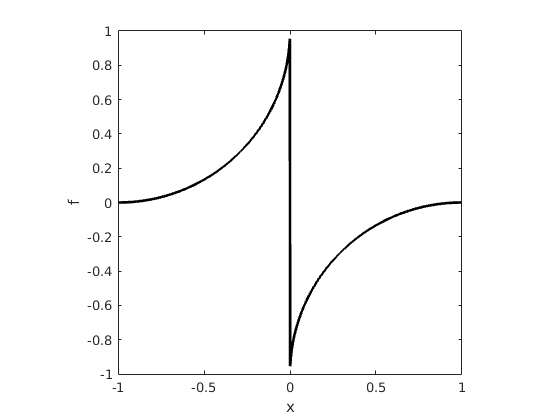
$$f(x)=\begin{cases}x+\frac{a}{2}\\ x-\frac{a}{2}\end{cases}.$$ (18)

If we take

$$\rho_{1}(x)=\rho_{2}(x)=\dfrac{a-\lvert x\rvert}{a^{2}}\quad defined\quad in\quad[-a,a],$$ (19)

we get

$$f(x)=\dfrac{x}{\lvert x\rvert}(\sqrt{2a\lvert x\rvert-x^{2}}-a)\quad on\quad[-a,a]$$ (20)

Figure 1 shows the co-motion functions for (17) and (19).

Figure 1: Right: Co-motion function for (17) with $a=2$. Left: Co-motion function for (19) with $a=1$.

The case $N>2$ and $d=1$

In CPM , the authors proved the existence of optimal transport maps for problem (LABEL:eq6) in dimension $d=1$ and provided an explicit construction of the optimal maps. Let $\rho$ be the normalized electron density and $-\infty=x_{0}<x_{1}<\cdots<x_{N}=+\infty$ be such that

$\int_{x_{i}}^{x_{i+1}}\rho(x)dx=1/N$ $\forall i=0,\cdots,N-1$.

Thus, there exists a unique increasing function $\tilde{f}:\mathbb{R}\rightarrow\mathbb{R}$ on each interval $[x_{i},x_{i+1}]$ such that for every test-function $\varphi$ one has

$$\int_{[x_{i},x_{i+1}]}\varphi(\tilde{f}(x))\rho(x)dx =\int_{[x_{i+1},x_{i+2}]}\varphi(x)\rho(x)dx\quad\forall i=0,\cdots,N-2,$$ (21)

$$\int_{[x_{N-1},x_{N}]}\varphi(\tilde{f}(x))\rho(x)dx =\int_{[x_{0},x_{1}]}\varphi(x)\rho(x)dx,$$ (22)

The optimal maps are then given by

$$f_{2}(x) =\tilde{f}(x)$$ (23)

$$f_{i}(x) =f_{2}^{(i)}(x)\quad\forall i=2,\cdots,N,$$ (24)

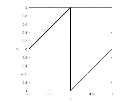
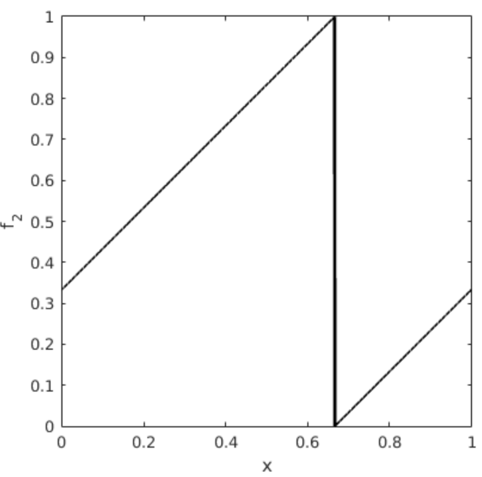
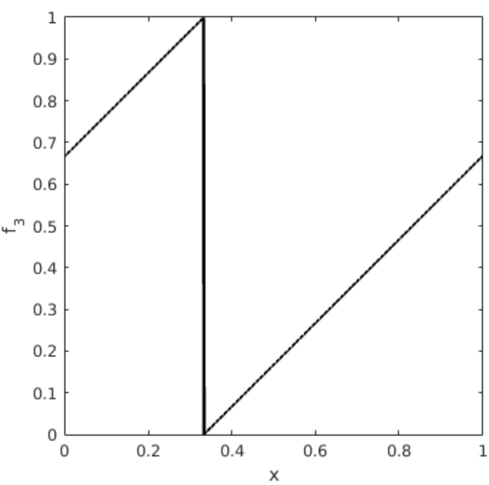
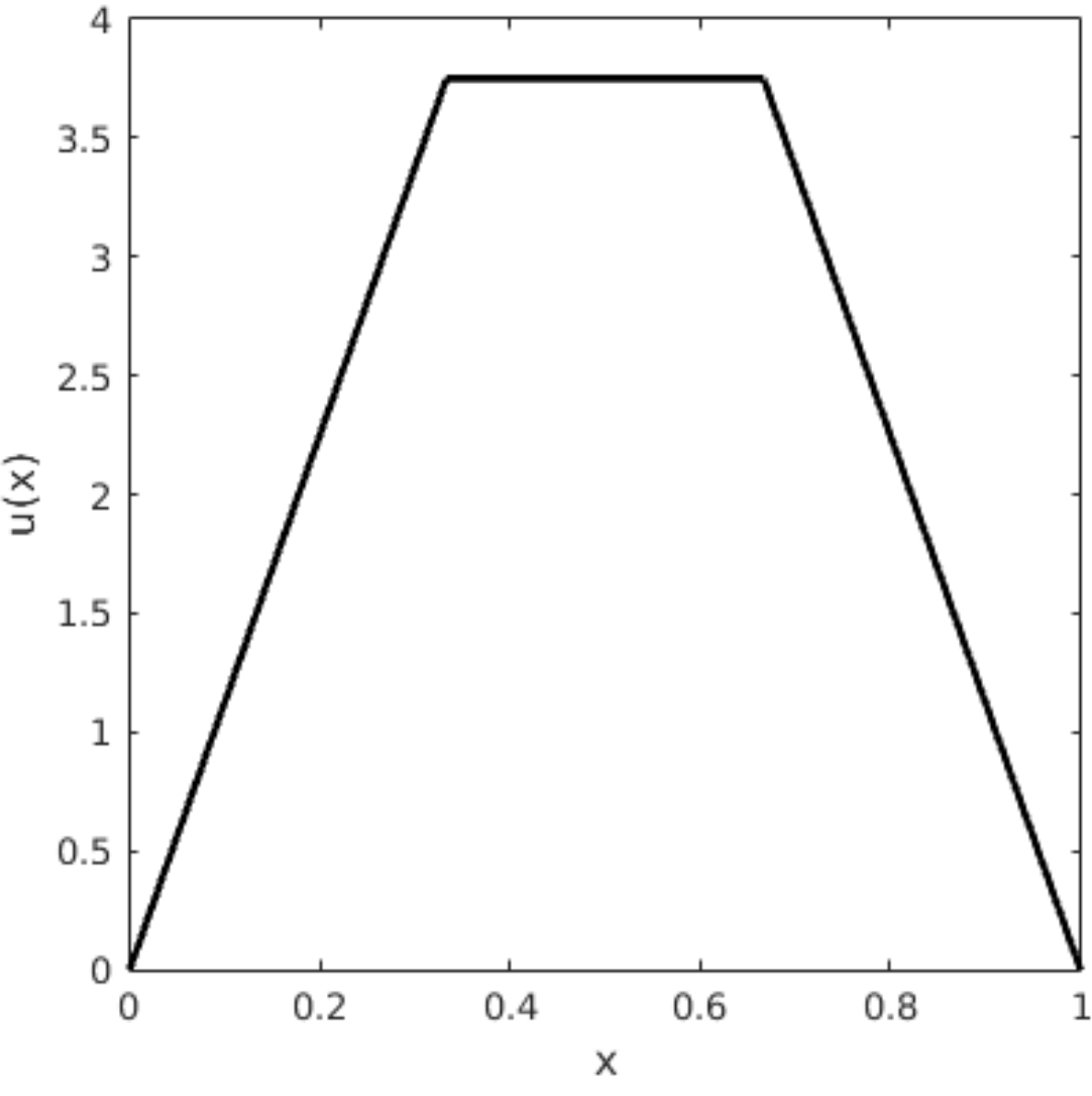
where $f_{2}^{(i)}$ stands for the $i-$th composition of $f_{2}$ with itself. Here, we present an example given in ButDeGo . We consider the case where $\rho$ is the Lebesgue measure on the unit interval $I=[0,1]$, the construction above gives the following optimal co-motion functions

$$\begin{array}[]{l}\mbox{ $f_{2}(x)=\begin{cases}x+1/3\quad if\quad x\leq 2/3\\ x-2/3\quad if\quad x>2/3\end{cases}$, }\\ \mbox{$f_{3}(x)=f_{2}(f_{2}(x))=\begin{cases}x+2/3\quad if\quad x\leq 1/3\\ x-1/3\quad if\quad x>1/3\end{cases}$.}\end{array}$$ (25)

Furthermore, we know that the Kantorovich potential $u$ satisfies the relation (here we take $N=3$)

$$u^{\prime}(x)=-\sum_{i=2}^{N}\dfrac{x-f_{i}(x)}{\lvert x-f_{i}(x)\rvert^{3}}$$ (26)

and by substituting the co-motion functions in (26) (and integrating it) we get

$$u(x)=\begin{cases}\frac{45}{4}x\quad\quad&0\leq x\leq 1/3\\ \frac{15}{4}\quad\quad&1/3\leq x\leq 2/3\\ -\frac{45}{4}x+\frac{45}{4}\quad\quad&2/3\leq x\leq 1\end{cases}$$ (27)

Figure 2 illustrates this example.

When $N\geq 4$ similar arguments as above can be developed and we can similarly compute the co-motion functions and the Kantorovich potential.

Figure 2: Right: co-motion function $f_{2}$ for (25). Center: co-motion function $f_{3}$ for (25). Left: Kantorovich Potential $u(x)$ (27).

The radially symmetric marginal case for $N=2$, $d\geq 2$

We discuss now the radial $d-$dimensional ($d\geq 2$) case for $N=2$. We assume that the marginal $\rho$ is radially symmetric, then we recall the following theorem from CoFrieKl :

Theorem 2.1

CoFrieKl Suppose that $\rho(x)=\rho(\lvert x\rvert)$, then the optimal transport map is given by

$$f^{\star}(x)=\dfrac{x}{\lvert x\rvert}g(|x|),\quad x\in\mathbb{R}^{d},$$ (28)

with $g(r)=-F_{2}^{-1}(F_{1}(r))$, $F_{1}(t):=C(d)\int_{0}^{t}\rho(s)s^{d-1}ds$, $F_{2}(t):=C(d)\int_{t}^{\infty}\rho(s)s^{d-1}ds$ where $C(d)$ denotes the measure of $S^{d-1}$, the unit sphere in $\mathbb{R}^{d}$.

Example 1

(Spherical coordinates system) If $\rho$ is radially symmetric $\rho(x)=\rho(|x|)$, it is convenient to work in spherical coordinates and then to set for every radius $r>0$

$$\lambda(r)=C(d)r^{d-1}\rho(r)$$ (29)

so that for every test-function $\varphi$ we have

$$\int_{\mathbb{R}^{d}}\varphi(x)\rho(|x|)dx=\int_{0}^{+\infty}\Big{(}\int_{S^{d-1}}\varphi(r,\omega)\frac{d\sigma(\omega)}{C_{d}}\Big{)}\lambda(r)dr$$

with $C(d)$ the measure of $S^{d-1}$ and $\sigma$ the $d-1$ measure on $S^{d-1}$ which in particular implies that $\lambda:=|.|_{\#}\rho$ i.e.

$$\int_{\mathbb{R}^{d}}\varphi(|x|)\rho(|x|)dx=\int_{0}^{+\infty}\varphi(r)\lambda(r)dr,\;\forall\varphi\in C_{c}(\mathbb{R}_{+}).$$ (30)

The radial part of the optimal co-motion function $a(r)=-g(r)$ can be computed by solving the ordinary differential equation

$a^{\prime}(r)\lambda(a(r))=\lambda(r)$

which gives

$$\int_{0}^{a(r)}\lambda(s)ds=2-\int_{0}^{r}\lambda(s)ds.$$ (31)

We define $R(r)=\int_{0}^{r}\lambda(s)ds$, since $r\mapsto R(r)$ is increasing, its inverse $R^{-1}(w)$ is well defined for $w\in[0,1)$. Thus, we see that $a(r)$ has the form

$$a(r)=R^{-1}(2-R(r)).$$ (32)

Reducing the dimension under radial symmetry

In the case where the marginal $\rho(x)=\rho(|x|)$ is radially symmetric, the multi-marginal problem with Coulomb cost

$$\inf_{\gamma\in\Pi(\rho,\cdots,\rho)}\int_{\mathbb{R}^{dN}}c(x_{1},\cdots,x_{N})d\gamma(x_{1},\cdots,x_{N})$$ (33)

with $c$ the Coulomb cost given by (11) involves plans on $\mathbb{R}^{dN}$ which is very costly to discretize. Fortunately, thanks to the symmetries of the problem, it can actually be solved by considering a multi-marginal problem only on $\mathbb{R}_{+}^{N}$. Let us indeed define for every $(r_{1},\cdots,r_{N})\in(0,+\infty)^{N}$:

$${\widetilde{c}}(r_{1},\cdots,r_{N}):=\inf\{c(x_{1},\cdots,x_{N})\;:\;|x_{1}|=r_{1},\cdots,|x_{N}|=r_{N}\}.$$ (34)

Defining $\lambda$ by (29) (or equivalently (30)) and defining $\Pi(\lambda,\cdots,\lambda)$ as the set of probability measures on $\mathbb{R}_{+}^{N}$ having each marginal equal to $\lambda$, consider

$$\inf_{{\widetilde{\gamma}}\in\Pi(\lambda,\cdots,\lambda)}\int_{\mathbb{R}_{+}^{N}}{\widetilde{c}}(r_{1},\cdots,r_{N})d{\widetilde{\gamma}}(r_{1},\cdots,r_{N}).$$ (35)

We claim that $\inf(\ref{dftquant})=\inf(\ref{dftquantrad})$. The inequality $\inf(\ref{dftquant})\geq\inf(\ref{dftquantrad})$ is easy: take $\gamma\in\Pi(\rho,\cdots,\rho)$ and define its radial component ${\widetilde{\gamma}}$ by

$$\int_{\mathbb{R}_{+}^{N}}F(r_{1},\cdots,r_{N})d{\widetilde{\gamma}}(r_{1},\cdots,r_{N}):=\int_{\mathbb{R}^{dN}}F(|x_{1}|,\cdots,|x_{N}|)d\gamma(x_{1},\cdots,x_{N}),\;\forall F\in C_{c}(\mathbb{R}_{+}^{N}),$$ (36)

it is obvious that ${\widetilde{\gamma}}\in\Pi(\lambda,\cdots,\lambda)$ and since $c(x_{1},\cdots,x_{N})\geq{\widetilde{c}}(|x_{1}|,\cdots,|x_{N}|)$, the inequality $\inf(\ref{dftquant})\geq\inf(\ref{dftquantrad})$ easily follows. To show the converse inequality, we use duality. Indeed, by standard convex duality, we have

$$\inf(\ref{dftquant})=\sup_{u}\Big{\{}N\int_{\mathbb{R}^{d}}u(x)\rho(x)dx\;:\;\sum_{i=1}^{N}u(x_{i})\leq c(x_{1},\cdots,x_{N})\Big{\}}$$ (37)

and similarly

$$\inf(\ref{dftquantrad})=\sup_{v}\Big{\{}N\int_{\mathbb{R}_{+}}v(r)\lambda(r)dr\;:\;\sum_{i=1}^{N}v(r_{i})\leq{\widetilde{c}}(r_{1},\cdots,r_{N})\Big{\}}.$$ (38)

Now since $\rho$ is radially symmetric and the constraint of (37) is invariant by changing $u$ by $u\circ R$ with $R$ a rotation (see (11)) , there is no loss of generality in restricting the maximization in (37) to potentials of the form $u(x_{i})=w(r_{i})$, but then the constraint of (37) implies that $w$ satisfies the constraint of (38). Then we have $\inf(\ref{dftquant})=\sup(\ref{dualdft})\leq\sup(\ref{dualdftrad})=\inf(\ref{dftquantrad})$. Note then that $\gamma\in\Pi(\rho,\cdots,\rho)$ solves (33) if and only if its radial component ${\widetilde{\gamma}}$ solves (33) and $c(x_{1},\cdots,x_{N})={\widetilde{c}}(|x_{1}|,\cdots,|x_{N}|)$ $\gamma$-a.e. Therefore (33) gives the optimal radial component, whereas the extra condition $c(x_{1},\cdots,x_{N})={\widetilde{c}}(|x_{1}|,\cdots,|x_{N}|)$ $\gamma$-a.e. gives an information on the angular distribution of $\gamma$.

3 Iterative Bregman Projections

Numerics for multi-marginal problems have so far not been extensively developed. Discretizing the multi-marginal problem leads to the linear program (41) where the number of constraints grows exponentially in $N$, the number of marginals. In this section, we present a numerical method which is not based on linear programming techniques, but on an entropic regularization and the so-called alternate projection method. It has recently been applied to various optimal transport problems in CuturiSink and iterative .

The initial idea goes back to von Neumann Ne1 , Ne2 who proved that the sequence obtained by projecting orthogonally iteratively onto two affine subspaces converges to the projection of the initial point onto the intersection of these affine subspaces. Since the seminal work of Bregman bregman , it is by now well-known that one can extend this idea not only to several affine subspaces (the extension to convex sets is due to Dyskstra but we won’t use it in the sequel) but also by replacing the euclidean distance by a general Bregman divergence associated to some suitable strictly and differentiable convex function $f$ (possibly with a domain) where we recall that the Bregman divergence associated with $f$ is given by

$$D_{f}(x,y)=f(x)-f(y)-\langle\nabla f(y),x-y\rangle.$$ (39)

In what follows, we shall only consider the Bregman divergence (also known as the Kullback-Leibler distance) associated to the Boltzmann/Shannon entropy $f(x):=\sum_{i}x_{i}(\log x_{i}-1)$ for non-negative $x_{i}$. This Bregman divergence (restricted to probabilities i.e. imposing the normalization $\sum_{i}x_{i}=1$) is the Kullback-Leibler distance or relative entropy:

$$D_{f}(x,y)=\sum_{i}x_{i}\log\Big{(}\frac{x_{i}}{y_{i}}\Big{)}.$$

Bregman distances are used in many other applications most notably image processing, see osher for instance.

3.1 The Discrete Problem and its Entropic Regularization

In this section we introduce the discrete problem solved using the iterative Bregman projections bregman . From now on, we consider the problem (12)

$$\min_{\gamma_{N}\in\mathcal{C}}\int_{(\mathbb{R}^{d})^{N}}c(x_{1},\cdots,x_{N})\gamma_{N}(x_{1},\cdots,x_{N})dx_{1}\cdots dx_{N},$$ (40)

where $N$ is the number of marginals (or electrons), $c(x_{1},...,x_{N})$ is the Coulomb cost, $\gamma_{N}$ the transport plan, is the probability distribution over $(\mathbb{R}^{d})^{N}$ and $\mathcal{C}:=\bigcap_{i=1}^{N}\mathcal{C}_{i}$ with $\mathcal{C}_{i}:=\{\gamma_{N}\in Prob\{(\mathbb{R}^{d})^{N}\}\lvert\,\pi_{i}\gamma_{N}=\rho\}$ (we remind the reader that electrons are indistinguishable so the $N$ marginals coincide with $\rho$).

In order to discretize (40), we use a discretisation with $M_{d}$ points of the support of the $k$th electron density as $\{x_{j_{k}}\}_{j_{k}=1,\cdots,M_{d}}$. If the densities $\rho$ are approximated by $\sum_{j_{k}}\rho_{j_{k}}\delta_{x_{j_{k}}}$, we get

$$\min_{\gamma\in\mathcal{C}}\sum_{j_{1},\cdots j_{N}}c_{j_{1},\cdots,j_{N}}\gamma_{j_{1},\cdots,j_{N}},$$ (41)

where $c_{j_{1},\cdots,j_{N}}=c(x_{j_{1}},\cdots,x_{j_{N}})$ and the transport plan support for each coordinate is restricted to the points $\{x_{j_{k}}\}_{k}=1,\cdots,M_{d}$ thus becoming a $(M_{d})^{N}$ matrix again denoted $\gamma$ with elements $\gamma_{j_{1},\cdots,j_{N}}$. The marginal constraints $\mathcal{C}_{i}$ becomes

$$\mathcal{C}_{i}:=\{\gamma\in\mathbb{R}_{+}^{(M_{d})^{N}}\lvert\quad\sum_{j_{1},...,j_{i-1},j_{i+1},...,j_{N}}\gamma_{j_{1},...,j_{N}}=\rho_{j_{i}},\,\forall j_{i}=1,\cdots,M_{d}\}.$$ (42)

Recall that the electrons are indistinguishable, meaning that they have same densities : $\rho_{j_{k}}=\rho_{j_{k^{\prime}}},\,\forall j,\,\forall k\neq k^{\prime}$.

The discrete optimal transport problem (41) is a linear program problem and is dual to the discretization of (15)

$$\begin{split}\max_{u_{j}}&\sum_{j=1}^{M}Nu_{j}\rho_{j}\\ s.t.&\sum_{i=1}^{N}u_{j_{i}}\leq c_{j_{1}\cdots j_{N}}\quad\forall j_{i}=1,\cdots,M_{d}\end{split}$$ (43)

where $u_{j}=u_{j_{i}}=u(x_{j_{i}})$. Thus the primal (41) has $(M_{d})^{N}$ unknown and $M_{d}\times N$ linear constraints and the dual (43) only $M_{d}$ unknown but still $(M_{d})^{N}$ constraints. They are computationally not solvable with standard linear programming methods even for small cases in the multi-marginal case.

A different approach consists in computing the problem (41) regularized by the entropy of the joint coupling. This regularization dates to E. Schrödinger Schrodinger31 and it has been recently introduced in machine learning CuturiSink and economics GalichonEntr (we refer the reader to iterative for an overview of the entropic regularization and the iterative Bregman projections in OT). Thus, we consider the following discrete regularized problem

$$\min_{\gamma\in\mathcal{C}}\sum_{j_{1},\cdots j_{N}}c_{j_{1},\cdots,j_{N}}\gamma_{j_{1},\cdots,j_{N}}+\epsilon E(\gamma),$$ (44)

where $E(\gamma)$ is defined as follows

$$E(\gamma)=\begin{cases}\sum_{j_{1},\cdots j_{N}}\gamma_{j_{1},\cdots,j_{N}}\log(\gamma_{j_{1},\cdots,j_{N}})\mbox{ if }\gamma\geq 0\\ +\infty\mbox{ otherwise}.\end{cases}$$ (45)

After elementary computations, we can re-write the problem as

$$\min_{\gamma\in\mathcal{C}}KL(\gamma\lvert\bar{\gamma})$$ (46)

where $KL(\gamma\lvert\bar{\gamma})=\sum_{i_{1},...,i_{N}}\gamma_{i_{1},...,i_{N}}(\log(\dfrac{\gamma_{i_{1},...,i_{N}}}{\bar{\gamma}_{i_{1},...,i{N}}}))$ is the Kullback-Leibler distance and

$$\bar{\gamma}_{i_{1},...,i_{N}}=e^{-\dfrac{c_{j_{1},\cdots,j_{N}}}{\epsilon}}.$$ (47)

As explained in section 1.2, when the transport plan $\gamma$ is concentrated on the graph of a transport map which solves the Monge problem, after discretisation of the densities, this property is lost along but we still expect the $\gamma$ matrix to be sparse. The entropic regularization will spread the support and this helps to stabilize the computation: it defines a strongly convex program with a unique solution $\gamma^{\epsilon}$ which can be obtained through elementary operations (we detail this in section 3.3 for both the continuous and discrete framework). The regularized solutions $\gamma^{\epsilon}$ then converge to $\gamma^{\star}$, the solution of (41) with minimal entropy, as $\epsilon\rightarrow 0$ (see CominettiAsympt for a detailed asymptotic analysis and the proof of exponential convergence). Let us now apply the iterative Bregman projections to find the minimizer of (46).

3.2 Alternate Projections

The main idea of the iterative Bregman projections (we call it Bregman as the Kullback-Leibler distance is also called Bregman distance, see bregman ) is to construct a sequence $\gamma^{n}$ (which converges to the minimizer of (46)) by alternately projecting on each set $\mathcal{C}_{i}$ with respect to the Kullback-Leibler distance. Thus, the iterative KL (or Bregman) projections can be written

$$\begin{cases}\gamma^{0}&=\bar{\gamma}\\ \gamma^{n}&=P_{\mathcal{C}_{n}}^{KL}(\gamma^{n-1})\quad\forall n>0\end{cases}$$ (48)

where we have extended the indexing of the set by $N-$periodicity such that $\mathcal{C}_{n+N}=\mathcal{C}_{n}\quad\forall n\in\mathbb{N}$ and $P_{\mathcal{C}_{n}}^{KL}$ denotes the KL projection on $\mathcal{C}_{n}$.

The convergence of $\gamma^{n}$ to the unique solution of (46) is well known, it actually holds for large classes of Bregman distances and in particular the Kullback-Leibler divergence as was proved by Bauschke and Lewis bauschke-lewis

$\gamma^{n}\rightarrow P_{\mathcal{C}}^{KL}(\bar{\gamma})$ as $n\rightarrow\infty$.

Remark 3

If the convex sets $\mathcal{C}_{i}$ are not affine sub-sets (that is not our case), $\gamma^{n}$ converges toward a point of the intersection which is not the KL projection of $\bar{\gamma}$ anymore so that a correction term is needed as provided by Dykstra’s algorithm (we refer the reader to iterative ).

The KL projection on $\mathcal{C}_{i}\quad i=1,...,N$ can be computed explicitly as detailed in the following proposition

Proposition 1

For $\bar{\gamma}\in(\mathbb{R}_{+})^{{M_{d}}^{N}}$ the projection $P_{\mathcal{C}_{i}}^{KL}(\bar{\gamma})$ is given by

$$P_{\mathcal{C}_{i}}^{KL}(\bar{\gamma})_{j_{1},...,j_{N}}=\rho_{j_{i}}\dfrac{\bar{\gamma}_{j_{1},...,j_{N}}}{\sum_{k_{1},...,k_{i-1},k_{i+1},...,k_{N}}\bar{\gamma}_{k_{1},...,k_{N}}}\quad\forall j_{i}=1,...,M_{d}.$$ (49)

Proof

Introducing Lagrange multipliers $\lambda_{j_{i}}$ associated to the constraint $\mathcal{C}_{i}$

$$\sum_{j_{1},...,j_{i-1},j_{i+1},...,j_{N}}\gamma_{j_{1},...,j_{N}}=\rho_{j_{i}}$$ (50)

the KL projection is given by the optimality condition :

$$\log(\dfrac{\gamma_{j_{1},...,j_{N}}}{\bar{\gamma}_{j_{1},...,j_{N}}})-\lambda_{j_{i}}=0$$ (51)

so that

$$\gamma_{j_{1},...,j_{N}}=C_{j_{i}}\bar{\gamma}_{j_{1},...,j_{N}},$$ (52)

where $C_{j_{i}}=e^{\lambda_{j_{i}}}$. If we substitute (52) in (50), we get

$$C_{j_{i}}=\rho_{j_{i}}\dfrac{1}{\sum_{k_{1},...,k_{i-1},k_{i+1},...,k_{N}}\bar{\gamma}_{k_{1},...,k_{N}}}$$ (53)

which gives (49).

3.3 From the Alternate Projections to the Iterative Proportional Fitting Procedure

The alternate projection procedure (48) is performed on $M_{d}^{N}$ matrices. Moreover each projection (49) involves computing partial sum of this matrix. The total operation cost of each Bregman iteration scales like $O(M_{d}^{2N-1})$.

In order to reduce the cost of the problem, we use an equivalent formulation of the Bregman algorithm known as the Iterative Proportional Fitting Procedure (IPFP). Let us consider the problem (46) in a continous measure setting and, for simplicity, 2-marginals framework

$$\min_{\{\gamma\lvert\pi_{1}(\gamma)=\rho,\pi_{2}(\gamma)=\rho\}}\int\log(\dfrac{d\gamma}{d\bar{\gamma}})d\gamma,$$ (54)

where $\rho$, $\rho$ and $\bar{\gamma}$ are nonnegative measures. The aim of the IPFP is to find the KL projection of $\bar{\gamma}$ on $\Pi(\rho,\rho)$ (see (47) for the definition of $\bar{\gamma}$ which depends on the cost function).

Under the assumption that the value of $(\ref{eq19})$ is finite, Rüschendorf and Thomsen (see RuschendorfThomsen ) proved that a unique KL-projection $\gamma^{*}$ exists and that it is of the form

$$\gamma^{*}(x,y)=a(x)b(y)\bar{\gamma}(x,y),\quad a(x)\geq 0,\quad b(y)\geq 0.$$ (55)

From now on, we consider (with a sligthly abuse of notation) Borel measures with densities $\gamma$, $\bar{\gamma}$, $\rho$ and $\rho$ w.r.t. the suitable Lebesgue measure. $a$ and $b$ can be uniquely determined by the marginal condition as follows

$$\begin{array}[]{ll}a(x)&=\dfrac{\rho(x)}{\int\bar{\gamma}(x,y)b(y)dy},\\ b(y)&=\dfrac{\rho(y)}{\int\bar{\gamma}(x,y)a(x)dx}.\end{array}$$ (56)

Then, IPFP is defined by the following recursion

$b_{0}=1,\quad a_{0}=\rho$,

$$\begin{array}[]{ll}b_{n+1}(y)&=\dfrac{\rho(y)}{\int\bar{\gamma}(x,y)a_{n}(x)dx},\\ a_{n+1}(x)&=\dfrac{\rho(x)}{\int\bar{\gamma}(x,y)b_{n+1}(y)dy}.\end{array}$$ (57)

Moreover, we can define the sequence of joint densities (and of the corresponding measures)

$$\gamma^{2n}(x,y):=a^{n}(x)b^{n}(y)\bar{\gamma}(x,y)\quad\gamma^{2n+1}:=a^{n}(x)b^{n+1}(y)\bar{\gamma}(x,y),\quad n\geq 0.$$ (58)

Rüschendorf proved (see Ruschendorf95 ) that $\gamma^{n}$ converges to the KL-projection of $\bar{\gamma}$. We can, now, recast the IPFP in a discrete framework, which reads as

$$\gamma_{ij}=a_{i}b_{j}\bar{\gamma}_{ij},\; b_{j}^{0}=1,\quad a_{i}^{0}=\rho_{i},$$ (59)

$$\begin{array}[]{ll}b_{j}^{n+1}&=\dfrac{\rho_{j}}{\sum_{i}\bar{\gamma}_{ij}a_{i}^{n}},\\ a_{i}^{n+1}&=\dfrac{\rho_{i}}{\sum_{j}\bar{\gamma}_{ij}b_{j}^{n+1}},\end{array}$$ (60)

$$\gamma_{ij}^{2n}=a_{i}^{n}\bar{\gamma}_{ij}b_{j}^{n}\quad\gamma_{ij}^{2n+1}=a_{i}^{n}\bar{\gamma}_{ij}b_{j}^{n+1}.$$ (61)

By definition of $\gamma_{ij}^{n}$, notice that

$\bar{\gamma}_{ij}b_{j}^{n}=\dfrac{\gamma_{ij}^{2n-1}}{a_{i}^{n-1}}$ and $a_{i}^{n}\bar{\gamma}_{ij}=\dfrac{\gamma_{ij}^{2n}}{b_{j}^{n}}$

and if (61) is re-written as follows

$$\begin{array}[]{ll}\gamma_{ij}^{2n}&=\rho_{i}\dfrac{\bar{\gamma}_{ij}b_{j}^{n}}{\sum_{k}\bar{\gamma}_{ik}b_{k}^{n}}\\ \gamma_{ij}^{2n+1}&=\rho_{j}\dfrac{\bar{\gamma}_{ij}a_{i}^{n}}{\sum_{k}\bar{\gamma}_{kj}a_{k}^{n}}\end{array}$$ (62)

then we obtain

$$\begin{array}[]{ll}\gamma_{ij}^{2n}&=\rho_{i}\dfrac{\gamma_{ij}^{2n-1}}{\sum_{k}\gamma_{ik}^{2n-1}}\\ \gamma_{ij}^{2n+1}&=\rho_{j}\dfrac{\gamma_{ij}^{2n}}{\sum_{k}\gamma_{kj}^{2n}}.\end{array}$$ (63)

Thus, we exactly recover the Bregman algorithm described in the previous section, for 2 marginals.

The extension to the multi-marginal framework is straightforward but cumbersone to write. It leads to a problem set on $N$ $M_{d}$-dimensional vectors $a_{j,i_{(\cdot)}},\quad\,j=1,\cdots,N,\quad i_{(\cdot)}=1,\cdots,M_{d}$. Each update takes the form

$$a_{j,i_{j}}^{n+1}=\dfrac{\rho_{i_{j}}}{\sum_{i_{1},i_{2},...i_{j-1},i_{j+1},...,i_{N}}\bar{\gamma}_{i_{1},...,i_{N}}\,a_{1,i_{1}}^{n+1}\,a_{2,i_{2}}^{n+1}...a_{j-1,i_{j-1}}^{n+1}\,a_{j+1,i_{j+1}}^{n}...a_{N,{i_{N}}}^{n}\,},$$ (64)

Where each $i_{k}$ takes values in $\{1,\cdots,M_{d}\}$.

Note that we still need a constant $M_{d}^{N}$ cost matrix $\bar{\gamma}$. Thanks to the symmetry and separability properties of the cost function (see (11) and (47)) , it is possible to replace it by a $N\,(N-1)/2$ product of $M_{d}^{2}$ matrices. This is already a big improvement from the storage point of view. Further simplifications are under investigations but the brute force IPFP operational cost therefore scales like $O(N\,M_{d}^{N+1})$ which provides a small improvement over the Bregman iterates option.

3.4 A heuristic refinement mesh strategy

We will use a heuristic refinement mesh strategy allowing to obtain more accuracy without increasing the computational cost and memory requirements. This idea was introduced in oberman for the adaptative resolution of the pure Linear Programming formulation of the Optimal Transportation problem, i.e without the entropic regularisation.

If the optimal transport plan is supported by a lower dimensional set, we expect the entropic regularisation to be concentrated on a mollified version of this set. Its width should decrease with the entropic parameter $\epsilon$ if the discretisation is fine enough. Working with a fixed $\epsilon$, the idea is to apply coarse to fine progressive resolution and work with a sparse matrix $\gamma$. At each level, values below a threshold are filtered out (set to 0), then new positive values are interpolated on a finer grid (next level) where $\gamma$ is strictly positive.

To simplify the exposition, we describe the algorithm for $2-$marginals in $1D$ and take a $\sqrt{M}$ gridpoints discretization of $I=[a,b]\in\mathbb{R}$:

1. we start with a cartesian $M$ gridpoints mesh on $I\times I$ to approximate transport plan $\gamma^{\epsilon}$, obtained by running the IPFP on a coarse grid.

2. we take $m_{c}(j)=max_{i}\gamma^{\epsilon}_{ij}$ and $m_{r}(i)=max_{j}\gamma^{\epsilon}_{ij}$ which are the maximum values over the rows and over the columns respectively, and we define

   $m=\min[\min_{j}(m_{c}(j)),\min_{i}(m_{r}(i))]$.

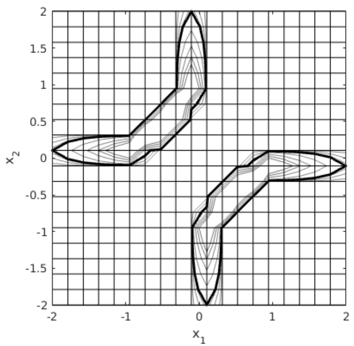
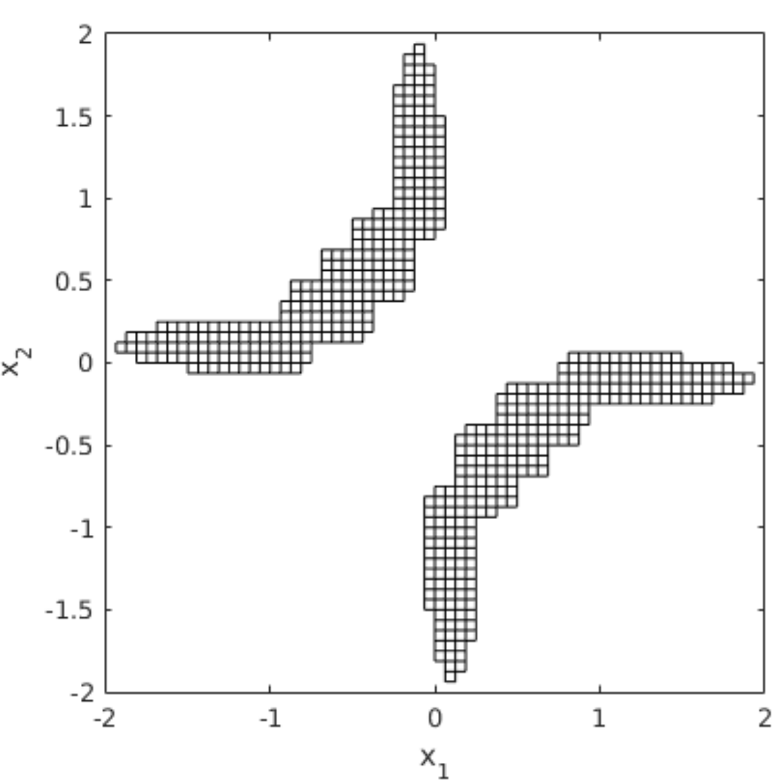
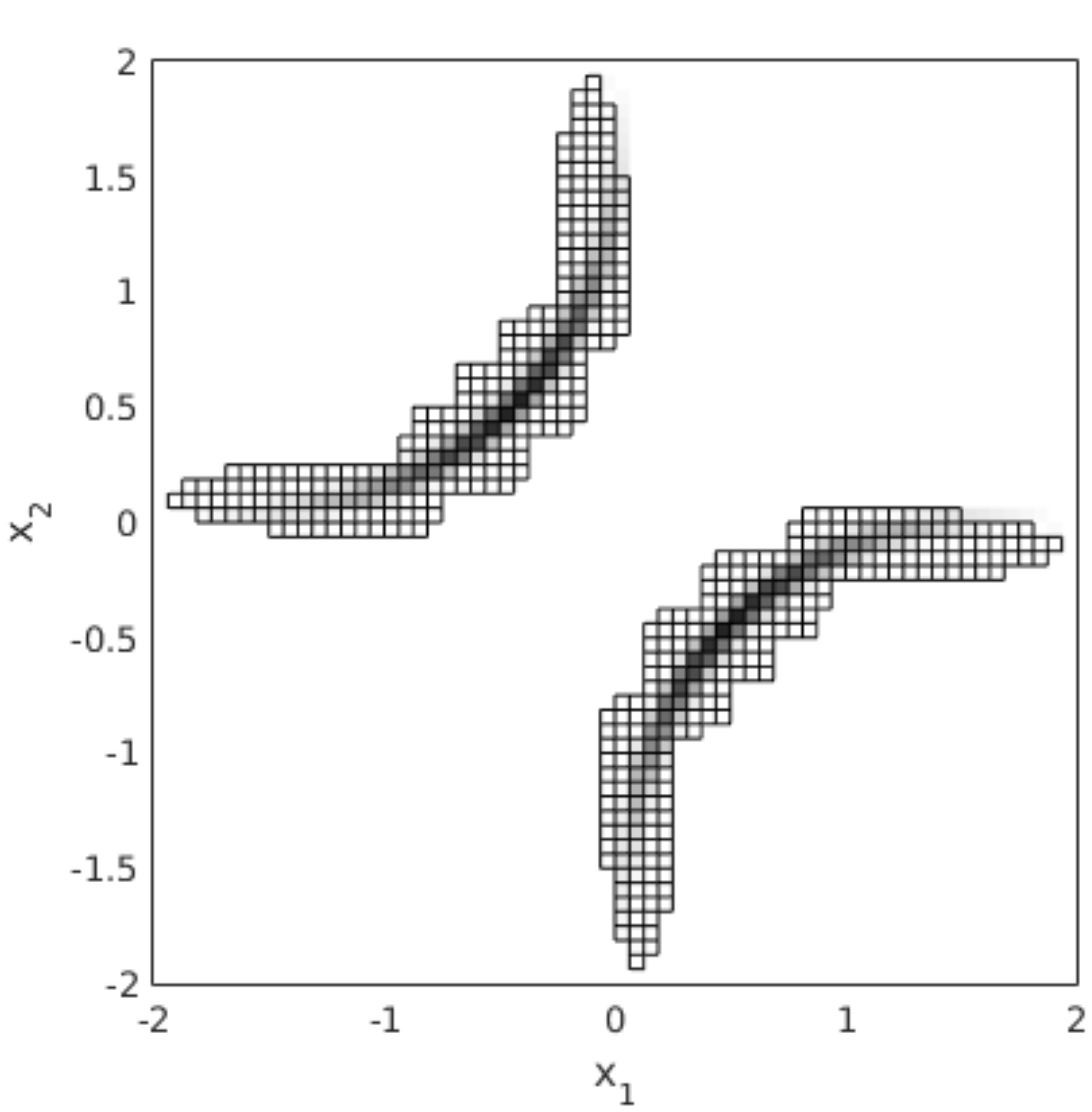
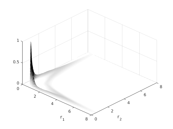
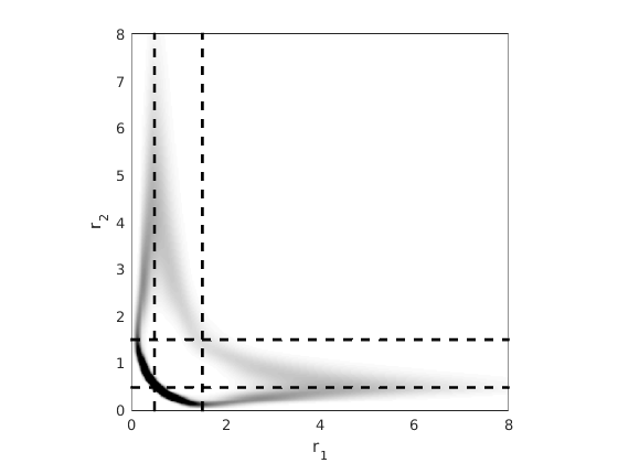
   We will refine the grid only inside the level curve $\gamma^{\epsilon}=\xi m$ where we expect the finer solution is supported, see figure 3.

3. In order to keep approximately the same number of element in the sparse matrix $\gamma$ at each level we refine the grid as follows : Let $\mathcal{T}:=\{(i,j)\lvert\gamma^{\epsilon}_{ij}\geq\xi m\}$ and $M_{\mathcal{T}}:=\sharp\mathcal{T}$ and $r:=M_{\mathcal{T}}/M$, then the size of the grid at the next level is $M^{new}=M/r$.
   

4. We compute the interpolation $\gamma_{M^{new}}$ of the old transport plan $\gamma_{M}$ on the finer grid.

5. Elements of $\gamma_{M^{new}}$ below the fixed threshold $\xi m$ are filtered out, i.e are fixed to $0$ and are not used in the IPFP sum computations, see figure 3.

6. Finally, a new IPFP computation is performed and it can be initialised with an interpolation of the data at the previous level ($\bar{\gamma}$ can be easly re-computed on the gridpoints where $\gamma_{M^{new}}$ is strictly positive).

Figure 3: Left: $\mathcal{T}$ is the set of grid points inside the level curve $\gamma=\xi\,m$ ($\xi=0.9$) (the bold line curve). Center: The new grid after the refinement. Right: The transport Plan after a new IPFP computation

4 Numerical Results

4.1 $N=2$ electrons: comparison between numerical and analytical results

In order to validate the numerical method, we now compare some numerical results for $2$ electrons in dimension $d=1,\cdots,3$ with the analytical results from section 2.2. Let us first consider a uniform density (as (17) with $a=2$) in $1D$. In table 1, we analyze the performance of the numerical method by varying the parameter $\epsilon$. We notice that the error becomes smaller by decreasing the regularizing parameter, but the drawback is that the method needs more iterations to converge. 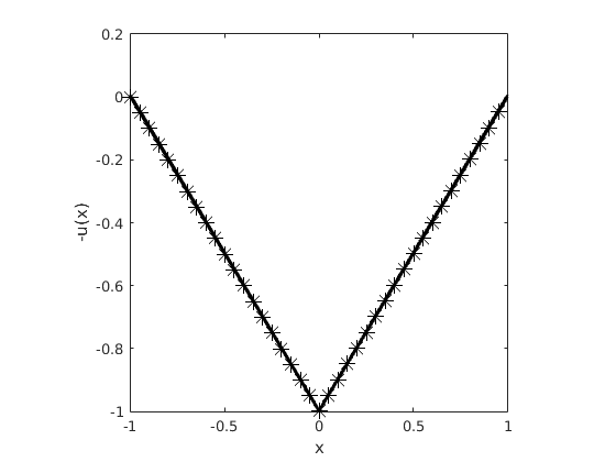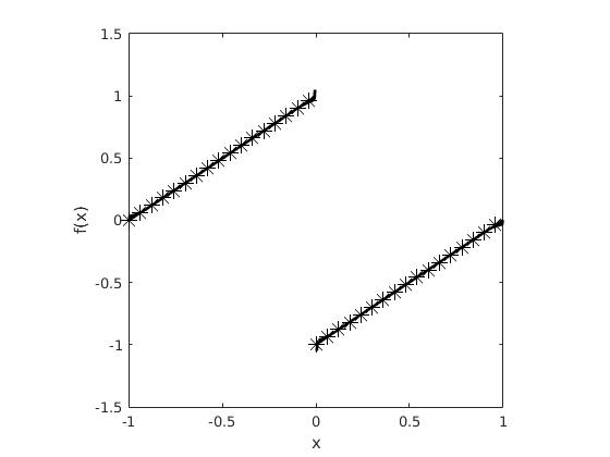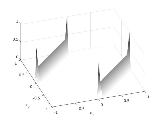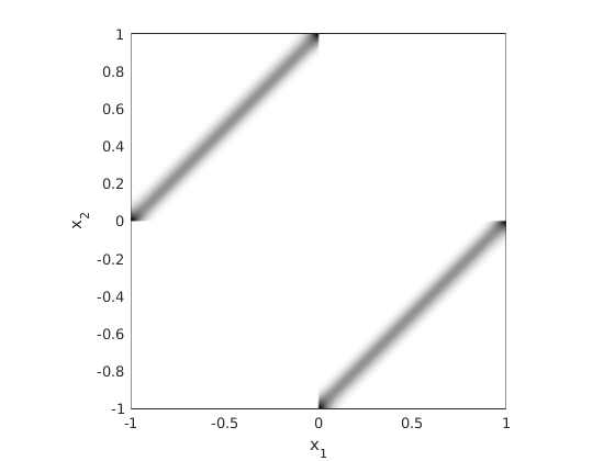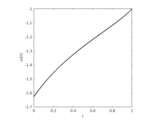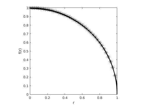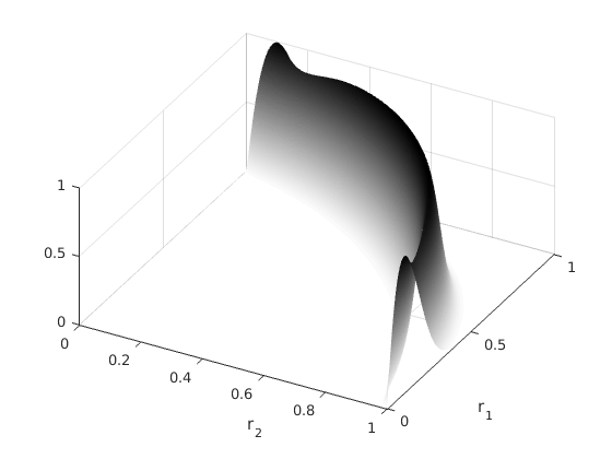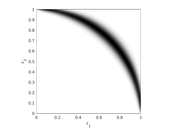Figure 4 shows the Kantorovich potential, the co-motion function which can be recovered from the potential by using (16) and the transport plan. The simulation is performed with a discretization of (17) with $a=2$, $M=1000$ (gridpoints) and $\epsilon=0.004$.

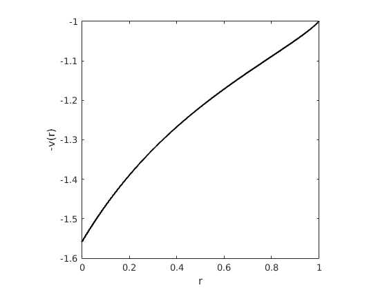
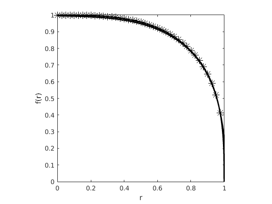
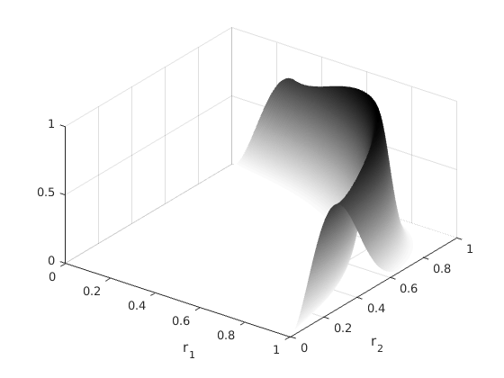
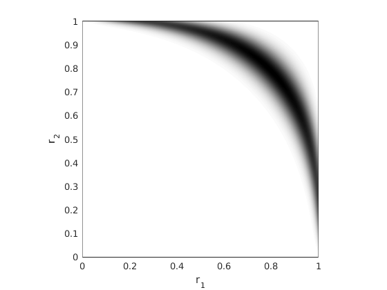
As explained in section 2.2, we can also compute the co-motion for a radially symmetric density. We have tested the method in $2D$ and $3D$, figure 5 and 6 respectively, by using the normalized uniform density on the unit ball. Moreover, in the radial case we have proved that the OT problem can be reduced to a $1-$dimensional problem by computing ${\widetilde{c}}$ which is trivial for the $2$ electrons case: let us set the problem in $2D$ in polar coordinates $(r_{1},\theta_{1})$ and $(r_{2},\theta_{2})$, for the first and the second electron respectively (without loss of generality we can set $\theta_{1}=0$), then it is easy to verify that the minimum is achieved with $\theta_{2}=\pi$. Figure 5 shows the Kantorovich potential (the radial component $v(r)$ as defined in section 2.2), the co-motion and the transport plan for the $2-$dimensional case, the simulation is performed with $M=1000$ and $\epsilon=0.002$. In figure 6 we present the result for th $3-$dimensional case, the simulation is performed with $M=1000$ and $\epsilon=0.002$.

Remark 4

One can notice that, in the case of a uniform density, the transport plan presents a concentration of mass on the boundaries. This is a combined effect of the regularization and of the fact that the density has a compact support.

$\epsilon$	Error ($\lVert u^{\epsilon}-u\rVert_{\infty}/\lVert u\rVert_{\infty}$)	Iteration
0.256	0.1529	11
0.128	0.0984	16
0.064	0.0578	25
0.032	0.0313	38
0.016	0.0151	66
0.008	0.0049	114
0.004	0.0045	192

Table 1: Numerical results for uniform density in 1D. $u^{\epsilon}$ is the numerical Kantorovich potential and $u$ is the analytical one.

Figure 4: Top-Left: Kantorovich Potential $u(x)$. Top-Right: Numerical co-motion function (solid line) and analytical co-motion (star-solid line) . Bottom-Left: Transport plan $\tilde{\gamma}$. Bottom-Right: Support of $\tilde{\gamma}$.

Figure 5: Top-Left: Kantorovich Potential $v(r)$. Top-Right: Numerical co-motion function (solid line) and analytical co-motion (star-solid line) . Bottom-Left: Transport plan $\tilde{\gamma}$. Bottom-Right: Support of $\tilde{\gamma}$.

Figure 6: Top-Left: Kantorovich Potential $v(r)$. Top-Right: Numerical co-motion function (solid line) and analytical co-motion (star-solid line) . Bottom-Left: Transport plan $\tilde{\gamma}$. Bottom-Right: Support of $\tilde{\gamma}$.

4.2 $N=2$ electrons in dimension $d=3$ : Helium atom

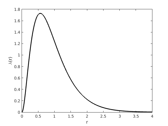
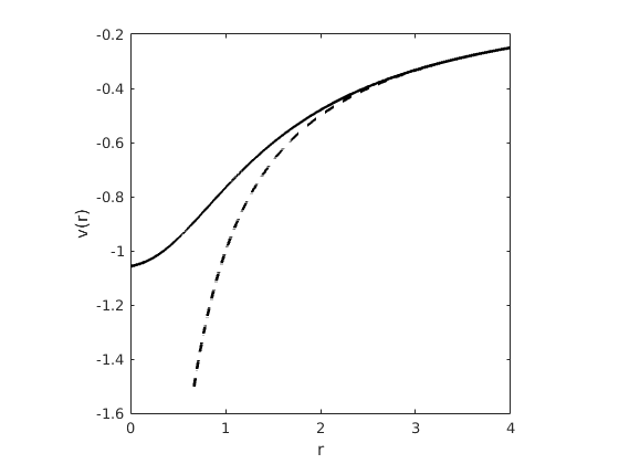
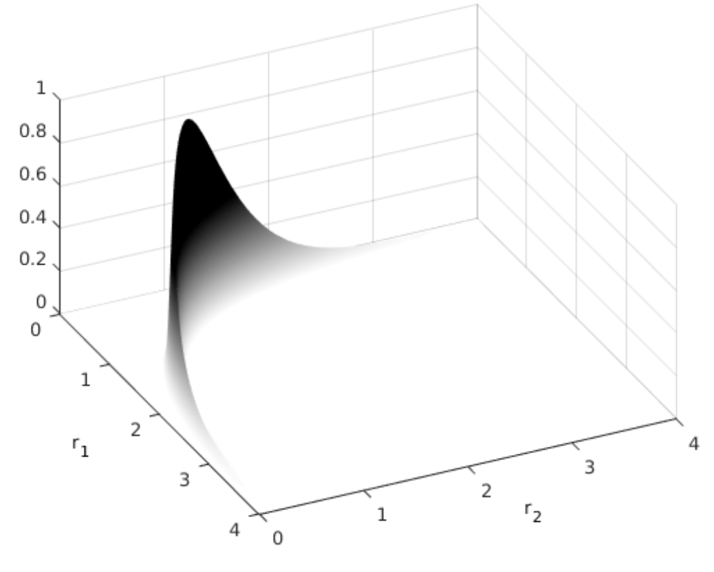
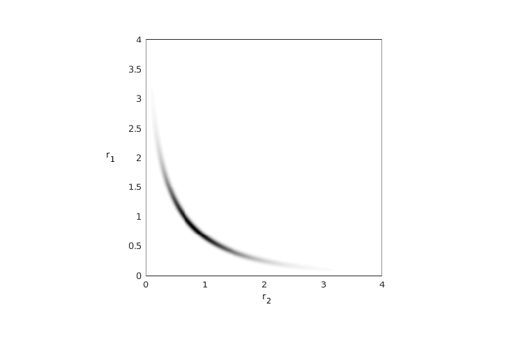
Once we have validated the method with some analytical examples, we solve the regularized problem for the Helium atom by using the electron density computed in Helium . In figure 7, we present the electron density, the Kantorovich potential and the transport plan. The simulation is performed with a discretization of $[0,4]$ with $M=1000$ and $\epsilon=5\,10^{-3}$. We can notice the potential correctly fits the asymptotic behaviour from SeidlGoriSavin , namely $v(r)\sim\dfrac{N-1}{\lvert r\rvert}$ for $r\rightarrow\infty$, where $N$ is the number of electrons.

Figure 7: Top-Left: Helium density $\lambda(r)=4\pi r^{2}\rho(r)$. Top-Right: Kantorovich Potential $v(r)$ (blue) and asymptotic behaviour (red) $v(r)\sim\frac{1}{r}\quad r\rightarrow\infty$. Bottom-Left: Transport plan $\tilde{\gamma}$. Bottom-Right: Support of $\tilde{\gamma}$. All quantities are in Hartree atomic units.

4.3 $N=3$ electrons in dimension $d=1$

We present now some results for the $1-$dimensional multi-marginal problem with $N=3$. They are validated against the analytical solutions given in section 2.2. We recall that splitting $\rho$ into three tertiles $\rho_{i}$ with equal mass, we will have $\rho_{1}\rightarrow\rho_{2}$, $\rho_{2}\rightarrow\rho_{3}$ and $\rho_{3}\rightarrow\rho_{1}$.

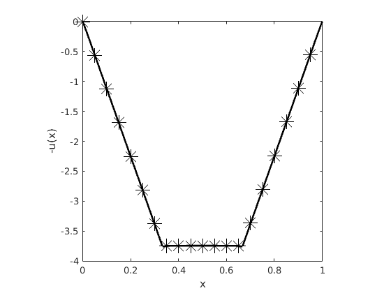
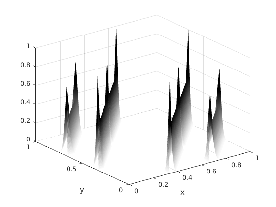
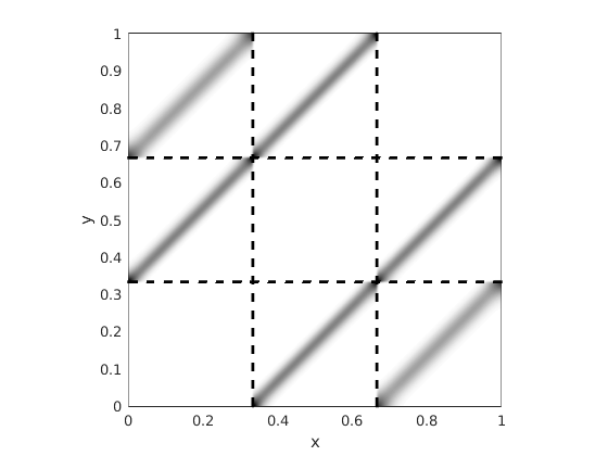
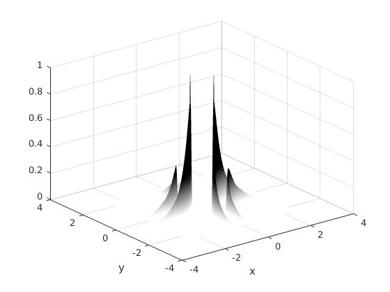
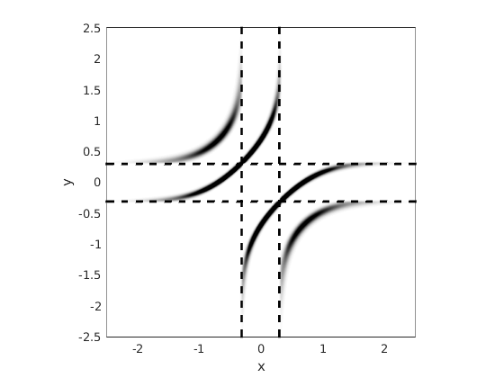
In table 2, we present the perfomance of the method for a uniform density on $[0,1]$ by varying $\epsilon$ and, as expected, we see the same behaviour as in the $2$ marginals case. Figure 8 shows the Kantorovich potential and the projection of the transport plan onto two marginals (namely $\gamma^{2}=\pi_{12}(\gamma^{\epsilon})$). The support gives the relative positions of two electrons.

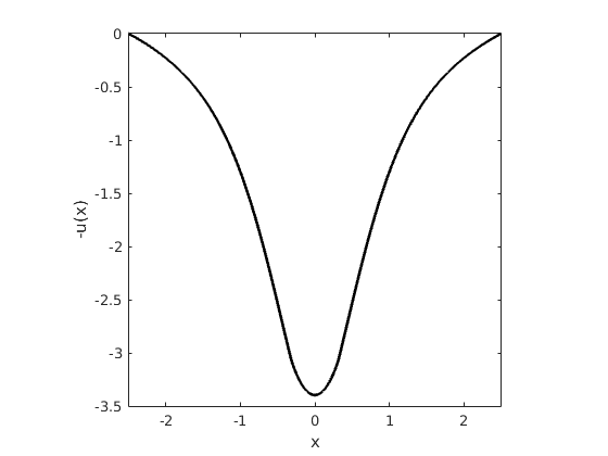
The simulation is performed on a discretization of $[0,1]$ with a uniform density, $M=1000$ and $\epsilon=0.02$. If we focus on the support of the projected transport plan we can notice that the numerical solution correctly reproduces the prescribed behavior The concentration of mass is again due to the compact support of the density, which is not the case of the gaussian as one can see in figure 9. In figure 9 we present the numerical results for $\rho(x)=e^{-x^{2}}/\sqrt{\pi}$. The simulation is performed on the discretization of $[-2.5,2.5]$ with $M=1000$ and $\epsilon=0.008$.

$\epsilon$	Error ($\lVert u^{\epsilon}-u\rVert_{\infty}/\lVert u\rVert_{\infty}$)	Iteration
0.32	0.0658	121
0.16	0.0373	230
0.08	0.0198	446
0.04	0.0097	878
0.02	0.0040	1714

Table 2: Numerical results for uniform density in 1D and three electrons. $u^{\epsilon}$ is the numerical Kantorovich potential and $u$ is the analytical one.

Figure 8: Left: Numerical Kantorovich potential $u(x)$ (solid line) and analytical potential (star-solid line). Center: Projection of the transport plan $\pi_{12}(\gamma(x,y,z))$. Rigth: Support of $\pi_{12}(\gamma(x,y,z))$ The dot-dashed lines delimit the intervals where $\rho_{i}$, with $i=1,\cdots,3$, are defined.

Figure 9: Left: Kantorovich potential $u(x)$. Center: Projection of the transport plan $\pi_{12}(\gamma(x,y,z))$. Rigth: Support of $\pi_{12}(\gamma(x,y,z))$. The dot-dashed lines delimit the intervals where $\rho_{i}$, with $i=1,\cdots,3$, are defined.

4.4 $N=3$ electrons in dimension $d=3$ radial case : Litium atom

We finally perform some simulations for the radial $3-$dimensional case for $N=3$. As for the $3-$dimensional case with $2$ marginals we solve the reduced problem: let us consider the spherical coordinates $(r_{i},\theta_{i},\phi_{i})$ with $i=1,\cdots,3$ and we fix $\theta_{1}=0$ and $\phi_{1}=\phi_{2}=0$ (the first electrons defines the z axis and the second one is on the xz plane). We then notice that $\phi_{3}=0$ as the electrons must be on the same plane of the nucleus to achieve compensation of forces (one can see it by computing the optimality conditions), so we have to minimize on $\theta_{2}$ and $\theta_{3}$ in order to obtain ${\widetilde{c}}$.

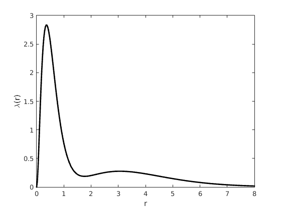
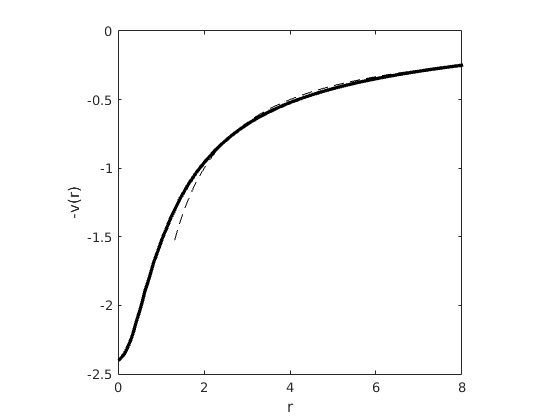
Figure 10 shows the electron density of the Litium (computed in litium ), the Kantorovich Potential (and the asymptotic behavior) and the projection of the transport plan onto two marginals $\tilde{\gamma}^{2}=\pi_{12}(\tilde{\gamma}^{\epsilon})$. The support gives the relative positions of two electrons.

The simulation is performed on a discretization of $[0,8]$ with $M=300$ and $\epsilon=0.007$. Our results show (taking into account the regularization effect) a concentrated transport plan for this kind of density and they match analogous result obtained in SeidlGoriSavin . If we focus on the support of the transport plan we can notice that the optimal solution forces the electrons to occupy three different regions as conjectured in SeidlGoriSavin .

Figure 10: Top-Left: Litium density $\lambda(r)=4\pi r^{2}\rho(r)$. Top-Right: Kantorovich Potential $v(r)$ (blue) and asymptotic behaviour (red) $v(r)\sim\frac{2}{r}\quad r\rightarrow\infty$. Bottom-Left: Projection of the Transport plan $\tilde{\gamma}^{2}=\pi_{12}(\tilde{\gamma}^{\epsilon})$. Bottom-Right: Support of the projected transport plan $\tilde{\gamma}^{2}$. The dot-dashed lines delimit the three regions that the electrons must occupy, we computed them numerically following the idea in SeidlGoriSavin .All quantities are in Hartree atomic units.

5 conclusion

We have presented a numerical scheme for solving multi-marginal OT problems arising from DFT. This is a challenging problems, not only because of the unusual features of the Coulomb cost which is singular and repulsive but also due to the high dimension of the space of plans.

Using an entropic regularization gives rise to a Kullback-Leibler projection problem onto the intersection of affine subsets given by the marginal constraints. Because each projection is explicit, one can use Bregman’s iterative projection algorithm to approximate the solution.

The power of such an iterative projection approach was recently emphasized in CuturiSink ; iterative for the entropic regularization of optimal transport problems, we showed that is also well suited to treat the multi-marginal OT problem with Coulomb cost and leads to the same benefits in terms of convexification of the problem and simplicity of implemention.

The method presented here is just a preliminary step which is simple to implement and therefore easy to use in practice. The cost of solving the general DFT problem in dimension 3 for a large number of electrons is still unfeasible and we need to use radial symmetry simplification and also a heuristic refinement mesh strategy.

A lot of questions are left for future research : can IPFP be used for sharper approximations for DFT? Can one justify rigorously and quantitatively the mesh refinement strategy? How should the regularization parameter $\varepsilon$ be chosen in practice? Does the entropic regularization have a physical interpretation?

References

- (1) Bauschke, H.H., Lewis, A.S.: Dykstra’s algorithm with Bregman projections: a convergence proof. Optimization 48(4), 409–427 (2000)
- (2) Benamou, J.D., Carlier, G., Cuturi, M., Nenna, L., Peyré, G.: Iterative bregman projections for regularized transportation problems. arXiv preprint arXiv:1412.5154 (2014)
- (3) Bregman, L.M.: The relaxation method of finding the common point of convex sets and its application to the solution of problems in convex programming. USSR computational mathematics and mathematical physics 7(3), 200–217 (1967)
- (4) Brenier, Y.: Polar factorization and monotone rearrangement of vector-valued functions. Comm. Pure Appl. Math. 44(4), 375–417 (1991). DOI 10.1002/cpa.3160440402. URL http://dx.doi.org/10.1002/cpa.3160440402
- (5) Bunge, C.: The full ci density of the li atom has been computed with a very large basis set with 8 s functions and up to k functions. private communication
- (6) Buttazzo, G., De Pascale, L., Gori-Giorgi, P.: Optimal-transport formulation of electronic density-functional theory. Phys. Rev. A 85, 062,502 (2012). DOI 10.1103/PhysRevA.85.062502. URL http://link.aps.org/doi/10.1103/PhysRevA.85.062502
- (7) Carlier, G., Ekeland, I.: Matching for teams. Econom. Theory 42(2), 397–418 (2010). DOI 10.1007/s00199-008-0415-z. URL http://dx.doi.org/10.1007/s00199-008-0415-z
- (8) Colombo, M., De Pascale, L., Di Marino, S.: Multimarginal optimal transport maps for one-dimensional repulsive costs. Canad. J. Math. 67, 350–368 (2015)
- (9) Cominetti, R., Martin, J.S.: Asymptotic analysis of the exponential penalty trajectory in linear programming. Mathematical Programming 67(1-3), 169–187 (1994)
- (10) Cotar, C., Friesecke, G., Klüppelberg, C.: Density functional theory and optimal transportation with Coulomb cost. Communications on Pure and Applied Mathematics 66(4), 548–599 (2013). DOI 10.1002/cpa.21437. URL http://dx.doi.org/10.1002/cpa.21437
- (11) Cotar, C., Friesecke, G., Pass, B.: Infinite-body optimal transport with coulomb cost. Calculus of Variations and Partial Differential Equations pp. 1–26 (2013)
- (12) Cuturi, M.: Sinkhorn distances: Lightspeed computation of optimal transport. In: Advances in Neural Information Processing Systems (NIPS) 26, pp. 2292–2300 (2013)
- (13) Freund, D.E., Huxtable, B.D., Morgan, J.D.: Variational calculations on the helium isoelectronic sequence. Phys. Rev. A 29, 980–982 (1984). DOI 10.1103/PhysRevA.29.980. URL http://link.aps.org/doi/10.1103/PhysRevA.29.980
- (14) Friesecke, G., Mendl, C.B., Pass, B., Cotar, C., Klüppelberg, C.: N-density representability and the optimal transport limit of the hohenberg-kohn functional. The Journal of chemical physics 139(16), 164,109 (2013)
- (15) Galichon, A., Salanié, B.: Matching with trade-offs: Revealed preferences over competing characteristics. Tech. rep., Preprint SSRN-1487307 (2009)
- (16) Gangbo, W., Świȩch, A.: Optimal maps for the multidimensional Monge-Kantorovich problem. Comm. Pure Appl. Math. 51(1), 23–45 (1998). DOI 10.1002/(SICI)1097-0312(199801)51:1<23::AID-CPA2>3.0.CO;2-H. URL http://dx.doi.org/10.1002/(SICI)1097-0312(199801)51:1<23::AID-CPA2>3.0.CO;2-H
- (17) Ghoussoub, N., Maurey, B.: Remarks on multi-marginal symmetric Monge-Kantorovich problems. Discrete Contin. Dyn. Syst. 34(4), 1465–1480 (2014)
- (18) Goldstein, T., Bresson, X., Osher, S.: Geometric applications of the split bregman method: Segmentation and surface reconstruction. Journal of Scientific Computing 45(1-3), 272–293 (2010). DOI 10.1007/s10915-009-9331-z. URL http://dx.doi.org/10.1007/s10915-009-9331-z
- (19) Hohenberg, P., Kohn, W.: Inhomogeneous electron gas. Phys. Rev. 136, B864–B871 (1964). DOI 10.1103/PhysRev.136.B864. URL http://link.aps.org/doi/10.1103/PhysRev.136.B864
- (20) Kantorovich, L.: On the transfer of masses (in russian). Doklady Akademii Nauk 37(2), 227–229 (1942)
- (21) Kohn, W., Sham, L.J.: Self-consistent equations including exchange and correlation effects. Phys. Rev. 140, A1133–A1138 (1965). DOI 10.1103/PhysRev.140.A1133. URL http://link.aps.org/doi/10.1103/PhysRev.140.A1133
- (22) Malet, F., Gori-Giorgi, P.: Strong correlation in kohn-sham density functional theory. Phys. Rev. Lett. 109, 246,402 (2012). DOI 10.1103/PhysRevLett.109.246402. URL http://link.aps.org/doi/10.1103/PhysRevLett.109.246402
- (23) Mendl, C.B., Lin, L.: Kantorovich dual solution for strictly correlated electrons in atoms and molecules. Physical Review B 87(12), 125,106 (2013)
- (24) Monge, G.: Mémoire sur la théorie des déblais et des remblais. De l’Imprimerie Royale (1781)
- (25) von Neumann, J.: Functional Operators. Vol. 1: Measures and integrals. Vol 2: The geometry of orthogonal spaces. 21, 22 (1950–1951)
- (26) Neumann, J.V.: On rings of operators. reduction theory. Annals of Mathematics 50(2), pp. 401–485 (1949). URL http://www.jstor.org/stable/1969463
- (27) Oberman, A.: private communication. paper in preparation
- (28) Pass, B.: Uniqueness and Monge solutions in the multimarginal optimal transportation problem. SIAM Journal on Mathematical Analysis 43(6), 2758–2775 (2011). DOI 10.1137/100804917. URL http://link.aip.org/link/?SJM/43/2758/1
- (29) Pass, B.: Multi-marginal optimal transport and multi-agent matching problems: uniqueness and structure of solutions. Discrete Contin. Dyn. Syst. 34(4), 1623–1639 (2014). DOI 10.3934/dcds.2014.34.1623. URL http://dx.doi.org/10.3934/dcds.2014.34.1623
- (30) Ruschendorf, L.: Convergence of the iterative proportional fitting procedure. The Annals of Statistics 23(4), 1160–1174 (1995)
- (31) Ruschendorf, L., Thomsen, W.: Closedness of sum spaces and the generalized Schrodinger problem. Theory of Probability and its Applications 42(3), 483–494 (1998)
- (32) Schrodinger, E.: Uber die umkehrung der naturgesetze. Sitzungsberichte Preuss. Akad. Wiss. Berlin. Phys. Math. 144, 144–153 (1931)
- (33) Seidl, M., Gori-Giorgi, P., Savin, A.: Strictly correlated electrons in density-functional theory: A general formulation with applications to spherical densities. Phys. Rev. A 75, 042,511 (2007). DOI 10.1103/PhysRevA.75.042511. URL http://link.aps.org/doi/10.1103/PhysRevA.75.042511
- (34) Villani, C.: Topics in Optimal Transportation. Graduate Studies in Mathematics Series. American Mathematical Society (2003). URL http://books.google.fr/books?id=GqRXYFxe0l0C
- (35) Villani, C.: Optimal transport: old and new, vol. 338. Springer (2009)