Abstract

In this paper, we perform a comprehensive study to probe the effects of large extra dimensions through double Higgs production in proton-proton collisions at the center-of-mass energies of 14, 33, 100 TeV. We concentrate on the channel in which both Higgs bosons decay into $b\bar{b}$ pair and take into account the main background contributions through realistic Monte-Carlo simulations. In order to achieve an efficient event reconstruction and a good background rejection, jet substructure techniques are used to efficiently capture the boosted Higgs bosons in the final state. The expected limits on the model parameters are obtained based on the invariant mass and the angular properties of the final state objects. Depending on the number of extra dimensions, bounds up to 6.1, 12.5, 28.1 TeV are set on the model parameter at proton-proton collisions with the center-of-mass energies of 14, 33, and 100 TeV, respectively.

1 Introduction

The SM-like Higgs boson discovered by the CMS and ATLAS [1, 2] experiments at the LHC indicates a strong evidence for the proposed mechanism of the spontaneous electroweak symmetry breaking (EWSB) in the Standard Model (SM). However, further efforts are ongoing to test the characteristics of this newly observed particle against the SM Higgs [3] in terms of its properties and couplings to the SM particles. Another important question is the EWSB behaves like what is predicted by the SM whether or no. To answer this question the Higgs potential has to be examined up to higher order through measurements of Higgs boson self-couplings which has many interesting phenomenological implications [4, 5, 6, 7, 8]. One way to explore the Higgs self-couplings is via measurements of the di-Higgs and triple-Higgs productions at the LHC and future planned hadron colliders [9].

On the other hand multiple Higgs boson production also could be used to search for new physics especially in the high invariant mass region either for resonant or non-resonant possible physics beyond the SM. In the resonant case, there are several interesting hypotheses which permit new resonance decaying to Higgs pair such as Randall-Sundrum radion [10] and CP-even heavy Higgs in the next to minimal supersymmetric standard model(NMSSM) [11]. In addition to that, there are already several studies to search for new physics through di-Higgs final state which can be found in [12, 13, 14, 15, 16, 17, 18, 19].

In the non-resonant searches, a possibility is to use the di-Higgs final state at the LHC and Future Circular Colliders (FCC) to search for large extra dimensions in Arkani-Hamed, Dimopoulos, Dvali (ADD) scenario [20]. They proposed the large extra dimension scenario as a solution for the hierarchy between the scale of electroweak and Planck scale [20, 21, 22]. According to their model, the SM fields are confined to the 3+1 space-time dimensions while gravity can freely propagate into the multi-dimensional space-time $4+n_{ED}$, where $n_{ED}$ is the possible number of extra dimensions. This leads to propagation of gravity field flux into the entire $4+n_{ED}$ dimensions which leads to dilution of the power of gravity in the common 3+1 dimensions. The reduction of the gravitational flux can be quantified by applying the Gauss’s law. The result expresses the relation between the ordinary fundamental Planck scale $M_{Pl}$ in 3+1 common dimensions and Planck scale in $4+n_{ED}$ dimensions denoted by $M_{D}$ according to the following relation:

$$M_{D}^{n_{ED}+2}\sim\frac{M_{Pl}^{2}}{R^{n_{ED}}}$$ (1)

where $R$ is the size of extra dimensions. According to the ADD model motivation, if one assumes the $M_{D}\sim M_{EW}\sim 1$ TeV the size of extra dimensions for $n_{ED}=2$ to 7 can be varied from few centimeters down to few femto-meters.

Based on the ADD scenario, many phenomenological studies have been preformed to find the possible observations in the particle colliders [23, 24, 25]. In these works, graviton in the multi-dimensional representation equivalently interpreted as towers of massive Kaluza-Klein (KK) modes or $G_{kk}$which can couple to the SM particles through SM energy-momentum tensor. The resulting effective model provides different experimental signatures such as virtual exchange of graviton and direct graviton emission at colliders.

Although the coupling of each KK mode $G_{kk}$ with the SM gauge bosons or fermions is suppressed by the Planck scale, the summation over all KK-modes with tiny mass splitting $\Delta m_{KK}\sim 1/R$ compensates for the suppression of Planck scale. It is notable that such a mass scale is not observable by the current experiments due to very limited resolutions. In order to avoid of any divergency in the production cross sections arising from summation over the infinite number of KK modes, an ultraviolet cutoff scale $\Lambda_{UV}$ is essential to regulate the processes. The extra dimension model is a low energy effective theory which is valid below the onset of quantum gravity scale, denoted by the scale $M_{S}$. Throughout this analysis, the cutoff scale of the effective theory $\Lambda_{UV}$ is chosen to be equal to $M_{S}$. In general, $M_{S}$ is different from the Planck scale in the presence of extra dimensions $M_{D}$ but it is related to $M_{D}$ according to the following relation [26, 27]:

$$M_{S}=2\sqrt{\pi}\left[\Gamma(\frac{n_{ED}}{2})\right]^{1/(n_{ED}+2)}\times M_{D},$$ (2)

The cross sections of processes in the ADD model are usually parametrized using the parameter $\eta_{G}$ which is equal to $F/M_{S}^{4}$ where $F$ is a dimensionless parameter which takes different forms in different conventions including the GRW [23], HLZ [24] and Hewett [25] conventions. In the HLZ conventions, $F$ is expressed as a function of $M_{S}$ and number of extra dimensions:

$$F=\left\{\begin{array}[]{ll}\log(\frac{M_{S}^{2}}{\hat{s}})&\mbox{if }n_{ED}=2\\ \frac{2}{n_{ED}-2}&\mbox{if }n_{ED}>2,\end{array}\right.$$ (5)

where $\sqrt{\hat{s}}$ the center-of-mass energy of the hard process which is approximately equal to the di-Higgs invariant mass in this analysis. In the GRW convention, $F$ is equal to one and the scattering amplitude of graviton mediated processes can be parametrized in terms of a single parameter $\varLambda_{T}$ [23]:

$$\mathcal{A}=\frac{4\pi}{\Lambda_{T}^{4}}\mathcal{T}~{},\text{for}~{}n_{ED}>2,$$ (6)

where $\mathcal{T}$ is a function of energy-momentum tensor. The GRW and HLZ conventions can be related using $M_{S}^{4}=F\times\Lambda_{T}^{4}$. In this work, the results are presented in both conventions.
There are different possibilities which can be used to study the effects of large extra dimensions. Some experimental tests of the ADD model are mentioned here.
Gravitational law: the Newton’s gravitational force will be modified in the ADD model framework at distances shorter than the size of the extra dimensions. At $95\%$ CL, the size of the extra dimension above $37\mu$m has been excluded. This is corresponding to an exclusion of $M_{D}$ below 1.4 TeV for two extra dimensions [28, 29].
Collider experiments: as mentioned before, large extra dimension leads to direct production of gravitons at particles colliders as well as enhancements in the cross sections of some SM processes due to virtual graviton exchange. Experimental limits on the extra dimensions have been set by different experiments including the HERA [30, 31], LEP [32, 33, 34, 35] and Tevatron [36, 37]. At the LHC, the ADD model has been probed in diphoton, dilepton, monophoton, and monojet channels in both CMS and ATLAS experiments [38, 39, 40, lhc4, 27, 41, 42, 43, 44]. The most stringent collider limits on $\varLambda_{T}$ come from the LHC run at the center-of-mass energy of 8 TeV from dilepton and monojet events which are 4.0 TeV and 3.74 TeV, respectively [42, 43, 44] . Another interesting signature of the large extra dimensions at collider experiments is the black hole production [45, 46].
Cosmological and astrophysical constraints: cosmological and astrophysical observations provide strong bounds on the large extra dimension model parameters. Star cooling, $\gamma$ ray diffusion and universe expansion during the big bang nucleosynthesis are examples of astrophysical and cosmological implications by which the ADD model are constrained. More details can be found in [47, 48, 49, 50].
There are other studies on the consequences of the large extra dimensions in the electroweak precision test, neutrino physics etc in the literature [51, 52, 53, 54, 55, 56].

So far, the theoretical cross section of di-Higgs production in the context of large extra dimension has been calculated in the $\gamma\gamma$, $e^{-}e^{+}$, and $pp$ colliders [57, 58, 59, 60]. In this work, we perform a detailed search for the ADD model based on the di-Higgs production in proton-proton collisions at the LHC and FCC at the center-of-mass energies of 14, 33, 100 TeV. All major backgrounds are taken into account and the effects of a CMS-like detector is considered. The jet substructure technique is utilized to capture boosted Higgs bosons and to reach a reasonable background rejection and efficient event reconstruction.

2 Double Higgs production in $pp$ collisions

The double Higgs boson production at hadron colliders within the SM has been studied in [61, 62]. The representative Feynman diagrams for production of two Higgs bosons at hadron colliders are presented in Fig.1. The di-Higgs final state proceeds through $gg$ fusion via quark loop diagrams and $q\bar{q}$ annihilation. The main contribution to the total production rate comes from the loop diagram involving mostly the top quark in the $gg$ fusion. Due to larger parton distribution functions of the gluon and very small Yukawa couplings of the Higgs boson with light quarks, the dominant contribution of the di-Higgs production comes from gluon-gluon fusion involving the triangle and box diagrams. The total cross section of di-Higgs at next-to-leading (NLO) order calculated assuming the top quark mass $M_{t}=$173.1 GeV, bottom quark mass $M_{b}=5$ GeV, Higgs boson mass $M_{H}=125$ GeV, $\alpha_{s}^{LO}(M_{Z}^{2})=0.13939$ and $\alpha_{s}^{NLO}(M_{Z}^{2})=0.12018$ at $\sqrt{s}=$ 14 TeV, 33 TeV and 100 TeV are 33.89 fb, 207.29 fb and 1417.83 fb, respectively [63]. For cross section calculation, the CTEQ66 [64] PDF set is used. An interesting aspect of di-Higgs production is the destructive interference between the box and the triangle contributions shown in Fig.1. It is worth mentioning that the destructive interference is not negligible so that it leads to a reduction of around $50\%$ in the production rate .

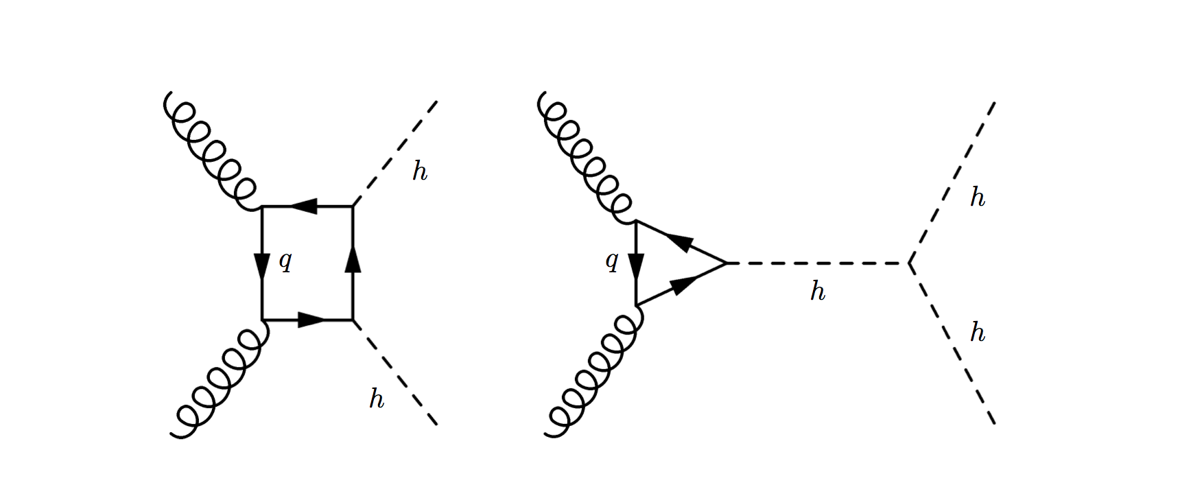
Figure 1: SM loop diagrams for Higgs pair production via gluon fusion.

Within the ADD model, the double Higgs production occurs at tree level through both $gg$ fusion and $q\bar{q}$ annihilation via $s$-channel. The representative Feynman diagrams are presented in Fig.2. As it can be seen, in the ADD model two Higgs bosons are produced at tree level via virtual gravitons exchanges. The presence of the new diagrams lead to increase the total rate of Higgs pair with respect to the SM rate. On the other hand, due to mediating spin-2 graviton one expects different kinematical properties between the Higgs pair from the SM and ADD model. These issues will be discussed more in the next sections.

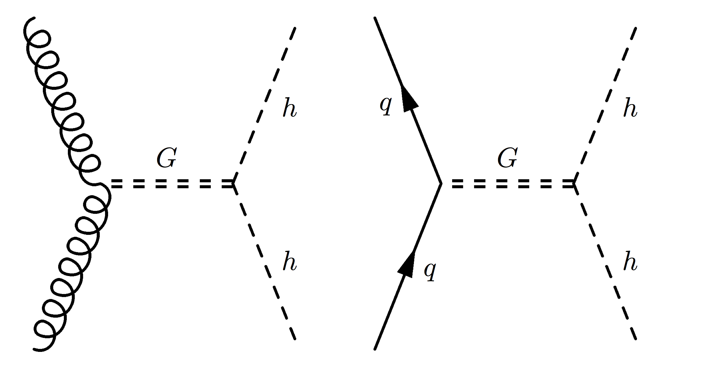
Figure 2: Tree level di-Higgs production diagrams with virtual graviton exchange in the ADD model.

In this work, Sherpa [65] event generator is used to generate the di-Higgs events and to calculate the cross sections in the ADD model. Figure 3 shows the calculated cross section of Higgs boson pair production at three different center-of-mass energies of 14, 33 and 100 TeV as a function of ADD model parameter $\Lambda_{T}$ in the GRW convention. As expected, the total production cross section of two Higgs bosons grows significantly with respect to the expectation of the SM at the three center-of-mass energies. Due to larger phase space and PDFs, the cross section increases with increasing the center-of-mass energy. Because the $gg$ and $q\bar{q}$ interactions with gravitons are suppressed by the Planck scale in $4+n_{ED}$ dimensions, the cross section is expected to decrease with increasing the ADD model scale $\Lambda_{T}$ hence the cross section goes to the SM value when $\Lambda_{T}\rightarrow\infty$.

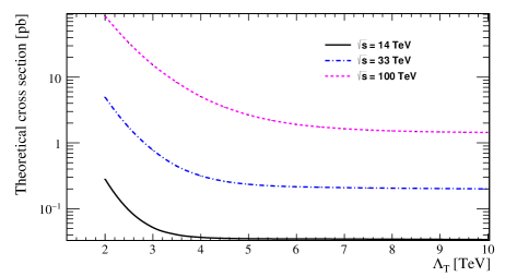
Figure 3: Cross section of pair Higgs production at three different center-of-mass energies of 14, 33 and 100 TeV as a function of $\Lambda_{T}$ in the GRW convention. It can be seen that cross sections tend to the SM ones as $\Lambda_{T}\rightarrow\infty$.

Figure 4 shows the ratio of di-Higgs cross section from $q\bar{q}$ annihilation and only $b\bar{b}$ to the total cross section versus the ADD model parameter $\Lambda_{T}$ at three collision energies of 14, 33, and 100 TeV. The contribution of the $gg$ fusion is shown in Fig.5. As expected the main contribution is coming from the $gg$ fusion with the amount of more than $60\%$ and $90\%$ at $\Lambda_{T}=2$ TeV at the center-of-mass energies of 14 and 100 TeV, respectively. With increasing the center-of-mass energy, the contribution from $gg$ fusion is increased. It is interesting to note that again with increasing the center-of-mass energy, the b-quark parton distribution function is increased which leads to larger contribution from $b\bar{b}$ annihilation at larger energies.

We close this section by mentioning that the ADD model leads to produce considerable number of Higgs boson pairs in $pp$ collisions. We will see that the increment in number of Higgs pairs in particular occurs at the large invariant mass of the two Higgs system $M_{HH}$. Such an effect will be used as a tool to search for the ADD model and constraining the model parameters at different collision energies. The details of the analysis are described in the next sections.

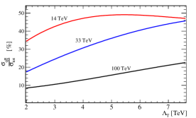
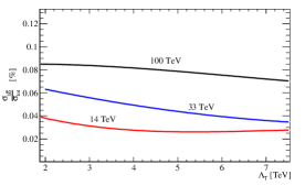
Figure 4: Ratio of partonic cross section over the total cross section for the quark anti-quark initial state.

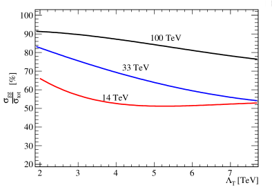
Figure 5: Ratio of partonic cross section over the total cross section for the gluon-gluon initial state.

3 Analysis Method

In this section, we explain the analysis procedure that is followed for generating and analyzing the signal of ADD model in $pp$ collisions at the LHC with $\sqrt{s}=14$ TeV and FCC. Throughout this analysis, we use a CMS-like experiment characteristics for simulating the effects of detector and similar statistical tools for obtaining the exclusion limits as the CMS experiment. We only focus on the Higgs bosons decay into $b\bar{b}$ pairs. This leads to have a final state containing four jets originating from the hadronization of b-quraks.

3.1 Event generation

The ADD signal events are generated using Sherpa version $2\_1\_1$ [65] in the GRW convention. Sherpa also performs parton showering and hadronization processes. The background with most similarity to the signal which can be interpreted as the irreducible background comes from the SM di-Higgs explained previously. The SM di-Higgs event generation is done with the MadGraph 5 [66, 67] and Pythia [68] is used to perform parton showering and hadronization. The remaining main background processes are QCD multijets, $Zb\bar{b}$ $ZZ$, $ZH$, $t\bar{t}$, single top, $W^{+}W^{-}$, $W+jets$ which are generated using Sherpa including the showering and hadronization. The contribution of multijet QCD background is difficult to reliably estimate due to large production rate. In reality, the determination of the QCD multijet contribution requires computing resources and/or employing a data-driven technique which is beyond the scope of the current work. We generate several QCD multijet samples in various bins of invariant mass of the final state partons with large amount of events in each bin.

A full and real detector effects simulation must be performed by the experimental collaboration however we use Delphes [69] as the tool to estimate the response of the detector. It considers a modeling of the CMS detector performances as explained in [70]. In this study, the effects of pileup and underlying events are not taken into account.

Finally, we should mention that the signal samples are generated with Sherpa in the GRW convention for the various values of the ADD model parameter $\Lambda_{T}$ and all simulated samples are generated for the three possible scenarios of the center-of-mass energies of proton-proton colliders, 14 TeV, 33 TeV and 100 TeV.

3.2 Analysis details

We perform the analysis of the simulated events on the stable final state particles. The selection of the events is designed in such a way to find the $HH$ events with subsequent decay of $HH\rightarrow b\bar{b}b\bar{b}$.

Before going further, one of the special characteristic of the signal events, which leads to employ particular strategies for events reconstruction and selection, is considered . In Fig.6, the normalized distribution of $\Delta R$ between two bottom quarks coming from the decay of each Higgs boson for two samples of signal with $\Lambda_{T}=3,5$ TeV and some backgrounds is shown. As it can be seen in Fig.6, signal events tend to reside at very small values of $\Delta R$ contrary to the SM backgrounds.

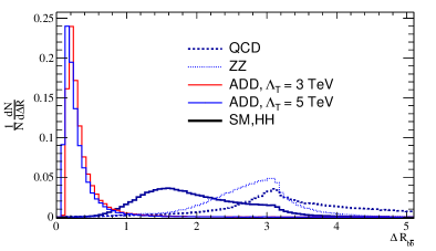
Figure 6: Normalized distribution of the $\Delta R$ between two bottom quarks coming from decay of each Higgs for the two samples of signals and the potential backgrounds.

In the events of signal with very large di-Higgs invariant mass, Higgs bosons are Lorentz-boosted particles which decay differently from the topological point of view compared to the Higgs bosons which are produced almost at rest. The angular separation of a $b\bar{b}$ pair coming from a Higgs boson can be approximated as:

$$\Delta R_{b\bar{b}}\simeq\frac{1}{\sqrt{x(1-x)}}\frac{m_{H}}{P_{T}}$$ (7)

where $P_{T}$ is the transverse momentum of the Higgs boson, $x$ and $1-x$ are the momentum fractions of the $b$ and $\bar{b}$ quarks. The larger Higgs $P_{T}$ the smaller angular separation of $b\bar{b}$ pair. Figure 7 shows two dimensional plots of $\Delta R_{b\bar{b}}$ versus the Higgs boson $P_{T}$ and the hardest $b$ quark $P_{T}$ in a Higgs boson decay for the SM process of $pp\rightarrow HH\rightarrow b\bar{b}b\bar{b}$. The plots of Figure 7 confirm that as we go to the boosted region (events with large transverse momentum of Higgs or large transverse momentum of b quark), the $\Delta R_{b\bar{b}}$ decreases. It means that the boosted Higgs bosons produce one collimated jet with substructure. This can originate from two reasons: first is that the decaying Higgs boson has an energy several times larger than the Higgs boson mass in the laboratory frame and second reason is the difference between the mass of Higgs and b quark is large.

As the di-Higgs invariant mass is an important quantity which will be used to separate ADD signal events from the backgrounds, $\Delta R_{b\bar{b}}$ is also presented versus the di-Higgs invariant mass for signal and SM di-Higgs events in Figure 8. Obviously, the ADD signal events prefer to be distributed in the large invariant mass region of the di-Higgs system which is not the case for the SM di-Higgs events. Another observation from the Figure 8 is that with increasing the di-Higgs mass of the signal events, $\Delta R_{b\bar{b}}$ decreases and falls even below 0.4. More accurately, the SM di-Higgs events are distributed at di-Higgs invariant mass smaller than 1 TeV and peak at $\Delta R=1.5$ while for the signal, di-Higgs invariant mass peak at values greater than 3 TeV and around $\Delta R=0.3$.

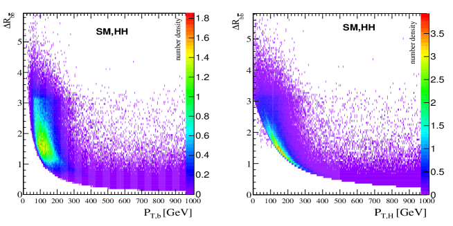
Figure 7: The transverse momentum of the hardest bottom quark and the Higgs boson transverse momentum as a function of $\Delta R$ for the SM di-Higgs events.

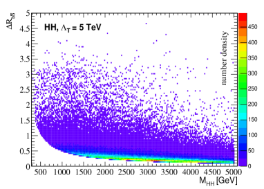
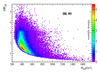
Figure 8: Invariant mass of di-Higgs as a function of the $\Delta R$ between the each b-jet pairs for the signal with $\Lambda_{T}=$ 5 TeV (left) and for the SM di-Higgs events (right).

The kinematics of the Higgs boson decay products is categorized by two types of event topologies. The first category consists of Higgs boson pairs which are produced near the threshold. In this type of events (normal events), each parton is matched to a single jet. In the second category, Higgs bosons are produced with a large Lorentz boost, resulting in collimated jets that might cluster into one jet. These events are referred as boosted events which need to be treated differently from the normal events.

3.3 Boosted jet reconstruction

As it has been mentioned previously, reconstruction of b-jets specially for the signal events due to the existence of highly boosted Higgs bosons are crucial. According to Eq.7 if the Higgs bosons have transverse momentum larger than $P_{T}>500\>GeV$ and if approximately both b-jets carry the same fractions of the Higgs boson momentum, the angular separation between two b-jets is $\Delta R<0.5$. As a consequence, common jet reconstruction which usually is done with the cone size of $\Delta R=0.4-0.5$ would not be applicable for the most of signal events. Therefore, an alternative way of fat jet algorithm is used [71] for these boosted events.

Now, the jet substructure analysis is described together with its application on our signal with four boosted b-jets in the final state. We reconstruct the fat jets using the Cambridge/Aachen (CA) jet algorithm [72, 73] assuming special jet cone size of $R=1.2$. Then to identify the boosted Higgs bosons, the procedures described in the fat jet reconstruction algorithm [71] is performed as the following. First, large radius or a fat jet $J$ is split into two sub-jets $J_{1}$ and $J_{2}$ with masses $m_{J_{1}}>m_{J_{2}}$. Then a significant mass drop of $m_{J_{1}}<\mu_{MD}m_{J}$ with $\mu=0.667$ is required. $\mu_{MD}$ is an arbitrary value that shows the degree of the mass drop. In order to avoid the inclusion of high $P_{T}$ light jets, two sub-jets have to be symmetrically split by satisfying:

$$\frac{min(P_{T,\,J_{1}}^{2},P_{T,\,J_{2}}^{2})}{m_{J}^{2}}\Delta R_{J_{1},\,J_{2}}^{2}<y_{cut}$$ (8)

where $P_{T,\,J_{1}}^{2}$and $P_{T,\,J_{2}}^{2}$ are the square of the transverse momentum of each sub-jet and $y_{cut}$ is one of the parameters of the algorithms which determines the limit of asymmetry between two sub-jets. Finally, if the criteria in the above steps are not fulfilled, we take $J=J_{1}$ and return to the first step to perform decomposition. All the above steps are followed by a filtering in which a re-clustering is performed with the radius of $R_{filt}=min(0.3,\Delta R_{J_{1},\,J_{2}}/2)$ which selects at most three hardest jets. This is a useful step to remove the contributions from pileup and underlying events [74]. In the analysis, the two hardest objects are required to be tagged as b-jets while the third one can be possible radiation of the two b quarks.

It has been shown the best values for the algorithm parameter are $\mu_{MD}=0.67$ and $y_{cut}=0.09$ [71] and the best performance for clustering when it deals with jet substructure is C/A algorithm. It is worth mentioning here that tighter value of $\mu_{MD}$ would not be useful significantly [75]. The algorithm explained above for reconstruction of the boosted objects has been implemented in the FastJet3.1.1 package [76] using that we perform the analysis to find the two Higgs bosons in the final state.

In this analysis, first the jets coming from signal or backgrounds are reconstructed with the anti-$k_{T}$ algorithm with the cone size of $R=0.5$ then if two jets with $P_{T}>250$ GeV are found in the event, the fat jet algorithm is applied. Otherwise, the event is treated as normal event.

As for the b-tagging efficiency and mis-tag rates, similar numbers as the CMS experiment are used. The data driven efficiency for the b-jet identification indicates that the efficiency is as large as $60\%$ to $80\%$ [77]. In our analysis, a b-tagging efficiency of $70\%$ for jets with transverse momentum larger than 30 GeV and in the pseudorapidity range of $|\eta|<2.5$ is assumed. Mis-tagging rates of $10\%$ and $1\%$ for the c-jets and for the light jets are considered [77].

3.4 Higgs bosons reconstruction

For reconstruction of the Higgs bosons in the final state, a $\chi^{2}$ algorithm is utilized to determine the correct assignment of b-jets to Higgs bosons candidates. It relies on the Higgs boson mass and other kinematics properties as constraints. All possible permutations for four or more b-jets are tried and the permutation with minimum $\chi^{2}$ is used to reconstruct both Higgs bosons. The $\chi^{2}$ which is run over the events containing at least four b-jets with $P_{T_{b}}>30$ GeV and $|\eta|<2.5$ is defined as:

$$\chi^{2}=(M_{ij}-M_{H})^{2}+(M_{kl}-M_{H})^{2}+\Delta R_{ij}^{2}+\Delta R_{kl}^{2}$$ (9)

where $M_{ij},\>M_{kl}$ are the invariant mass of the b-jets pairs and $M_{H}=125$ GeV. As mentioned above, the best combination of b-jet pairs is the one with minimum $\chi^{2}$ out of three possible combinations. Figure 9 shows the invariant mass of the b-jet pairs after applying the fat jet algorithm and a CMS-like detector effects. As it can be seen, the reconstructed Higgs bosons from signal have a very good resolution on the mass spectrum. For the sake of comparison, the reconstructed mass distributions of some background processes are also shown in Fig.9. Because of the efficient performance of the fat jet algorithm which leads to a better resolution on the Higgs boson mass spectrum with respect to all backgrounds, imposing cut on the invariant mass of each b-jet pairs can suppress significant amount of the backgrounds keeping signal events at a maximum level.

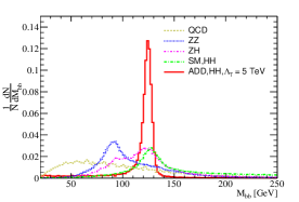
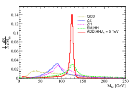
Figure 9: Normalized distributions of the reconstructed Higgs bosons for the signal and backgrounds after applying the fat jet algorithm and detector effects.

According to discussions in the first section, we expect a continuous enhancement in the rate of the signal events due to contribution of the very close $G_{kk}$ modes of gravitons. This effect manifests itself mostly in the high invariant mass region of di-Higgs events where the number of excited modes of the $G_{kk}$ are much larger. This effect has been shown previously in Fig.8, the ADD signal events have very large di-Higgs invariant mass while the SM di-Higgs events are distributed at lower invariant mass with respect to signal. Such a discriminating feature is used in the next section to set limits on the ADD signal model parameters. Figure 10 depicts the invariant mass of the two reconstructed Higgs bosons for the signal and different sources of backgrounds. This plot shows the behavior of the signal and potential backgrounds in the final state mass spectrum. In this plot, no cut except for the acceptance cuts are applied.

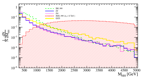
Figure 10: Invariant mass of the Higgs pair for the signal sample with the parameter of $\varLambda_{T}=5\,TeV$ and other sources of the backgrounds. distribution is normalized to the number of the each samples separately.

3.5 Event selection

To select the signal events, we require events to have exactly four b-tagged jets with $P_{T}>30$ GeV and $|\eta|<2.5$ and no isolated lepton with $P_{T}>10$ GeV. The missing transverse energy is required to be less than 10 GeV. All these requirements are denoted as cut-1. Additional cuts are applied for further backgrounds suppression. Due to good resolution on angular separation between b-jet pairs coming from each Higgs boson, we require each b-jets pair to have $\Delta R<0.6$ (cut-2). Such a tight cut reduces the contributions of non-boosted background events. A mass window cut of 100 GeV to 150 GeV is applied on the invariant mass of each reconstructed b-jets pair (cut-3) which suppresses the contribution of the backgrounds with no Higgs boson. We should mention here that triggering of the events with purely hadronic final states needs careful attention however requiring four energetic jets in the event has good enough efficiency at the LHC experiments.

Finally, we present the event yield at the center-of-mass energy of 14 TeV with 300 fb^-1 of the integrated luminosity in Table 1. In this table, the number of remaining events are presented in a signal region of $M_{HH}>1.4$ TeV for signal and main backgrounds. Table 1 explicitly shows that in the high invariant mass of di-Higgs, i.e. the signal region, the contribution of the reducible backgrounds are almost negligible and the only main source of the background comes from the SM Higgs pair production. As it can be seen and shown in [13], the combination of jet substructure techniques, b-tagging requirement, and invariant mass cuts reduces the contribution of the QCD multijet background negligible.

The cut on the di-Higgs invariant mass needs to be optimized to achieve best limits on the ADD model parameter which will be explained in the next section.

	ADD,$\Lambda_{T}=6$ TeV	SM,HH	QCD	Z$b\bar{b}$	ZZ+WW	ZH	$t\bar{t}$
Cut on $M_{HH}$				$M_{HH}>$ 1.4 TeV
cut-1	3.86	13.46	5.6e+5	1.2e+5	26.47	4.34	40.70
cut-2	3.51	1.96	13.48	31.0	0.01	0.22	0.00
cut-3	2.28	0.55	0.02	0.30	0.00	0.00	0.00

Table 1: Number of survived events of ADD signal and different backgrounds after applying sets of cut-1, cut-2, and cut-3 described in the text in the signal region of $M_{HH}>1.4$ TeV for the $\sqrt{s}=14$ TeV and with 300 $fb{}^{-1}$ of integrated luminosity of expected data from the LHC.

4 Limit calculation

In this section we present the statistical procedure that we use to obtain the expected limits on the ADD model parameter. As we mentioned formerly, the invariant mass of the Higgs pair is an effective observable that we use to set limit on the signal cross section and then translate the limit on the model parameters in the absence of any indication of the ADD model signal. A single bin counting experiment in the signal dominant region (high invariant mass region) is used to set the limits. We begin with a Poisson distribution as the probability of measuring $N$ events in the signal region:

$$P(N|\,\sigma_{ADD}\,\varepsilon\,\mathcal{L},B)=e^{-(B+\sigma_{ADD}\varepsilon\mathcal{L})}\frac{(B+\sigma_{ADD}\varepsilon\mathcal{L})^{N}}{N!}$$ (10)

where $\sigma_{ADD},\>\varepsilon,\>\mathcal{L}\>\$ and $B$ are signal cross section, signal efficiency, integrated luminosity and expected number of backgrounds. In the above equation, $\sigma_{ADD}$ is taken as a free parameter to enable us to consider different ADD signal production cross sections. To obtain the number of expected background events $B$ and the signal efficiency $\epsilon$, we rely on the Monte Carlo simulations. At confidence level of $95\%$, an upper limit on the signal rate $\sigma_{ADD}$ is obtained by integrating over the posterior probability as the following:

$$0.95=\frac{\int_{0}^{\sigma^{95\%}}P(N|\,\sigma_{ADD}\,\varepsilon\,\mathcal{L},B)d\sigma_{ADD}}{\int_{0}^{\infty}P(N|\,\sigma_{ADD}\,\varepsilon\,\mathcal{L},B)d\sigma_{ADD}}$$ (11)

In order to extract the expected limit on the ADD signal cross section, one has to solve the Eq.11 for $\sigma^{95\%}$ under the assumption of $N=B$ after inserting the proper inputs for the background expectation, signal efficiency, and the integrated luminosity.

In the first step of limit setting, we have to determine the signal dominant region. Therefore, the di-Higgs invariant mass cut which determines this region is optimized in such a way that gives the best exclusion limits on the model parameter $\varLambda_{T}$. This can be reached by minimizing the $95\%$ CL expected limit on the signal cross section. Figure 11 shows the calculated expected limit at $95\%$ CL on $\varLambda_{T}$ as a function of invariant mass cut of di-Higgs. As it can be seen in Fig.11, with increasing the cut on di-Higgs mass the exclusion limit on $\Lambda_{T}$ is maximized at the cut on di-Higgs mass of around 1.4 TeV with an integrated luminosity of 300 fb^-1. Thus, we take the mass cut of 1.4 TeV as the optimized value to introduce the signal region. It has to be mentioned that in the optimization process no systematic uncertainty is included. It is worth mentioning that the optimized cut on the di-Higgs invariant mass varies with the integrated luminosity.

We calculated the signal efficiency after applying the set of cuts described in the previous section. This efficiency has almost a flat behavior against the model parameter $\Lambda_{T}$ . The mean value of the signal efficiency is taken to calculate the limit. It is found to be equal to $17\%$. The uncertainty on the efficiency originating from statistical fluctuations and a $5\%$ uncertainty due to the fluctuation of efficiency for different $\Lambda_{T}$ are considered. An overall uncertainty of $30\%$ on the number of background events in addition to the statistical uncertainty is considered.

Figure 12 shows the expected limit at $95\%$ CL as a function of model parameter $\Lambda_{T}$ including the uncertainty bands. The theoretical cross section of ADD signal also is presented for comparison. The $95\%$ CL expected upper limit on signal cross section in the signal region is found to be $0.09$ fb for an integrated luminosity of 300 fb^-1 of data. It leads to an expected lower limit on $\Lambda_{T}$ to be 5.1 TeV. These bounds are in a reasonable agreement with the $3\sigma$ exclusion limits calculated in [57] where no object reconstruction and identification and detector effects have been considered.

Similar analyses are performed for higher center-of-mass energies of future planed proton-proton colliders with the integrated luminosities of 300 fb^-1 and 3 ab^-1. The results for expected limits on the $\Lambda_{T}$ in GRW convention and on ($n{}_{ED}$, $M{}_{S}$) in the HLZ convention are summarized in Tables 2 and 3, respectively. Moving to larger center-of-mass energy of the collisions leads to increase the lower limit on $\Lambda_{T}$. The limit is extended up to around 24 TeV at the collision energy of 100 TeV. Using more integrated luminosity of data would lead to improve the limit on the model parameter. Increasing the integrated luminosity by a factor of 10 changes the lower limit on $\Lambda_{T}$ from 5.1 TeV to 6.8 TeV at $\sqrt{s}=14$ TeV.

At the end of this section, it must be mentioned that including the other decay channels of the Higgs bosons ($\gamma\gamma,\tau^{+}\tau^{-},ZZ,WW$) would improve the limits considerably.

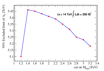
Figure 11: The $95\%$ CL expected limit on $\varLambda_{T}$ as a function of cut on the invariant mass of two reconstructed Higgs bosons.

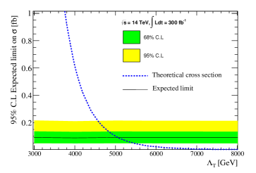
Figure 12: The $95\%$ CL expected limit on the ADD signal cross section as a function of $\Lambda_{T}$ including the uncertainty bands. The theoretical cross section of ADD model is also presented for comparison.

$\begin{array}[]{c}IL=300\;fb^{-1}\\ \text{center-of-mass~{}energy}\end{array}$	$\varLambda_{T}\>[TeV](GRW)$	$\begin{array}[]{c}M_{S}\>[TeV](HLZ)\\ n=3\;n=4\;n=5\;n=6\;n=7\end{array}\>$
$14$ TeV	5.1	$6.1\qquad 5.1\qquad 4.6\qquad 4.3\qquad 4.1$
$33$ TeV	10.5	$12.5\quad\;\;10.5\quad\;\;9.5\quad\;\;8.8\quad\;\;8.3$
$100$ TeV	23.6	$28.1\quad\;\;23.6\;\quad\;21.3\;\quad\;19.8\;\quad\;18.8$

Table 2: $95\%$ CL expected limit on the parameters of the model in both GRW and HLZ conventions for the 300 fb ^-1 of integrated luminosity of data.

$\begin{array}[]{c}IL=3\;ab^{-1}\\ \text{center-of-mass~{}energy}\end{array}$	$\varLambda_{T}\>[TeV](GRW)$	$\begin{array}[]{c}M_{S}\>[TeV](HLZ)\\ n=3\;n=4\;n=5\;n=6\;n=7\end{array}\>$
$14$ TeV	6.8	$8.1\qquad 6.8\qquad 6.1\qquad 5.7\qquad 5.4$
$33$ TeV	13.4	$16.0\quad\;\;13.4\quad\;\;12.1\quad\;\;11.3\quad\;\;10.7$
$100$ TeV	28.7	$34.1\quad\;\;28.7\;\quad\;25.9\;\quad\;24.1\;\quad\;22.8$

Table 3: $95\%$ CL expected limit on the parameters of the ADD model in both GRW and HLZ conventions for the 3 ab^-1data.

5 Di-Higgs angular distribution

An interesting feature of di-Higgs production from the large extra dimensions is the quite different behavior of the angular distribution of the final state with respect to the SM backgrounds. In general, final state particles coming from the exchange of gravitons with spin 2 should have different shape from the final state particles from the exchanges of photon, $Z$-boson or Higgs boson. On the other hand, using fat jet algorithm enabled us to have very good resolution on angular separation. Therefore, angular distribution of the Higgs boson pairs can be used as a powerful observable to distinct the ADD signal from the SM backgrounds to set limits on the model parameters.

The shape of the angular distribution of di-Higgs, which is an interesting feature of the ADD model, is shown in Fig.13. The angular distribution of the SM di-Higgs is presented for comparison. In this plot, $\theta(H_{1},H_{2})$ is the angle between the directions of the momenta of the final state Higgs bosons. The distribution of $\cos\theta(H_{1},H_{2})$ is plotted for ADD di-Higgs production from $q\bar{q}$ annihilation and $gg$ fusion separately. As it can be seen, the angular distribution of the signal events from $gg$ fusion has quite different behavior from $q\bar{q}$. The two Higgs of ADD events produced from $gg$ prefer to fly mostly perpendicular to each other while the two Higgs bosons in the ADD events from $q\bar{q}$ fusion tend to be produced at the angles of approximately $\pm\pi/4$. Detailed analytical explanations of the angular distributions of di-Higgs from the ADD model in $e^{+}e^{-}$ collisions and $\gamma\gamma$ collisions can be found in [78] and [79]. Similar explanations are valid for the hadron colliders with the initial states of $q\bar{q}$ and $gg$ are expected to be like $e^{+}e^{-}$ and $\gamma\gamma$, respectively. According to Fig.13 , the SM di-Higgs distribution is quite flat and have different shape from the ADD signal events. It is worth mentioning here that as discussed in section 1, due to larger gluon PDF at larger center-of-mass energies the contribution of $gg$ fusion in ADD signal production is increased. It has been shown in Fig. 5.

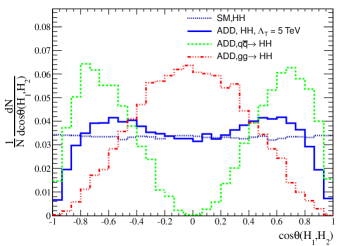
Figure 13: The distribution of $\cos\theta(H_{1},H_{2})$ for the SM di-Higgs background and the extra dimension signal at parton level.

The CMS and ATLAS collaborations [80, 81] have used a variable of $X=exp(|y_{1}-y_{2}|)$ to search for the contact interactions in di-jet events. The rapidities of the two jets are denoted by $y_{1},y_{2}$. The rapidity $y$ is defined as $\log(\frac{E+p_{z}}{E-p_{z}})$ where $E$ is the energy and $p_{z}$ is the $z$-component of the momentum of a given particle. The advantage of the rapidity difference is that it is a boost invariant quantity. Now, we use the $X=exp(|y_{H_{1}}-y_{H_{2}}|)$ distribution to probe the effects of ADD model instead of $\cos\theta(H_{1},H_{2})$.

Figure 14 shows of $X=exp(|y_{H_{1}}-y_{H_{2}}|)$ for main SM background di-Higgs and the ADD signal with $\Lambda_{T}=3$ TeV. Considering only the SM di-Higgs as the main background, we set a limit on the ADD parameter using this angular distribution. We perform the analysis with an integrated luminosity of 300 fb^-1. We define a $\chi^{2}$ over the $X$ distribution as:

$$\chi^{2}=\sum_{i=0}^{n}\frac{(N_{sig+bck}-N_{bck})^{2}}{\sqrt{\Delta_{stat}^{2}+\Delta_{syst}^{2}}}$$ (12)

where the numerator shows the square number of signals and $\Delta_{stat}$ and $\Delta_{syst}$ represent the statistical and systematical uncertainties. To calculate the $\chi^{2}$, we use the same event selections as before and we consider the events in the signal region which is determined in the previous section. Figure 15 shows the $\chi^{2}/n$ as a function of $\Lambda_{T}$, where $n$ indicates the number of degree of freedom. The dashed-line shows the value of $\chi^{2}/n$ which corresponds to the $95\%$ CL. The limit on $\Lambda_{T}$ using this observable is found to be 6.98 TeV which is higher than the value that we obtained using the invariant mass. To check the effect of systematic uncertainties, we considered $20\%$ and $40\%$ overall systematic uncertainties which are shown as dashed lines. Including $40\%$ systematic uncertainty leads to loosen the limit on $\Lambda_{T}$ around 200 GeV. A significant improvement could be achieved using the distribution of the rapidity gap of two-Higgs bosons which amounts to around 1.8 TeV with respect to the mass spectrum analysis of di-Higgs.

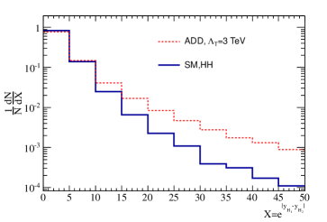
Figure 14: The normalized distribution of $\exp(y_{H_{1}}-y_{H_{2}})$ for the ADD signal events and SM di-Higgs production at parton level.

This leads to conclude that the di-Higgs final state would be a promising channel to search for the large extra dimension effects at the hadron colliders. In particular, the usage of angular distribution would lead to stringent bounds on the model parameters.

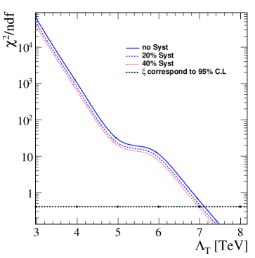
Figure 15: The $\chi^{2}/n$ as a function of $\Lambda_{T}$, where $n$ represents the number of degrees of freedom. The dashed line shows the value of $\chi^{2}/n$ which corresponds to the $95\%$ CL.

6 Summary and conclusions

Double Higgs boson production at hadron colliders provides the possibility to probe not only the Higgs self-coupling and Higgs couplings with the SM particles but also it enables us to search for the effects of new physics beyond the SM. In this paper, the double Higgs production at the LHC and future circular collider (FCC) with the center-of-mass energies of 14 TeV, 33 TeV, and 100 TeV is used to search for the effects of large extra dimensions. The analysis is only based on the most probable final state i.e. $pp\rightarrow HH\rightarrow b\bar{b}b\bar{b}$ which is of course a challenging channel due to large QCD background and triggering the events. The tail of the invariant mass of the two Higgs bosons is affected due to the virtual gravitons exchange. In addition to the di-Higgs invariant mass, the angular distributions of the final state Higgs bosons (and consequently the decay products) have a quite different behavior with respect to the SM irreducible background due to the exchange of spin 2 gravitons. We perform a comprehensive Monte-Carlo simulation analysis taking into account the main backgrounds and consider a CMS-like detector effects using the Delphes package. To reconstruct the signal candidate events efficiently and reasonable background rejection, jet substructure techniques are employed to capture the signal events which are boosted objects in the final state. Then we obtain the expected limits on the model parameters using the invariant mass and the angular properties of the final state particles. Depending on the number of extra dimensions, the effective Planck scale is limited up to 6.1, 12.5, 28.1 TeV at the proton-proton collisions with the center-of-mass energies of 14, 33, and 100 TeV, respectively. Further improvement of the analysis is possible by including other decay modes of the Higgs bosons such as $\gamma\gamma,WW,ZZ,\tau^{+}\tau^{-}$.

Acknowledgement The authors would like to thank Sherpa authors for their technical helps in ADD signal event generations.

References

- [1] G. Aad et al. [ATLAS Collaboration], Phys. Lett. B 716, 1 (2012) [arXiv:1207.7214 [hep-ex]].
- [2] S. Chatrchyan et al. [CMS Collaboration], Phys. Lett. B 716, 30 (2012) [arXiv:1207.7235 [hep-ex]].
- [3] S. Chatrchyan et al. [CMS Collaboration], JHEP 1306, 081 (2013) [arXiv:1303.4571 [hep-ex]]; G. Aad et al. [ATLAS Collaboration], Phys. Lett. B 726, 88 (2013).
- [4] G. Degrassi, S. Di Vita, J. Elias-Miro, J. R. Espinosa, G. F. Giudice, G. Isidori and A. Strumia, JHEP 1208, 098 (2012) [arXiv:1205.6497 [hep-ph]].
- [5] C. S. Chen and Y. Tang, JHEP 1204, 019 (2012) [arXiv:1202.5717 [hep-ph]].
- [6] J. Elias-Miro, J. R. Espinosa, G. F. Giudice, H. M. Lee and A. Strumia, JHEP 1206, 031 (2012) [arXiv:1203.0237 [hep-ph]].
- [7] F. R. Klinkhamer, JETP Lett. 97, 297 (2013) [arXiv:1302.1496 [hep-ph]].
- [8] E. J. Chun, S. Jung and H. M. Lee, Phys. Lett. B 725, 158 (2013) [Phys. Lett. B 730, 357 (2014)] [arXiv:1304.5815 [hep-ph]].
- [9] D. E. Ferreira de Lima, A. Papaefstathiou and M. Spannowsky, JHEP 1408, 030 (2014) [arXiv:1404.7139 [hep-ph]].
- [10] C. Csaki, J. Hubisz and S. J. Lee, Phys. Rev. D 76, 125015 (2007) [arXiv:0705.3844 [hep-ph]].
- [11] R. Barbieri, D. Buttazzo, K. Kannike, F. Sala and A. Tesi, Phys. Rev. D 87, no. 11, 115018 (2013) [arXiv:1304.3670 [hep-ph]].
- [12] J. M. No and M. Ramsey-Musolf, Phys. Rev. D 89, no. 9, 095031 (2014) [arXiv:1310.6035 [hep-ph]].
- [13] M. Gouzevitch, A. Oliveira, J. Rojo, R. Rosenfeld, G. P. Salam and V. Sanz, JHEP 1307, 148 (2013) [arXiv:1303.6636 [hep-ph]].
- [14] F. Goertz, arXiv:1504.00355 [hep-ph].
- [15] F. Goertz, A. Papaefstathiou, L. L. Yang and J. Zurita, JHEP 1504, 167 (2015) [arXiv:1410.3471 [hep-ph]].
- [16] Z. Kang, P. Ko and J. Li, arXiv:1504.04128 [hep-ph].
- [17] B. Hespel, D. Lopez-Val and E. Vryonidou, JHEP 1409, 124 (2014) [arXiv:1407.0281 [hep-ph]].
- [18] B. Bhattacherjee, A. Choudhury, Phys. Rev. D 91, 073015 (2015) [arXiv:1407.6866 [hep-ph]].
- [19] M. J. Dolan, C. Englert and M. Spannowsky, JHEP 1210, 112 (2012) [arXiv:1206.5001 [hep-ph]].
- [20] N. Arkani-Hamed, S. Dimopoulos and G. R. Dvali, Phys. Lett. B 429, 263 (1998) [hep-ph/9803315].
- [21] N. Arkani-Hamed, S. Dimopoulos and G. R. Dvali, Phys. Rev. D 59, 086004 (1999) [hep-ph/9807344].
- [22] I. Antoniadis, N. Arkani-Hamed, S. Dimopoulos and G. R. Dvali, Phys. Lett. B 436, 257 (1998) [hep-ph/9804398].
- [23] G. F. Giudice, R. Rattazzi and J. D. Wells, Nucl. Phys. B 544, 3 (1999) [hep-ph/9811291].
- [24] T. Han, J. D. Lykken and R. J. Zhang, Phys. Rev. D 59, 105006 (1999) [hep-ph/9811350].
- [25] J. L. Hewett, Phys. Rev. Lett. 82, 4765 (1999) [hep-ph/9811356].
- [26] T. Gleisberg, F. Krauss, K. T. Matchev, A. Schalicke, S. Schumann and G. Soff, JHEP 0309, 001 (2003) [hep-ph/0306182].
- [27] G. Aad et al. [ATLAS Collaboration], Phys. Rev. D 87, no. 1, 015010 (2013) [arXiv:1211.1150 [hep-ex]].
- [28] H. C. Cheng, arXiv:1003.1162 [hep-ph].
- [29] D. J. Kapner, T. S. Cook, E. G. Adelberger, J. H. Gundlach, B. R. Heckel, C. D. Hoyle and H. E. Swanson, Phys. Rev. Lett. 98, 021101 (2007) [hep-ph/0611184].
- [30] C. Adloff et al. [H1 Collaboration], Phys. Lett. B 479, 358 (2000) [hep-ex/0003002].
- [31] S. Chekanov et al. [ZEUS Collaboration], Phys. Lett. B 591, 23 (2004) [hep-ex/0401009].
- [32] P. Abreu et al. [DELPHI Collaboration], Phys. Lett. B 491, 67 (2000) [hep-ex/0103005].
- [33] G. Abbiendi et al. [OPAL Collaboration], Eur. Phys. J. C 17, 553 (2000) [hep-ex/0007016].
- [34] P. Abreu et al. [DELPHI Collaboration], Phys. Lett. B 485, 45 (2000) [hep-ex/0103025].
- [35] G. Abbiendi et al. [OPAL Collaboration], Eur. Phys. J. C 26, 331 (2003) [hep-ex/0210016].
- [36] V. M. Abazov et al. [D0 Collaboration], Phys. Rev. Lett. 95, 161602 (2005) [hep-ex/0506063].
- [37] V. M. Abazov et al. [D0 Collaboration], Phys. Rev. Lett. 102, 051601 (2009) [arXiv:0809.2813 [hep-ex]].
- [38] S. Chatrchyan et al. [CMS Collaboration], JHEP 1105, 085 (2011) [arXiv:1103.4279 [hep-ex]].
- [39] CS. Chatrchyan et al. [CMS Collaboration], Phys. Rev. Lett. 108, 111801 (2012) [arXiv:1112.0688 [hep-ex]].
- [40] G. Aad et al. [ATLAS Collaboration], Phys. Lett. B 710 (2012) 538 [arXiv:1112.2194 [hep-ex]].
- [41] G. Aad et al. [ATLAS Collaboration], Eur. Phys. J. C 74 (2014) 12, 3134 [arXiv:1407.2410 [hep-ex]].
- [42] V. Khachatryan et al. [CMS Collaboration], JHEP 1504, 025 (2015) [arXiv:1412.6302 [hep-ex]].
- [43] V. Khachatryan et al. [CMS Collaboration], Eur. Phys. J. C 75, no. 5, 235 (2015) [arXiv:1408.3583 [hep-ex]].
- [44] G. Aad et al. [ATLAS Collaboration], Eur. Phys. J. C 74, no. 12, 3134 (2014) [arXiv:1407.2410 [hep-ex]].
- [45] S. B. Giddings and S. Thomas, Phys. Rev. D 65, 056010 (2002).
- [46] S. Dimopoulos and G. Landsberg, Phys. Rev. Lett. 87, 161602 (2001).
- [47] V. Barger, T. Han, C. Kao, and R.J. Zhang, Phys. Lett. B 461 (1999) 34.
- [48] L. J. Hall, D. Smith, Phys.Rev.D 60 (1999) 085008.
- [49] G. Dvali and G. Gabadadze, Phys. Lett. B 460 (1999) 47.
- [50] J. Khoury, B. A. Ovrut, P. J. Steinhardt, N. Turok, Phys. Rev. D 64 (2001) 123522.
- [51] M. Masip and A. Pomarol, Phys. Rev. D 60, 096005 (1999) [hep-ph/9902467].
- [52] T. G. Rizzo and J. D. Wells, Phys. Rev. D 61, 016007 (2000) [hep-ph/9906234].
- [53] G. R. Dvali and A. Y. Smirnov, Nucl. Phys. B 563, 63 (1999) [hep-ph/9904211].
- [54] R. Barbieri, P. Creminelli and A. Strumia, Nucl. Phys. B 585, 28 (2000) [hep-ph/0002199].
- [55] A. Chopovsky, M. Eingorn and A. Zhuk, Phys. Rev. D 85, 064028 (2012) [arXiv:1107.3388 [gr-qc], arXiv:1107.3388 [gr-qc]].
- [56] M. Eingorn and A. Zhuk, Class. Quant. Grav. 27, 205014 (2010) [arXiv:1003.5690 [gr-qc]].
- [57] H. Sun, Y. J. Zhou and H. Chen, Eur. Phys. J. C 72, 2011 (2012) [arXiv:1211.5197 [hep-ph]].
- [58] X. G. He, Phys. Rev. D 60, 115017 (1999) [hep-ph/9905295].
- [59] N. Delerue, K. Fujii and N. Okada, Phys. Rev. D 70, 091701 (2004) [hep-ex/0403029].
- [60] C. S. Kim, K. Y. Lee and J. H. Song, Phys. Rev. D 64, 015009 (2001) [hep-ph/0009231].
- [61] E. W. N. Glover and J. J. van der Bij, Nucl. Phys. B 309, 282 (1988).
- [62] O. J. P. Eboli, G. C. Marques, S. F. Novaes and A. A. Natale, Phys. Lett. B 197, 269 (1987).
- [63] J. Baglio, A. Djouadi, R. Gröber, M. M. Mühlleitner, J. Quevillon and M. Spira, JHEP 1304 (2013) 151 [arXiv:1212.5581 [hep-ph]].
- [64] H. L. Lai, J. Huston, Z. Li, P. Nadolsky, J. Pumplin, D. Stump and C.-P. Yuan, Phys. Rev. D 82, 054021 (2010) [arXiv:1004.4624 [hep-ph]].
- [65] T. Gleisberg, S. Hoeche, F. Krauss, M. Schonherr, S. Schumann, F. Siegert and J. Winter, JHEP 0902 (2009) 007 [arXiv:0811.4622 [hep-ph]].
- [66] J. Alwall, M. Herquet, F. Maltoni, O. Mattelaer and T. Stelzer, JHEP 1106, 128 (2011) [arXiv:1106.0522 [hep-ph]].
- [67] R. Frederix, S. Frixione, V. Hirschi, F. Maltoni, O. Mattelaer, P. Torrielli, E. Vryonidou and M. Zaro, Phys. Lett. B 732, 142 (2014) [arXiv:1401.7340 [hep-ph]].
- [68] T. Sjostrand, S. Mrenna and P. Z. Skands, JHEP 0605, 026 (2006) [hep-ph/0603175].
- [69] S. Ovyn, X. Rouby and V. Lemaitre, arXiv:0903.2225 [hep-ph].
- [70] G. L. Bayatian et al. [CMS Collaboration], J. Phys. G 34, 995 (2007).
- [71] J. M. Butterworth, A. R. Davison, M. Rubin and G. P. Salam, Phys. Rev. Lett. 100, 242001 (2008) [arXiv:0802.2470 [hep-ph]].
- [72] Y. L. Dokshitzer, G. D. Leder, S. Moretti and B. R. Webber, JHEP 9708, 001 (1997) [hep-ph/9707323].
- [73] M. Wobisch and T. Wengler, In *Hamburg 1998/1999, Monte Carlo generators for HERA physics* 270-279 [hep-ph/9907280].
- [74] A. Altheimer, S. Arora, L. Asquith, G. Brooijmans, J. Butterworth, M. Campanelli, B. Chapleau and A. E. Cholakian et al., J. Phys. G 39, 063001 (2012) [arXiv:1201.0008 [hep-ph]].
- [75] J. R. Walsh and S. Zuberi, arXiv:1110.5333 [hep-ph].
- [76] M. Cacciari, G. P. Salam and G. Soyez, Eur. Phys. J. C 72, 1896 (2012) [arXiv:1111.6097 [hep-ph]].
- [77] S. Chatrchyan et al. [CMS Collaboration], JINST 8, P04013 (2013) [arXiv:1211.4462 [hep-ex]].
- [78] N. Delerue, K. Fujii and N. Okada, Phys. Rev. D 70, 091701 (2004) [hep-ex/0403029].
- [79] X. G. He, Phys. Rev. D 60, 115017 (1999) [hep-ph/9905295].
- [80] G. Aad et al. [ATLAS Collaboration], Phys. Lett. B 694, 327 (2011) [arXiv:1009.5069 [hep-ex]].
- [81] V. Khachatryan et al. [CMS Collaboration], Phys. Rev. Lett. 105, 211801 (2010) [arXiv:1010.0203 [hep-ex]].