Classical Liquids in Fractal Dimension

Abstract

We introduce fractal liquids by generalizing classical liquids of integer dimensions $d=1,2,3$ to a non-integer dimension $d_{l}$. The particles composing the liquid are fractal objects and their configuration space is also fractal, with the same dimension. Realizations of our generic model system include microphase separated binary liquids in porous media, and highly branched liquid droplets confined to a fractal polymer backbone in a gel. Here we study the thermodynamics and pair correlations of fractal liquids by computer simulation and semi-analytical statistical mechanics. Our results are based on a model where fractal hard spheres move on a near-critical percolating lattice cluster. The predictions of the fractal Percus-Yevick liquid integral equation compare well with our simulation results.

The liquid state, an intermediate between gas and solid, exhibits short-ranged particle pair correlations in isotropic shells around a tagged particle Hansen_McDonald2006 . While the shell structure is lost for gases, solids exhibit long-ranged correlations and anisotropy. Particle correlations are accessible by experiments Kegel2000 ; Royall2008 and contain valuable information about the particle interactions. A fundamental task in theory and computer simulation of the liquid state is to predict particle correlations for given interactions. In this respect, one particularly successful approach is liquid integral equation theory Hansen_McDonald2006 ; Caccamo1996 .

Molecular and colloidal liquids can be restricted to one or two spatial dimensions Alba-Simionesco2006 ; Schoen2007 by confining them on substrates Deutschlaender2013 , at interfaces Zahn2000 , between plates Neser1997 ; Steward2014 , in channeled matrices Hahn1996 or optical landscapes Wei2000 . The thermodynamic properties change accordingly Franosch2012 and the systems are called one-dimensional (1D) or two-dimensional (2D) liquids. While these classical examples of confinement involve integer-dimensional configuration spaces, there are also cases where liquids are confined in porous media Kurzidim2009 ; Kim2011a ; Skinner2013 ; torquato2002random , or along quenched polymer coils Barrat_Hansen2003 , and where the configuration space exhibits non-integer (fractal) dimension at suitable length scales. Much work has been devoted to understanding the limiting cases of low and high density, namely the motion of a single particle on a fractal Metzler2000 ; benAvraham_Havlin2000 ; Seeger2009 ; Muelken2011 ; Hofling2013 and the structure of a fractal aggregate itself, corresponding to an arrested high-density particulate system Wong1992 ; Meakin1999 ; Sorensen2001 ; Zhao2005 ; Poon1995 . In all these situations, particles interact in the embedding integer-dimensional space and interaction energies depend on Euclidean particle distance.

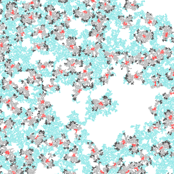
Fig. 1: (Color online) Snapshot of a Monte Carlo simulation where $300$ fractal particles are located on a percolating cluster shown in blue. The dimension of each particle and of the cluster is $d_{l}=1.67659$, and the chemical distance diameter of each particle is $\sigma=300a$ (c.f., Fig. 2). Red, black and gray pixels are occupied by particles. Red: Particle center regions (chemical distance to a particle center is less than $0.1\sigma$). Black: Particle rim regions (chemical distance to a particle center is more than $0.4\sigma$ and less than $0.5\sigma$). Gray: Regions between particle centers and rims. Every pixel in the figure corresponds to one vertex in the simulation. One quarter of the whole simulation box is shown, containing here $72$ particle centers.

In this letter, we break new ground by considering fractal particles in a fractal configuration space, both of the same non-integer dimension. An alternative model in which the particle dimension differs from the configuration-space dimension is briefly mentioned near the end of the letter. Figure  1 is a snapshot from one of our Monte Carlo (MC) simulations. The interaction between two particles is not described by a pair potential in Euclidean space, but instead inherits fractal character from the particles and their configuration space. Unifying the two complementary fields of classical liquid state theory and fractal structures, we refer to the explored, dense disordered phases as ’fractal liquids’. As opposed to continuum-mechanical descriptions of fluid flow on fractals Onda1996 ; Moreles2013 or liquids forming fractal stream networks Tarboton1988 ; Tomassone1996 , here we calculate the correlations of individual fractal particulates that constitute a liquid. We develop basic concepts for statistical mechanics of fractal liquids by presenting MC simulations along with an accurate semi-analytical fractal liquid integral equation approach. Our model system is a fractal hard sphere liquid, the analogue of the simplest generic model liquid in integer dimensions. In the present proof of principle, we restrict our studies to the liquid state. Determination of the full phase diagram of fractal particles in fractal space is a task that should be tackled in future work. In particular, it will be interesting to study whether or not symmetry breaking and crystallization occur in fractal spaces.

Fractal liquids are not only interesting from a theoretical perspective, but are also found in nature. Porous media filled with phase-separated binary liquids such as water and oil appear in natural oil or gas reservoirs, and are produced during hydraulic fracturing in oil drilling. If the oil droplets exceed the porosity length scale in size, they adapt to the fractal shape of the void space. Such droplets constitute fractal ’particles’ in a fractal configuration space set by the porous medium. While the individual water and oil molecules are confined to the void space, it is important to note that the mesoscopic water or oil droplets are not necessarily confined: If the size of the void space greatly exceeds the droplet size, then the droplets move in a (quasi) unbounded configuration space of their own non-integer dimension. Here we study the collective bulk-phase thermodynamics of such droplets, which are the fractal liquid constituents. Other possible model systems include different mesoscopic ’particles’, such as floppy slime molds Baumgarten2014 or droplets confined to fractal polymer aggregates in a gel.

To model a fractal liquid we first need a fractal-dimensional configuration space with a suitable distance measure. A viable choice is a large set of vertices on a discrete lattice for a fractal lattice liquid simulation. From a regular square lattice with a number $W$ of vertices and periodic boundary conditions in embedding 2D Euclidean space, we randomly remove vertices until $V$ vertices are left. According to percolation theory Stauffer_Aharony1994 ; benAvraham_Havlin2000 , in the limit $W\to\infty$ there is a critical percolation threshold $p_{c}=V/W$ at which a fractal-dimensional percolating cluster extends to infinite length scales. For the square lattice, a threshold of $p_{c}=0.5927\ldots$ has been reported Newman2000 .

Throughout this work, all distances $l$ between vertices are evaluated as shortest distances on the percolating cluster, using our own implementation of what is essentially equal to Dijkstra’s algorithm Dijkstra1959 . The distance between two vertices is $l=a$ if and only if these vertices are connected by a bond in one of the two Cartesian directions of the embedding space. Illustrated in Fig. 2, this distance measure is commonly referred to as ’chemical distance’ and the corresponding non Euclidean metric is known as the ’taxicab metric’.

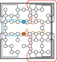
Fig. 2: (Color online) Lattice schematic. From an $8\times 8$ square lattice with periodic boundaries, $17$ vertices have been removed. Circles are the remaining vertices and black lines are the bonds of length $a$. The chemical distance between the orange and the blue filled circle is $l=8a$ along any of the three paths indicated by red, blue and orange arrows. The corresponding Euclidean distance is $r=2a$.

The lattice in Fig. 2 features the essential properties of the lattices in our simulations, except of their much larger size of $W=3000\times 3000$, $V=5~{}355~{}000$. The ratio $V/W=0.595$ is $0.4\%$ larger than $p_{c}$, which ensures the presence of a percolating cluster in the finite system. We retain only those vertices that belong to the percolating cluster. All other vertices, either in smaller clusters or isolated, are deleted. An average count of $3\times 10^{6}$ connected vertices remains. As shown in Fig. 3, the average number $P(l)$ of vertices with chemical distance $l$ from a tagged vertex grows as a non-integer power of $l$.

The so-called ’spreading dimension’ $d_{l}=1.67659\ldots$ of the percolating cluster is the relevant dimension here. It has been determined by MC simulations Zhou2012 which agree with our result $P(l)\propto l^{d_{l}-1}$. Note that $d_{l}$ differs from the more commonly reported fractal cluster dimension $d_{f}=91/48$ benAvraham_Havlin2000 ; Stauffer_Aharony1994 ; Zhou2012 , because chemical distance scales as a non-integer power of Euclidean distance.

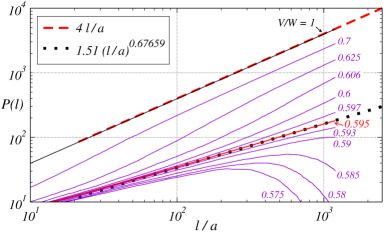
Fig. 3: (Color online) Fractal clustersize scaling. Solid curves indicate average numbers, $P(l)$, of vertices with chemical distance $l$ from a tagged vertex, in the largest cluster remaining from a lattice of initially $W=3000\times 3000$ vertices. Results are for various numbers $W-V$ of removed vertices, with ratios $V/W$ as indicated. Upper dashed line: $P(l)=4~{}l/a$, corresponding to a 2D lattice. Lower dotted line: $P(l)=1.51~{}{(l/a)}^{0.67659}$, corresponding to a $1.67659$-dimensional lattice. Our simulations are for $V/W=0.595$.

We define a fractal particle as the set of vertices that are within a distance $l\leq\sigma/2$ from a center vertex. There is exactly one center vertex per particle and we refer to $\sigma$ as the particle diameter. Every particle occupies at least one vertex pair with distance $l=\sigma$ at all times. Particles obey a no-overlap constraint, prohibiting configurations in which any two particle centers have a distance of $l\leq\sigma$. We choose $\sigma=300a$, with the consequence that the particles themselves are fractal objects (c.f. Fig. 3). As the snapshot in Fig. 1 shows, the particles are highly anisotropic in the embedding 2D space. However, in fractal space and taxicab metric, the particles and their no-overlap interactions are perfectly isotropic. In spite of their polymorphy in embedding space, all particles are indistinguishable for the purpose of our simulation. Hence the particles are fractal-dimensional analogues of monodisperse hard spheres, and one may refer to the simulated system as the $1.67659$-dimensional hard sphere liquid.

We probe the thermodynamic equilibrium state by MC simulation. Particles are moved one at a time, and every move proceeds as follows: After deleting a random particle, we pick a random vertex $v_{1}$ globally from the cluster, which is a candidate to become a vertex at the rim of the displaced particle. We then pick a random vertex $v_{2}$ at distance $l=\sigma$ from $v_{1}$, and a random vertex $v_{3}$ at distance $l=\sigma/2$ from both $v_{1}$ and $v_{2}$. Vertex $v_{3}$ is the candidate to become the displaced particle’s center vertex. If there is a center vertex of another particle at distance $l\leq\sigma$ from $v_{3}$, then the move is rejected and the original particle restored. Otherwise, the move is accepted.

The simulation starts with a random configuration of potentially overlapping particles with diameter $\sigma=10a$. In the initial simulation stage $\sigma$ is gradually inflated to $300a$, which facilitates finding a dense configuration without overlaps. After the initial inflation and equilibration the production stage is entered, and the average number $N(l)$ of particles with center-to-center distance $l$ is recorded. Binning the function $N(l)$ with a bin width of $5a$ reduces scatter in the data. Inside a fractal control volume, the fractal packing fraction $\phi$ is measured as the average number ratio of vertices occupied by particles to the total number of contained vertices. The control volume is a set of vertices with distance $l\leq 1500a$ from a center vertex. It is randomly moved during the simulation and contains at least one vertex pair with distance $l=3000a$ at all times. We compute the chemical distance distribution function

$$g(l)=c~{}\times~{}N(l)~{}\times~{}{(a/l)}^{d_{l}-1},$$ (1)

with the $l$-independent factor $c$ chosen such that $g(l)\to 1$ for large $l$. Function $g(l)$ is the analogue of the radial distribution function $g(r)$ of isotropic liquids in integer dimensions Hansen_McDonald2006 . Our simulations require long runtimes due to the numerically expensive distances calculations. The fractal cluster’s ramified structure severely complicates any performance improvement, except for parallel execution of statistically independent runs and subsequent averaging.

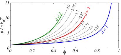
Fig. 4: (Color online) Equations of state for hard spheres in dimensions from $d=1$ to $d=3$. Thick blue curve: Exact (Tonks gas / PY) result for $d=1$. Thick red curve: Kolafa-Rottner Kolafa2006 virial series with 15 coefficients for $d=2$. Thick green curve: Carnahan-Starling equation of state for $d=3$. Thin black curves are the PY virial pressure results for dimensions as indicated.

The Ornstein-Zernike equation for a homogeneous and isotropic liquid in integer-dimensional Euclidean space reads

$$g(r)=1+c(r)+n\int d^{d}\bm{r}^{\prime}[g(r^{\prime})-1]~{}c(|\bm{r}-\bm{r}^{\prime}|),$$ (2)

where $n$ is the particle number density, $c(r)$ is the direct correlation function Hansen_McDonald2006 , $\bm{r}$ is a $d$-dimensional vector with Euclidean norm $r=|\bm{r}|$, and $d^{d}\bm{r}^{\prime}$ is an infinitesimal volume element at position $\bm{r}^{\prime}$. In conjunction with the no overlap constraint $g(r\leq\sigma)=0$ and the approximation $c(r>\sigma)=0$, Eq. (2) constitutes the Percus-Yevick (PY) integral equation for $d$-dimensional hard spheres Percus1958 , which can be systematically derived by functional Taylor expansion Hansen_McDonald2006 .

We solve the PY equation by means of a spectral solver Heinen2014 . Our numerically efficient algorithm for the convolution-type Eq. (2) is based on the Hankel transform pair

$$\tilde{f}(q) = \frac{{(2\pi)}^{d/2}}{q^{d/2-1}}\int\limits_{0}^{\infty}dr~{}r^{d/2}f(r)J_{d/2-1}(qr),$$ (3)

$${f}(r) = \frac{r^{1-d/2}}{{(2\pi)}^{d/2}}\int\limits_{0}^{\infty}dq~{}q^{d/2}\tilde{f}(q)J_{d/2-1}(qr),$$ (4)

for a $d$-dimensional isotropic function $f$, sampled on a logarithmic grid Talman1978 ; Rossky1980 ; Hamilton2000 . In Eqs. (3) and (4), $J_{d/2-1}(x)$ is the Bessel function of the first kind and order $d/2-1$. Since $J_{d/2-1}(x)$ is analytic with respect to both $x$ and $d$, the solution can be carried out formally also for non-integer dimensions. Resulting pair-correlations and thermodynamic properties represent the analytic continuations of standard PY theory with respect to the dimension.

The capability of liquid integral equations to predict thermodynamic properties in arbitrary dimension is exhibited in Fig. 4, featuring equations of state for hard spheres in various dimensions from $d=1$ to $d=3$. Thin black curves in Fig. 4 represent the $d$-dimensional hard sphere reduced virial pressure $p/nk_{B}T=1+2^{(d-1)}\phi g(r=\sigma^{+})$ with Boltzmann constant $k_{B}$, absolute temperature $T$, packing fraction $\phi=2\pi^{d/2}(\sigma/2)^{d}n/d\Gamma(d/2)$, and $g(r)$ calculated in the PY scheme. Thick curves in Fig. 4 are exact or nearly exact reference solutions for $d=1,2$ and $3$. For $d=1$, the PY result reduces to the exact (Tonks gas) solution $p/nk_{B}T=1/(1-\phi)$. The good agreement of the PY-scheme with the numerically accurate result from Ref. Kolafa2006 for $d=2$ verifies the fidelity of the PY scheme for $1\leq d\leq 2$. Comparison to the Carnahan-Starling equation of state $p/nk_{B}T\approx(1+\phi+\phi^{2}-\phi^{3})/(1-\phi)^{3}$ for $d=3$ reveals a decreasing PY-scheme accuracy for higher dimensions at large values of $\phi$.

Figure 5 shows the functions $g(l)$ extracted from our simulations with $300$ and $150$ particles. Also shown are the PY-scheme solutions $g(r)$ for $d=1$, $d=d_{l}=1.67659$ and $d=2$ and for $\phi=0.487$ and $0.266$. With the values of $\phi$ determined in the simulation, the PY scheme is free of adjustable parameters. The PY-scheme solutions for $d=d_{l}=1.67659$ agree best with the simulation data, which is most clearly seen for the higher density liquid (Fig. 5, upper panel). Note that the chemical distance range in Fig. 5 is the same as in Fig. 3, where the fractal-dimensional cluster scaling is validated.

We have also simulated 2D hard disks with center-of-mass positions confined to a fractal configuration space of dimension $d<2$ (results not shown). This constitutes an alternative fractal liquid model system, where particle dimension differs from configuration space dimension. Pair correlations in such liquids differ distinctly from the predictions of the fractal-dimensional PY scheme. This can be rationalized by noting that the PY-scheme equations are based on one and only one measure of distance, which is incapable of describing both a fractal-space correlation and an embedding-space interaction.

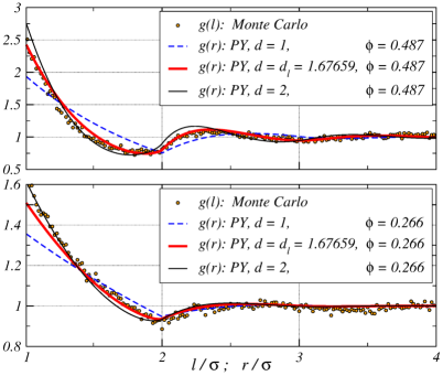
Fig. 5: (Color online) Symbols: Chemical distance distribution functions $g(l)$ from our MC simulations. Curves: PY solutions $g(r)$, for dimensions and (fractal) packing fractions as indicated. Top and bottom panels are for $300$ and $150$ simulated particles, respectively.

In conclusion, we have simulated a fractal liquid in thermodynamic equilibrium and demonstrated that the measured particle correlations are well predicted by a fractal liquid integral equation. Our approach may be easily applied to other configuration spaces with different fractal dimension. Particle interactions beyond the simple no overlap constraint should soon be studied, including short-ranged attraction which should result in liquid-vapor demixing, and also long-ranged repulsion. We have reported here on a monodisperse model system, but interaction-polydispersity is already implemented in the liquid integral equation solver for arbitrary dimension.

Fractal liquids lead the way for a plethora of new fundamental research. At present it is unclear which types of thermodynamic phases exist in fractal dimensions and phase diagrams await to be outlined. Field theories like density functional theory could be generalized to non-integer dimension. Mode coupling theory for the kinetic glass transition of three-dimensional liquids in porous media Krakoviack2005 and in arbitrary dimensions Ikeda2010 ; Charbonneau2011 relies on static structure input, which can be calculated using fractal liquid integral equations. Future studies should cover time-resolved dynamics of fractal liquids in and out of equilibrium. Transport coefficients of fractal liquids may be studied, requiring an account for fractal hydrodynamics. A promising application for fractal liquid theory is the prediction of thermodynamic properties of microphase separated liquids in porous media as encountered in natural oil and gas reservoirs.

- (1) J.-P. Hansen and I. R. McDonald. Theory of Simple Liquids. Elsevier Academic Press, Amsterdam, 3rd edition, 2006.
- (2) W.K. Kegel and A. van Blaaderen. Science, 287:290–293, 2000.
- (3) C. P. Royall, S. R. Williams, T. Ohtsuka, and H. Tanaka. Nature Materials, 7:556–561, 2008.
- (4) C. Caccamo. Phys. Rep., 274:1–105, 1996.
- (5) C. Alba-Simionesco, B. Coasne, G. Dosseh, G. Dudziak, K. E. Gubbins, R. Radhakrishnan, and M. Sliwinska-Bartkowiak. J. Phys.-Condes. Matter, 18:R15–R68, 2006.
- (6) M. Schoen and S. Klapp. Nanoconfined fluids: Soft matter between two and three dimensions. Reviews in computational chemistry, 24:1–509, 2007.
- (7) S. Deutschländer, T. Horn, H. Löwen, G. Maret, and P. Keim. Phys. Rev. Lett., 111:098301, 2013.
- (8) K. Zahn and G. Maret. Phys. Rev. Lett., 85:3656–3659, 2000.
- (9) S. Neser, C. Bechinger, P. Leiderer, and T. Palberg. Phys. Rev. Lett., 79:2348–2351, 1997.
- (10) M. C. Stewart and R. Evans. J. Chem. Phys., 140:134704, 2014.
- (11) K. Hahn, J. Kärger, and V. Kukla. Phys. Rev. Lett., 76:2762–2765, 1996.
- (12) Q.-H. Wei, C. Bechinger, and P. Leiderer. Science, 287:625–627, 2000.
- (13) T. Franosch, S. Lang, and R. Schilling. Phys. Rev. Lett., 109:240601, 2012.
- (14) J. Kurzidim, D. Coslovich, and G. Kahl. Phys. Rev. Lett., 103:138303, 2009.
- (15) K. Kim, K. Miyazaki, and S. Saito. J. Phys. Condens. Matter, 23:234123, 2011.
- (16) T. O. E. Skinner, S. K. Schnyder, D. G. A. L. Aarts, J. Horbach, and R. P. A. Dullens. Phys. Rev. Lett., 111:128301, 2013.
- (17) S. Torquato. Random heterogeneous materials: microstructure and macroscopic properties, volume 16. Springer Science & Business Media, 2002.
- (18) J.-L. Barrat and J.-P. Hansen. Basic Concepts for Simple and Complex Liquids. Cambridge University Press, 2003.
- (19) R. Metzler and J. Klafter. Phys. Rep., 339:1–77, 2000.
- (20) D. ben Avraham and S. Havlin. Diffusion and Reactions in Fractals and Disordered Systems. Cambridge University Press, Cambridge CB2 2RU, UK, 2000.
- (21) S. Seeger, K. H. Hoffmann, and C. Essex. J. Phys. A-Math. Theor., 42:225002, 2009.
- (22) O. Mülken and A. Blumen. Phys. Rep., 502:37–87, 2011.
- (23) F. Höfling and T. Franosch. Rep. Prog. Phys., 76(4):046602, 2013.
- (24) P.-z. Wong and Q.-z. Cao. Phys. Rev. B, 45:7627–7632, 1992.
- (25) P. Meakin. J. Sol-Gel Sci. Technol., 15:97–117, 1999.
- (26) C. M. Sorensen. Aerosol Sci. Technol., 35:648–687, 2001.
- (27) H. Zhao. Chem. Eng. Commun., 192:145–154, 2005.
- (28) W. C. K Poon, A. D. Pirie, and P. N. Pusey. Faraday Discuss., 101:65–76, 1995.
- (29) T. Onda, S. Shibuichi, N. Satoh, and K. Tsujii. Langmuir, 12:2125–2127, 1996.
- (30) M. A. Moreles, J. Peña, S. Botello, and R. Iturriaga. Transp. Porous Media, 99:161–174, 2013.
- (31) D. G. Tarboton, R. L. Bras, I. Rodriguez-Iturbe. Water Resour. Res., 24:1317-1322, 1988.
- (32) M. S. Tomassone, J. Krim. Phys. Rev. E, 54:6511-6515, 1996.
- (33) W. Baumgarten and M. J. B. Hauser. EPL, 108:50010, 2014.
- (34) D. Stauffer and A. Aharony. Introduction to Percolation Theory. Taylor & Francis Inc., Bristol, PA, revised 2nd edition, 1994.
- (35) M. E. J. Newman and R. M. Ziff. Phys. Rev. Lett., 85:4104–4107, 2000.
- (36) E. W. Dijkstra. Numerische Mathematik, 1:269–271, 1959.
- (37) Z. Zhou, J. Yang, Y. Deng and R. M. Ziff. Phys. Rev. E, 86:061101, 2012.
- (38) J. Kolafa and M. Rottner. Mol. Phys., 104:3435–3441, 2006.
- (39) J. K. Percus and G. J. Yevick. Phys. Rev., 110:1–13, 1958.
- (40) M. Heinen, E. Allahyarov, and H. Löwen. J. Comput. Chem., 35:275–289, 2014.
- (41) J. D. Talman. J. Comput. Phys., 29:35–48, 1978.
- (42) P. J. Rossky and H. L. Friedman. J. Chem. Phys., 72:5694–5700, 1980.
- (43) A. J. S. Hamilton. Mon. Not. R. Astron. Soc., 312:257, 2000.
- (44) V. Krakoviack. Phys. Rev. Lett., 94:065703, 2005.
- (45) A. Ikeda and K. Miyazaki. Phys. Rev. Lett., 104:255704, 2010.
- (46) P. Charbonneau, A. Ikeda, G. Parisi, and F. Zamponi. Phys. Rev. Lett., 107:185702, 2011.