Perfect plasticity with damage and healing at small strains, its modelling, analysis, and computer implementation

Abstract

The quasistatic, Prandtl-Reuss perfect plasticity at small strains is combined with a gradient, reversible (i.e. admitting healing) damage which influences both the elastic moduli and the yield stress. Existence of weak solutions of the resulted system of variational inequalities is proved by a suitable fractional-step discretisation in time with guaranteed numericalstability and convergence. After finite-element approximation, this scheme is computationally implemented and illustrative 2-dimensional simulations are performed. The model allows e.g. for application in geophysical modelling of re-occurring rupture of lithospheric faults. Resulted incremental problems are solved in MATLAB by quasi-Newton method to resolve elastoplasticity component of the solution while damage component is obtained by solution of a quadratic programming problem.

1 Introduction

There is a vast amount of literature about plasticity and about damage separately, both in mathematics and in civil or mechanical engineering. Much less literature addresses various combination of plasticity and damage, cf. e.g. [2, 3, 9, 10, 25, 27, 51]. In engineering, this is usually called ductile damage, cf. e.g. [18, 28, 29, 30, 35]. Also a lot of geophysical models combine reversible damage (called rather ageing) with some sort of plasticity (often modelled as not entirely independent of damage, however), cf. e.g. [32].

The goal of this article is to devise a model that would allow for
$\bullet$ modelling of thin plastic shear bands surrounded by wider damage zones (as typically occurs in geophysical modeling of lithospheric faults with very narrow core) with possible healing of damage (as considered in geophysical modeling to allow re-occurring damaging), and simultaneously $\bullet$ rigorous proof of existence of weak solutions of the resulted system of variational inequalities proved by a suitable fractional-step discretisation in time with guaranteed numerical stability and convergence, and $\bullet$ efficient numerical implementation of the time-discrete model. We depart from the standard linearized, associative, rate-independent plasticity at small strain as presented e.g. in [24]. Simultaneously, we use also a rather standard scalar (i.e. isotropic) damage as introduced by L.M. Kachanov in late 60ieth and presented e.g. in [16], considered here however as rate dependent and reversible in the sense that a possible healing is allowed. To avoid serious mathematical and computation difficulties, we have in mind primarily an incomplete damage through a higher-order damage-independent term, although the standard elastic tensor can allow for a complete damage, cf. $\mathbb{H}$ and $\mathbb{C}=\mathbb{C}(\zeta)$ below. An important aspect of the model is that not only the conservative part but also the dissipative part is subjected to damage, i.e. not only the elastic moduli but also the yield stress will be considered as damageable. This relatively simple and lucid mechanism will however lead to a possibly very complex response of the model.

To make the model accessible to analysis, we work within the setting of small strains, and we also take into account surface-energy effects by including in the free energy a term dependent on the gradient of the total strain. This is also known as a concept of so-called second-grade nonsimple materials, cf. e.g. [40, 50], alternatively also referred as the concept of hyper- or couple-stresses [42, 54]; for reasons we use it here cf. Remark 5 below.

In view of applications we have in mind, we suppress any hardening effects and thus we consider the Prandtl-Reuss elastic/perfectly plastic model; in fact, considering kinematic or isotropic hardening would make a lot of aspects even much easier. A plastic yield stress dependent on damage is in some variants used in the Cam-Clay model, cf. e.g. [12, 31, 56], or in the Perzyna model with damage, cf. [51], and also in [2, 3, 9, 10]. Let us also point out that damage with healing without plasticity (as sometimes considered in mathematical literature) would have only very limitted application because damaged material typically can undergo substantial deformation and the healing should not be performed towards the original configuration.

We confine on the isothermal variant of the model. In contrast to [48], we consider rate-independent plasticity without any gradient, so that concentration of plastic and total strains and development of sharp shear bands is possible. Also, related to this concentration, both plastification and damage are driven by the elastic stress (which is still well controlled) rather than the total strain (which may concentrate); for plasticity itself, see also [47].

The presented model has potential application in geophysical modelling of re-occurring rupture of lithospheric faults or of nucleation of new faults. A narrow so-called core of the fault can be modelled by the perfect plasticity while and a relatively wide damage zone around it can arise by the gradient-damage model. After a combination with inertial effects (and possibly a visco-elastic rheology e.g. of Jeffreys type), this model involves seismic waves and can serve for earthquake simulations where these waves are emitted during fast rupture, cf. Remarks 3 and 4 below for some modifications of the presented model towards these applications. Another possible modification, going beyond the scope of this paper however, might use the structure of the stored energy similar to what is used in a phenomenological models for polycrystalline shape-memory alloys where our damage variable is in a position of temperature and plastic strain is a transformation strain subjected to some additional constraints, see e.g. [19, Example 5.15].

The plan of the paper is as follows: In Section 2 we formulate the model and cast a suitable definition of the weak solution, and pronounce a basic existence result which is proved later in Sections 3 by a constructive time discretisation method. A further finite-element discretisation is then outlined. This allows for computer implementation of the model presented in Section 4, whose efficiency and some physical aspects eventually demonstrated on in Section 5 an illustrative example with geophysical motivation.

2 The model, its weak formulation, and existence result

Hereafter, we suppose that the damageable elasto-plastic body occupies a bounded smooth domain $\Omega\subset{\mathbb{R}}^{d}$, $d=2$ or $3$. We denote by $\vec{n}$ the outward unit normal to $\partial\Omega$. We further suppose that the boundary of $\Omega$ splits as

$$\partial\Omega:=\Gamma=\mathchoice{\Gamma_{\mbox{\tiny\rm D}}}{\Gamma_{\mbox{\tiny\rm D}}}{\Gamma_{\mbox{\tiny\rm D}}}{\Gamma_{\mbox{\tiny\rm D}}}\cup\Gamma_{\mbox{\tiny\rm N}}\,,$$

with $\mathchoice{\Gamma_{\mbox{\tiny\rm D}}}{\Gamma_{\mbox{\tiny\rm D}}}{\Gamma_{\mbox{\tiny\rm D}}}{\Gamma_{\mbox{\tiny\rm D}}}$ and $\Gamma_{\mbox{\tiny\rm N}}$ open subsets in the relative topology of $\partial\Omega$, disjoint one from each other, each of them with a smooth ($(d{-}1)$-dimensional) boundary, and covering $\partial\Omega$ up to $(d{-}1)$-dimensional zero measure. Considering $T>0$ a fixed time horizon, we set

$$Q:=(0,T){\times}\Omega,\qquad\Sigma:=(0,T){\times}\Gamma,\qquad\Sigma_{\mbox{\tiny\rm D}}\!:=(0,T){\times}\mathchoice{\Gamma_{\mbox{\tiny\rm D}}}{\Gamma_{\mbox{\tiny\rm D}}}{\Gamma_{\mbox{\tiny\rm D}}}{\Gamma_{\mbox{\tiny\rm D}}},\qquad\Sigma_{\mbox{\tiny\rm N}}\!:=(0,T){\times}\Gamma_{\mbox{\tiny\rm N}}.$$

Further, ${\mathbb{R}}_{\mathrm{sym}}^{d\times d}$ and ${\mathbb{R}}_{\mathrm{dev}}^{d\times d}$ will denote the set of symmetric or symmetric trace-free (= deviatoric) $(d{\times}d)$-matrices, respectively. For readers’ convenience, let us summarize the basic notation used in what follows:

$d=2,3$ dimension of the problem, ${\mathbb{R}}_{\mathrm{dev}}^{d\times d}:=\{A\in{\mathbb{R}};\ \mathrm{tr}\,A=0\}$, $u:Q\to{\mathbb{R}}^{d}$ displacement, $\pi:Q\to{\mathbb{R}}_{\mathrm{dev}}^{d\times d}$ plastic strain, $\zeta:Q\to[0,1]$ damage variable, $a:{\mathbb{R}}\to{\mathbb{R}}^{+}$ damage-dissipation potential, $b:[0,1]\to{\mathbb{R}}$ stored energy of damage, $e_{\mathrm{el}}$ elastic strain, $\ e_{\mathrm{el}}=e(u){-}\pi$, $e=e(u)=\frac{1}{2}\nabla u^{\top}\!+\frac{1}{2}\nabla u$
                  total small-strain tensor, $\mathbb{C}:[0,1]\to{\mathbb{R}}^{3^{4}}$ elasticity tensor
                  dependent on $\zeta$,    $\mathfrak{h}$ hyperstress (3rd-order) tensor $\mathbb{H}$ a (small) hyperelasticity tensor, $S=\sigma_{\mbox{\tiny\rm Y}}(\cdot)B_{1}:[0,1]\rightrightarrows{\mathbb{R}}_{\mathrm{dev}}^{d\times d}$,
                  with $B_{1}$ the unit ball in ${\mathbb{R}}_{\mathrm{dev}}^{d\times d}$, $\sigma_{\mbox{\tiny\rm Y}}:[0,1]\to{\mathbb{R}}^{+}$ plastic yield stress
                  dependent on $\zeta$, $g:Q\to{\mathbb{R}}^{d}$ applied bulk force, $w_{\mbox{\tiny\rm D}}:\Sigma_{\mbox{\tiny\rm D}}\to{\mathbb{R}}^{d}$ prescribed time-dependent
                  boundary displacement, $f:\Sigma_{\mbox{\tiny\rm N}}\to{\mathbb{R}}^{d}$ applied traction force, $\kappa>0$ scale coefficient
                  of the gradient of damage.

Table 1.  Summary of the basic notation used thorough the paper.

The state is formed by the triple $q:=(u,\pi,\zeta)$. Considering still a (small but fixed) regularizing parameter $\varepsilon>0$, the governing equation/inclusions read as:

(2.1a) $$\mathrm{div}\big{(}\mathbb{C}(\zeta)e_{\mathrm{el}}-\mathrm{div}\,\mathfrak{h}\big{)}+g=0\ \ \ \ \ \ \ \ \ \$$ (momentum equilibrium)

$$\hskip 40.00006pt\text{ with }\ \ \mathfrak{h}=\mathbb{H}\nabla e_{\mathrm{el}}\ \text{ and }\ e_{\mathrm{el}}=e(u){-}\pi,$$

(2.1b) $$\partial\delta_{S(\zeta)}^{*}(\mathchoice{{\buildrel\hskip 1.00006pt\text{\LARGE.}\over{\pi}}}{{\buildrel\hskip 1.00006pt\text{\Large.}\over{\pi}}}{{\buildrel\hskip 1.00006pt\text{\large.}\over{\pi}}}{{\buildrel\hskip 1.00006pt\text{\large.}\over{\pi}}})\ni\mathrm{dev}\big{(}\mathbb{C}(\zeta)e_{\mathrm{el}}-\mathrm{div}\,\mathfrak{h}\big{)},$$ (plastic flow rule)

(2.1c) $$\partial a(\mathchoice{{\buildrel\hskip 1.00006pt\text{\LARGE.}\over{\zeta}}}{{\buildrel\hskip 1.00006pt\text{\Large.}\over{\zeta}}}{{\buildrel\hskip 1.00006pt\text{\large.}\over{\zeta}}}{{\buildrel\hskip 1.00006pt\text{\large.}\over{\zeta}}})+\frac{1}{2}\mathbb{C}^{\prime}(\zeta)e_{\mathrm{el}}:e_{\mathrm{el}}$$

$$\hskip 10.00002pt-\kappa\,\mathrm{div}\big{(}(1{+}\varepsilon|\nabla\zeta|^{r-2})\nabla\zeta\big{)}+N_{[0,1]}(\zeta)\ni b^{\prime}(\zeta),$$ (damage flow rule)

with $\delta_{S}$ the indicator function to $S$ and $\delta_{S}^{*}$ its convex conjugate. Here, $[\mathbb{C}(\zeta)e]_{ij}$ and $[\mathbb{H}\nabla e]_{ijk}$ mean $\sum_{k,l=1}^{d}\mathbb{C}_{ijkl}(\zeta)e_{kl}$ and $\sum_{m,n=1}^{d}\mathbb{H}_{ijmn}\frac{\partial}{\partial x_{m}}e_{in}$, respectively.

We employed two regularizing terms with a regularizing tensor $\mathbb{H}$ and a regularizing parameter $\varepsilon>0$ with an exponent to be assumed suitably big, namely $r>d$. This regularization facilitates analytical well-posedness of the problem and, because the gradient-damage term degenerates at $\nabla\zeta=0$, its influence is presumably small if $\varepsilon$ is small and $\nabla\zeta$ not too large. Moreover, $\mathbb{H}$ in (2.1a) prevents a complete damage at least when we assume $\mathbb{C}(\zeta)$ positive semidefinite. Actually, (2.1b) represents rather the thermodynamical-force balance governing damage evolution while the corresponding flow rule is written rather in the (equivalent) form

$$\mathchoice{{\buildrel\hskip 1.00006pt\text{\LARGE.}\over{\pi}}}{{\buildrel\hskip 1.00006pt\text{\Large.}\over{\pi}}}{{\buildrel\hskip 1.00006pt\text{\large.}\over{\pi}}}{{\buildrel\hskip 1.00006pt\text{\large.}\over{\pi}}}\in N_{S(\zeta)}\Big{(}\mathrm{dev}\big{(}\mathbb{C}(\zeta)e_{\mathrm{el}}-\mathrm{div}\,\mathfrak{h}\big{)}\Big{)}$$

with $N$ the set-valued normal-cone mapping to the convex set indicated. An analogous remark applies to (2.1c).

A remarkable attribute of this model is a damage-dependent yield-stress domain $S=S(\zeta)$. Typically, developing damage makes $S$ smaller and vice versa, i.e. $S(\cdot):[0,1]\rightrightarrows{\mathbb{R}}_{\mathrm{dev}}^{d\times d}$ is nondecreasing with respect to the ordering of subsets by inclusion. Likewise, typically also $b(\cdot)$ and $\mathbb{C}(\cdot)$ are nondecreasing, the later one with respect to the Löwner’s ordering, i.e. $\mathbb{C}(z_{1})-\mathbb{C}(z_{2})$ is positive semi-definite for $z_{1}\geq z_{2}$. Rate-dependency of damage evolution prevents nonphysically too-early damaging/plastification and, due to the driving force $b^{\prime}(\zeta)$, also allows simply for reverse damage evolution (a so-called healing) by using a convex function $a:{\mathbb{R}}\to{\mathbb{R}}^{+}$ in (2.1c) having naturally its minimum at $0$. The microstructural interpretation of $b$ is a stored energy related with microcracks/microvoids arising by damage, reflecting the fact that any surface in the bulk bears some extra energy. Minimization of this energy naturally leads to a tendency for healing of these material defects. Of course, (2.1) is to be completed by appropriate boundary conditions for (2.1a,c), e.g.

(2.2a) $$u=w_{\mbox{\tiny\rm D}} \text{on }\mathchoice{\Gamma_{\mbox{\tiny\rm D}}}{\Gamma_{\mbox{\tiny\rm D}}}{\Gamma_{\mbox{\tiny\rm D}}}{\Gamma_{\mbox{\tiny\rm D}}},$$

(2.2b) $$\big{(}\mathbb{C}(\zeta)e_{\mathrm{el}}-\mathrm{div}\,\mathfrak{h}\big{)}{\cdot}\vec{n}-\mathchoice{\mathrm{div}_{\scriptscriptstyle\textrm{S}}}{\mathrm{div}_{\scriptscriptstyle\textrm{S}}}{\mathrm{div}_{\scriptscriptstyle\textrm{S}}}{\mathrm{div}_{\scriptscriptstyle\textrm{S}}}(\mathfrak{h}\vec{n})=f \text{on }\Gamma_{\mbox{\tiny\rm N}},$$

(2.2c) $$\nabla\zeta{\cdot}\vec{n}=0\ \ \ \ \text{ and }\ \ \ \ \mathfrak{h}{:}(\vec{n}\otimes\vec{n})=0 \text{on }\Gamma$$

with $\vec{n}$ denoting the unit outward normal to $\Omega$. Moreover, $\mathchoice{\mathrm{div}_{\scriptscriptstyle\textrm{S}}}{\mathrm{div}_{\scriptscriptstyle\textrm{S}}}{\mathrm{div}_{\scriptscriptstyle\textrm{S}}}{\mathrm{div}_{\scriptscriptstyle\textrm{S}}}$ is the surface-divergence operator, which may be introduced as follows [22]: given a vector field $v:\Gamma\rightarrow{\mathbb{R}}^{d}$, we extend it to a neighborhood of $\Gamma$, and we let its surface gradient (valued in ${\mathbb{R}}^{d\times d}$) be defined as $\nabla_{\scriptscriptstyle\textrm{S}}v=\mathrm{\mathbb{P}}_{\scriptscriptstyle\textrm{S}}\nabla v$, where $\mathrm{\mathbb{P}}_{\scriptscriptstyle\textrm{S}}=\mathbb{I}-\vec{n}\otimes\vec{n}$ is the projector on the tangent space of $\Gamma$; we then let the surface divergence of $v$ be the scalar field $\mathchoice{\mathrm{div}_{\scriptscriptstyle\textrm{S}}}{\mathrm{div}_{\scriptscriptstyle\textrm{S}}}{\mathrm{div}_{\scriptscriptstyle\textrm{S}}}{\mathrm{div}_{\scriptscriptstyle\textrm{S}}}v=\mathrm{\mathbb{P}}_{\scriptscriptstyle\textrm{S}}:\nabla_{\scriptscriptstyle\textrm{S}}v={\rm tr}(\mathrm{\mathbb{P}}_{\scriptscriptstyle\textrm{S}}\nabla v\mathrm{\mathbb{P}}_{\scriptscriptstyle\textrm{S}})$. Given a tensor field $\mathbb{A}:\Gamma\rightarrow{\mathbb{R}}^{d\times d}$, we let $\mathchoice{\mathrm{div}_{\scriptscriptstyle\textrm{S}}}{\mathrm{div}_{\scriptscriptstyle\textrm{S}}}{\mathrm{div}_{\scriptscriptstyle\textrm{S}}}{\mathrm{div}_{\scriptscriptstyle\textrm{S}}}\mathbb{A}:\Gamma\rightarrow{\mathbb{R}}^{d}$ be the unique vector field such that $\mathchoice{\mathrm{div}_{\scriptscriptstyle\textrm{S}}}{\mathrm{div}_{\scriptscriptstyle\textrm{S}}}{\mathrm{div}_{\scriptscriptstyle\textrm{S}}}{\mathrm{div}_{\scriptscriptstyle\textrm{S}}}(\mathbb{A}^{T}a)=a{\cdot}\mathchoice{\mathrm{div}_{\scriptscriptstyle\textrm{S}}}{\mathrm{div}_{\scriptscriptstyle\textrm{S}}}{\mathrm{div}_{\scriptscriptstyle\textrm{S}}}{\mathrm{div}_{\scriptscriptstyle\textrm{S}}}\mathbb{A}$ for all constant vector fields $a:\Gamma\rightarrow{\mathbb{R}}^{d}$. Furthermore, the symbols “$\,\cdot\,$” and “$\,:\,$” denote a contraction between the one or two indices, respectively. Later, we will use also “   ^⋮   ” for a contraction between three indices. Thus, componentwise, the second condition in (2.2b) reads as $\sum_{j,k=1}^{d}\mathfrak{h}_{ijk}n_{j}n_{k}=0$.

Of course, an inhomogeneous variant of (2.2b) or some mixed Dirichlet/Neumann conditions in the normal/tangent conditions could be considered with straightforward modifications of the following text. We will consider an initial-value problem for (2.1)–(2.2) by asking for

(2.3) $$u(0)=u_{0},\ \ \ \ \ \pi(0)=\pi_{0},\ \ \text{ and }\ \ \zeta(0)=\zeta_{0}.$$

In fact, as $\mathchoice{{\buildrel\hskip 1.00006pt\text{\LARGE.}\over{u}}}{{\buildrel\hskip 1.00006pt\text{\Large.}\over{u}}}{{\buildrel\hskip 1.00006pt\text{\large.}\over{u}}}{{\buildrel\hskip 1.00006pt\text{\large.}\over{u}}}$ does not occur in (2.1), $u_{0}$ is rather formal and will essentially be determined by $\pi_{0}$ and $\zeta_{0}$ via (2.14h) below.

The system (2.1) with the boundary conditions (2.2) has, in its weak formulation, the structure of an abstract Biot equation (or here rather inclusion):

(2.4) $$\partial_{\mathchoice{{\buildrel\hskip 0.70004pt\text{\LARGE.}\over{q}}}{{\buildrel\hskip 0.70004pt\text{\Large.}\over{q}}}{{\buildrel\hskip 0.70004pt\text{\large.}\over{q}}}{{\buildrel\hskip 0.70004pt\text{\large.}\over{q}}}}\mathscr{R}(q;\mathchoice{{\buildrel\hskip 1.00006pt\text{\LARGE.}\over{q}}}{{\buildrel\hskip 1.00006pt\text{\Large.}\over{q}}}{{\buildrel\hskip 1.00006pt\text{\large.}\over{q}}}{{\buildrel\hskip 1.00006pt\text{\large.}\over{q}}})+\partial\mathscr{E}(t,q)\ni 0$$

with suitable time-dependent stored-energy functional $\mathscr{E}$ and the state-dependent (pseudo)potential of dissipative forces $\mathscr{R}$. Equally, one can write (2.4) as a generalized gradient flow

(2.5) $$\mathchoice{{\buildrel\hskip 1.00006pt\text{\LARGE.}\over{q}}}{{\buildrel\hskip 1.00006pt\text{\Large.}\over{q}}}{{\buildrel\hskip 1.00006pt\text{\large.}\over{q}}}{{\buildrel\hskip 1.00006pt\text{\large.}\over{q}}}\in\partial_{\xi}\mathscr{R}^{*}\big{(}q;-\partial\mathscr{E}(t,q)\big{)}$$

where $\xi\mapsto\mathscr{R}^{*}(q;\xi)$ denotes the conjugate functional to $v\mapsto\mathscr{R}(q;v)$.

The perfect-plasticity model itself received considerable attention already a long time ago, see e.g. in [5, 11, 14, 26, 35, 44]. The peculiarity is that the displacement no longer lives in the conventional Sobolev $H^{1}$-space but rather in the space of functions with bounded deformations introduced by Suquet [53], defined as

(2.6) $$\mathrm{BD}({\,\overline{\!\Omega\!}\,};{\mathbb{R}}^{d}):=\big{\{}u\!\in\!L^{1}(\Omega;{\mathbb{R}}^{d});\ e(u)\!\in\!\mathrm{Meas}({\,\overline{\!\Omega\!}\,};{\mathbb{R}}^{d\times d}_{\mathrm{sym}})\big{\}},$$

where $\mathrm{Meas}({\,\overline{\!\Omega\!}\,})\cong C({\,\overline{\!\Omega\!}\,})^{*}$ denotes the space of Borel measures on the closure of $\Omega$. The other notation we will use is rather standard: beside the standard notation for the Lebesgue $L^{p}$-space we already used in (2.6) for $p=1$, we further use $W^{k,p}$ for Sobolev space whose $k$-th derivatives are in $L^{p}$-spaces, the abbreviation $H^{k}=W^{k,2}$, and $L^{p}(0,T;X)$ for Bochner spaces of Bochner-measurable mappings $(0,T)\to X$ with $X$ a Banach space. Also, $W^{k,p}(0,T;X)$ denotes the Banach space of mappings from $L^{p}(0,T;X)$ whose $k$-th distributional derivative in time is also in $L^{p}(0,T;X)$. Further, $C([0,T];X)$ and $C_{\text{weak}}([0,T];X)$ will denote the Banach space of continuous and weakly continuous mappings $[0,T]\to X$, respectively. Moreover, we denote by ${\rm BV}([0,T];X)$ the Banach space of the mappings $[0,T]\to X$ that have a bounded variation on $[0,T]$, and by ${\rm B}([0,T];X)$ the space of Bochner measurable, everywhere defined, and bounded mappings $[0,T]\to X$.

After considering smooth time-dependent Dirichlet boundary conditions $w_{\mbox{\tiny\rm D}}$ on $\Sigma_{\mbox{\tiny\rm D}}$ which allows for an extension onto $Q$, let us denote it by $u_{\mbox{\tiny\rm D}}$, such that

(2.7a) $$\big{(}\mathbb{C}(\zeta)e(u_{\mbox{\tiny\rm D}})-\mathrm{div}\,\mathfrak{h}_{\mbox{\tiny\rm D}}\big{)}{\cdot}\vec{n}-\mathchoice{\mathrm{div}_{\scriptscriptstyle\textrm{S}}}{\mathrm{div}_{\scriptscriptstyle\textrm{S}}}{\mathrm{div}_{\scriptscriptstyle\textrm{S}}}{\mathrm{div}_{\scriptscriptstyle\textrm{S}}}(\mathfrak{h}_{\mbox{\tiny\rm D}}\vec{n})=0 \text{on }\ \Gamma_{\mbox{\tiny\rm N}},$$

(2.7b) $$\mathfrak{h}_{\mbox{\tiny\rm D}}{:}(\vec{n}\otimes\vec{n})=0\ \ \ \ \text{ with }\ \ \mathfrak{h}_{\mbox{\tiny\rm D}}=\mathbb{H}\nabla e(u_{\mbox{\tiny\rm D}}) \text{on }\ \Gamma$$

for any admissible $\zeta$, and making a substitution of $u+u_{\mbox{\tiny\rm D}}$ instead of $u$ into (2.1)–(2.2), we arrive to the problem with time-constant (even homogeneous) Dirichlet boundary conditions. More specifically,

(2.8a) $$e_{\mathrm{el}}\ \,\text{ in \eqref{plast-dam12} replaces by }\ e_{\mathrm{el}}=e(u{+}u_{\mbox{\tiny\rm D}}){-}\pi,\ \text{ and}$$

(2.8b) $$w_{\mbox{\tiny\rm D}}\ \text{ in \eqref{plast-dam-BC1} replaces by }0.$$

The state space is then the Banach space

(2.9a) $$U:=\big{\{}(u,\pi,\zeta)\!\in\!\mathrm{BD}({\,\overline{\!\Omega\!}\,};{\mathbb{R}}^{d}){\times}\mathrm{Meas}({\,\overline{\!\Omega\!}\,};{\mathbb{R}}^{d\times d}_{\mathrm{dev}}){\times}W^{1,r}(\Omega);$$

$$\hskip 60.00009pte(u){-}\pi\!\in\!H^{1}(\Omega;{\mathbb{R}}^{d\times d}_{\mathrm{sym}}),\ \ \ u\odot\vec{n}\mathrm{d}S\!+\pi=0\ \text{ on }\ \mathchoice{\Gamma_{\mbox{\tiny\rm D}}}{\Gamma_{\mbox{\tiny\rm D}}}{\Gamma_{\mbox{\tiny\rm D}}}{\Gamma_{\mbox{\tiny\rm D}}}\big{\}},$$

where $$a\odot b \frac{1}{2}(a\otimes b+b\otimes a)$$ means the symmetrized tensorial product , and the functionals governing the problem (2.4) leading to (2.1)–(2.2) with the substitution (2.8) are:

(2.9g) $$\mathscr{E}(t,u,\pi,\zeta):=\left\{\begin{array}[]{ll}\displaystyle{\!\!\int_{\Omega}\,\frac{1}{2}\mathbb{C}(\zeta)\big{(}e(u{+}u_{\mbox{\tiny\rm D}}(t)){-}\pi\big{)}:\big{(}e(u{+}u_{\mbox{\tiny\rm D}}(t)){-}\pi\big{)}}\\[-1.99997pt] \displaystyle{\hskip 10.00002pt+\frac{1}{2}\mathbb{H}\nabla(e(u{+}u_{\mbox{\tiny\rm D}}(t)){-}\pi)\mathchoice{\,\vdots\,}{\,\begin{minipage}[c]{1.00006pt}\vspace*{-.3em}${}^{\vdots}$\end{minipage}\,}{\,\tiny\vdots\,}{\,\tiny\vdots\,}\nabla(e(u{+}u_{\mbox{\tiny\rm D}}(t)){-}\pi)}\\[-1.99997pt] \displaystyle{\hskip 10.00002pt-b(\zeta)-g(t){\cdot}u+\kappa\,\Big{(}\frac{1}{2}|\nabla\zeta|^{2}{+}\frac{\varepsilon}{r}|\nabla\zeta|^{r}\Big{)}\,\mathrm{d}x}\\[-1.99997pt] \displaystyle{\hskip 10.00002pt-\!\int_{\Gamma_{\mbox{\tiny\rm N}}}\!\!f(t){\cdot}u\,\mathrm{d}S}&\text{if }\zeta\!\in\![0,1]\text{ a.e.\ on }\Omega,\\[1.00006pt] \qquad\quad\infty&\text{otherwise,}\end{array}\right.$$

(2.9h) $$\mathscr{R}(\zeta;\mathchoice{{\buildrel\hskip 1.00006pt\text{\LARGE.}\over{\pi}}}{{\buildrel\hskip 1.00006pt\text{\Large.}\over{\pi}}}{{\buildrel\hskip 1.00006pt\text{\large.}\over{\pi}}}{{\buildrel\hskip 1.00006pt\text{\large.}\over{\pi}}},\mathchoice{{\buildrel\hskip 1.00006pt\text{\LARGE.}\over{\zeta}}}{{\buildrel\hskip 1.00006pt\text{\Large.}\over{\zeta}}}{{\buildrel\hskip 1.00006pt\text{\large.}\over{\zeta}}}{{\buildrel\hskip 1.00006pt\text{\large.}\over{\zeta}}}):=\int_{{\,\overline{\!\Omega\!}\,}}\!\big{[}\boldsymbol{\delta}_{S(\zeta)}^{*}(\mathchoice{{\buildrel\hskip 1.00006pt\text{\LARGE.}\over{\pi}}}{{\buildrel\hskip 1.00006pt\text{\Large.}\over{\pi}}}{{\buildrel\hskip 1.00006pt\text{\large.}\over{\pi}}}{{\buildrel\hskip 1.00006pt\text{\large.}\over{\pi}}})\big{]}(\mathrm{d}x)+\int_{\Omega}\!a(\mathchoice{{\buildrel\hskip 1.00006pt\text{\LARGE.}\over{\zeta}}}{{\buildrel\hskip 1.00006pt\text{\Large.}\over{\zeta}}}{{\buildrel\hskip 1.00006pt\text{\large.}\over{\zeta}}}{{\buildrel\hskip 1.00006pt\text{\large.}\over{\zeta}}})\,\mathrm{d}x,$$

where $\boldsymbol{\delta}_{S(\zeta)}^{*}$ denotes the conjugate to the indicator function $\boldsymbol{\delta}_{S(\zeta)}$ to the convex set $S(\zeta)$ and where the first integral in (2.9h) is an integral of a Borel measure; counting the assumption (2.14f) below, this measure is $\sigma_{\mbox{\tiny\rm Y}}(\zeta)|\mathchoice{{\buildrel\hskip 1.00006pt\text{\LARGE.}\over{\pi}}}{{\buildrel\hskip 1.00006pt\text{\Large.}\over{\pi}}}{{\buildrel\hskip 1.00006pt\text{\large.}\over{\pi}}}{{\buildrel\hskip 1.00006pt\text{\large.}\over{\pi}}}|$ with $|\mathchoice{{\buildrel\hskip 1.00006pt\text{\LARGE.}\over{\pi}}}{{\buildrel\hskip 1.00006pt\text{\Large.}\over{\pi}}}{{\buildrel\hskip 1.00006pt\text{\large.}\over{\pi}}}{{\buildrel\hskip 1.00006pt\text{\large.}\over{\pi}}}|$ the total variation of $\mathchoice{{\buildrel\hskip 1.00006pt\text{\LARGE.}\over{\pi}}}{{\buildrel\hskip 1.00006pt\text{\Large.}\over{\pi}}}{{\buildrel\hskip 1.00006pt\text{\large.}\over{\pi}}}{{\buildrel\hskip 1.00006pt\text{\large.}\over{\pi}}}$. The norm on $U$ is

$$\big{\|}(u,\pi,\zeta)\big{\|}_{U} :=\|u\|_{L^{1}(\Omega;{\mathbb{R}}^{d})}+\|e(u)\|_{\mathrm{Meas}(\bar{\Omega};{\mathbb{R}}^{d\times d}_{\mathrm{sym}})}$$

$$\ \ \ \ +\|\pi\|_{\mathrm{Meas}(\Omega;{\mathbb{R}}^{d\times d}_{\mathrm{dev}})}+\|e(u){-}\pi\|_{H^{1}(\Omega;{\mathbb{R}}^{d\times d}_{\mathrm{sym}})}+\|\zeta\|_{W^{1,r}(\Omega)}.$$

We can now state the weak formulation of the initial-boundary-value problem (2.1)–(2.3). As for the plastic part, we use the concept of the so-called energetic solution devised by Mielke and Theil [39], cf. also [36, 37], based on the energy (in)equality and the so-called stability and further employed in the viscous context in [45] with the stability condition modified to a semi-stability, cf. (2.11a) below. Another feature of the following definition is that we rely on a regularity of the damage $\zeta$ so that $\mathrm{div}((1{+}\varepsilon|\nabla\zeta|^{r-2})\nabla\zeta)$ is in duality with $\mathchoice{{\buildrel\hskip 1.00006pt\text{\LARGE.}\over{\zeta}}}{{\buildrel\hskip 1.00006pt\text{\Large.}\over{\zeta}}}{{\buildrel\hskip 1.00006pt\text{\large.}\over{\zeta}}}{{\buildrel\hskip 1.00006pt\text{\large.}\over{\zeta}}}$ and thus, in fact, the damage flow rule (2.1c) holds even a.e. $Q$. Actually, we do not need such regularity for the definition itself because the usual weak formulation of (2.1c), which would involve (not well-controlled) $\nabla\mathchoice{{\buildrel\hskip 1.00006pt\text{\LARGE.}\over{\zeta}}}{{\buildrel\hskip 1.00006pt\text{\Large.}\over{\zeta}}}{{\buildrel\hskip 1.00006pt\text{\large.}\over{\zeta}}}{{\buildrel\hskip 1.00006pt\text{\large.}\over{\zeta}}}$ resulted from usage of Green’s formula, could be still treated by applying a by-part integration in time to get rid off the term $((1{+}\varepsilon|\nabla\zeta|^{r-2})\nabla\zeta)\cdot\nabla\mathchoice{{\buildrel\hskip 1.00006pt\text{\LARGE.}\over{\zeta}}}{{\buildrel\hskip 1.00006pt\text{\Large.}\over{\zeta}}}{{\buildrel\hskip 1.00006pt\text{\large.}\over{\zeta}}}{{\buildrel\hskip 1.00006pt\text{\large.}\over{\zeta}}}$. Rather, this regularity is essential for the energy conservation.

Definition 1 (Weak solution).

The triple $(u,\pi,\zeta)$ with

(2.10a) $$u\in\mathrm{B}([0,T];\mathrm{BD}({\,\overline{\!\Omega\!}\,};{\mathbb{R}}^{d})),$$

(2.10b) $$\pi\in\mathrm{B}([0,T];\mathrm{Meas}({\,\overline{\!\Omega\!}\,};{\mathbb{R}}^{d\times d}_{\mathrm{dev}}))\cap\mathrm{BV}([0,T];\mathrm{Meas}({\,\overline{\!\Omega\!}\,};{\mathbb{R}}^{d\times d}_{\mathrm{dev}})),$$

(2.10c) $$\zeta\in\mathrm{B}([0,T];W^{1,r}(\Omega))\cap H^{1}(0,T;L^{2}(\Omega))\cap C([0,T]{\times}{\,\overline{\!\Omega\!}\,})$$

such that also

(2.10d) $$e_{\mathrm{el}}=e(u{+}u_{\mbox{\tiny\rm D}})-\pi\in\mathrm{B}([0,T];H^{1}(\Omega;{\mathbb{R}}^{d\times d}))\ \ \text{ and }$$

(2.10e) $$\mathrm{div}\big{(}(1{+}\varepsilon|\nabla\zeta|^{r-2})\nabla\zeta\big{)}\in L^{2}(Q)$$

is called a weak solution to the initial-boundary-value problem (2.1)–(2.3) with the substitution (2.8) if:
(i) the semi-stability

(2.11a) $$\mathscr{E}(t,u(t),\pi(t),\zeta(t))\leq\mathscr{E}(t,\mathchoice{\text{\small$\widetilde{\text{\normalsize$u$}}\hskip 0.26999pt$}}{\text{\small$\widetilde{\text{\normalsize$u$}}$}}{\widetilde{u}\hskip 0.29999pt}{\tilde{u}},\mathchoice{\text{\small$\widetilde{\text{\normalsize$\pi$}}\hskip 0.26999pt$}}{\text{\small$\widetilde{\text{\normalsize$\pi$}}$}}{\widetilde{\pi}\hskip 0.29999pt}{\tilde{\pi}},\zeta(t))+\mathscr{R}(\zeta(t);\mathchoice{\text{\small$\widetilde{\text{\normalsize$\pi$}}\hskip 0.26999pt$}}{\text{\small$\widetilde{\text{\normalsize$\pi$}}$}}{\widetilde{\pi}\hskip 0.29999pt}{\tilde{\pi}}-\pi(t),0)$$

holds for all $$t\in[0,T] (\mathchoice{\text{\small$\widetilde{\text{\normalsize$u$}}\hskip 0.26999pt$}}{\text{\small$\widetilde{\text{\normalsize$u$}}$}}{\widetilde{u}\hskip 0.29999pt}{\tilde{u}},\mathchoice{\text{\small$\widetilde{\text{\normalsize$\pi$}}\hskip 0.26999pt$}}{\text{\small$\widetilde{\text{\normalsize$\pi$}}$}}{\widetilde{\pi}\hskip 0.29999pt}{\tilde{\pi}})\in\mathrm{BD}({\,\overline{\!\Omega\!}\,};{\mathbb{R}}^{d}){\times}\mathrm{Meas}({\,\overline{\!\Omega\!}\,};{\mathbb{R}}^{d\times d}_{\mathrm{dev}}) u\odot\vec{n}\mathrm{d}S\!+\pi=0 \mathchoice{\Gamma_{\mbox{\tiny\rm D}}}{\Gamma_{\mbox{\tiny\rm D}}}{\Gamma_{\mbox{\tiny\rm D}}}{\Gamma_{\mbox{\tiny\rm D}}} e(u){-}\pi\!\in\!H^{1}(\Omega;{\mathbb{R}}^{d\times d}_{\mathrm{sym}})$$ and for all with on and with ,

(ii)

the variational inequality

(2.11b) $$\int_{Q}a(v)+\Big{(}\frac{1}{2}\mathbb{C}^{\prime}(\zeta)e_{\mathrm{el}}:e_{\mathrm{el}}-\kappa\,\mathrm{div}\big{(}(1{+}\varepsilon|\nabla\zeta|^{r-2})\nabla\zeta\big{)}$$

$$\hskip 110.00017pt-b^{\prime}(\zeta)+\xi\Big{)}(v-\mathchoice{{\buildrel\hskip 1.00006pt\text{\LARGE.}\over{\zeta}}}{{\buildrel\hskip 1.00006pt\text{\Large.}\over{\zeta}}}{{\buildrel\hskip 1.00006pt\text{\large.}\over{\zeta}}}{{\buildrel\hskip 1.00006pt\text{\large.}\over{\zeta}}})\,\mathrm{d}x\,\mathrm{d}t\geq\int_{Q}a(\mathchoice{{\buildrel\hskip 1.00006pt\text{\LARGE.}\over{\zeta}}}{{\buildrel\hskip 1.00006pt\text{\Large.}\over{\zeta}}}{{\buildrel\hskip 1.00006pt\text{\large.}\over{\zeta}}}{{\buildrel\hskip 1.00006pt\text{\large.}\over{\zeta}}})\,\mathrm{d}x\,\mathrm{d}t,$$

holds for all $$v\!\in\!L^{2}(Q) \xi\!\in\!L^{2}(Q) \xi\!\in\!N_{[0,1]}(\zeta) Q$$ and some such that a.e. on ,

(iii)

the energy equality

(2.11c) $$\mathscr{E}(T,u(T),\pi(T),\zeta(T))+\int_{[0,T]\times{\,\overline{\!\Omega\!}\,}}\big{[}\boldsymbol{\delta}_{S(\zeta)}^{*}(\mathchoice{{\buildrel\hskip 1.00006pt\text{\LARGE.}\over{\pi}}}{{\buildrel\hskip 1.00006pt\text{\Large.}\over{\pi}}}{{\buildrel\hskip 1.00006pt\text{\large.}\over{\pi}}}{{\buildrel\hskip 1.00006pt\text{\large.}\over{\pi}}})\big{]}(\mathrm{d}x\mathrm{d}t)+\int_{Q}\widehat{a}(\mathchoice{{\buildrel\hskip 1.00006pt\text{\LARGE.}\over{\zeta}}}{{\buildrel\hskip 1.00006pt\text{\Large.}\over{\zeta}}}{{\buildrel\hskip 1.00006pt\text{\large.}\over{\zeta}}}{{\buildrel\hskip 1.00006pt\text{\large.}\over{\zeta}}})\,\mathrm{d}x\mathrm{d}t$$

$$\hskip 100.00015pt=\mathscr{E}(0,u_{0},\pi_{0},\zeta_{0})+\int_{0}^{T}\!\!\partial_{t}\mathscr{E}(t,u(t),\pi(t),\zeta(t))\,\mathrm{d}t.$$

holds with $$\widehat{a}:{\mathbb{R}}\to{\mathbb{R}} \widehat{a}(z):=z\partial a(z)$$ being the single-valued, continuous function defined by .

(iv)

and also the initial conditions (2.3) hold.

Let us note that, counting cancellation of some terms in $\mathscr{E}(t,u(t),\pi(t),\zeta(t))-\mathscr{E}(t,\mathchoice{\text{\small$\widetilde{\text{\normalsize$u$}}\hskip 0.26999pt$}}{\text{\small$\widetilde{\text{\normalsize$u$}}$}}{\widetilde{u}\hskip 0.29999pt}{\tilde{u}},\mathchoice{\text{\small$\widetilde{\text{\normalsize$\pi$}}\hskip 0.26999pt$}}{\text{\small$\widetilde{\text{\normalsize$\pi$}}$}}{\widetilde{\pi}\hskip 0.29999pt}{\tilde{\pi}},\zeta(t))$, the semi-stability (2.11a) means that

(2.12) $$\int_{\Omega}\,\frac{1}{2}\mathbb{C}(\zeta(t))\big{(}e(u(t){+}2u_{\mbox{\tiny\rm D}}(t)){-}\pi(t)(t)\big{)}:\big{(}e(u(t)){-}\pi(t)\big{)}$$

$$\quad\ +\frac{1}{2}\mathbb{H}\nabla\big{(}e(u(t){+}2u_{\mbox{\tiny\rm D}}(t)){-}\pi(t)(t)\big{)}\mathchoice{\,\vdots\,}{\,\begin{minipage}[c]{1.00006pt}\vspace*{-.3em}${}^{\vdots}$\end{minipage}\,}{\,\tiny\vdots\,}{\,\tiny\vdots\,}\nabla\big{(}e(u(t)){-}\pi(t)\big{)}\,\mathrm{d}x$$

$$\ \leq\int_{\Omega}\,\frac{1}{2}\mathbb{C}(\zeta(t))\big{(}e(\mathchoice{\text{\small$\widetilde{\text{\normalsize$u$}}\hskip 0.26999pt$}}{\text{\small$\widetilde{\text{\normalsize$u$}}$}}{\widetilde{u}\hskip 0.29999pt}{\tilde{u}}{+}2u_{\mbox{\tiny\rm D}}(t)){-}\mathchoice{\text{\small$\widetilde{\text{\normalsize$\pi$}}\hskip 0.26999pt$}}{\text{\small$\widetilde{\text{\normalsize$\pi$}}$}}{\widetilde{\pi}\hskip 0.29999pt}{\tilde{\pi}}\big{)}:\big{(}e(\mathchoice{\text{\small$\widetilde{\text{\normalsize$u$}}\hskip 0.26999pt$}}{\text{\small$\widetilde{\text{\normalsize$u$}}$}}{\widetilde{u}\hskip 0.29999pt}{\tilde{u}}){-}\mathchoice{\text{\small$\widetilde{\text{\normalsize$\pi$}}\hskip 0.26999pt$}}{\text{\small$\widetilde{\text{\normalsize$\pi$}}$}}{\widetilde{\pi}\hskip 0.29999pt}{\tilde{\pi}}\big{)}$$

$$\quad\ +\frac{1}{2}\mathbb{H}\nabla\big{(}e(\mathchoice{\text{\small$\widetilde{\text{\normalsize$u$}}\hskip 0.26999pt$}}{\text{\small$\widetilde{\text{\normalsize$u$}}$}}{\widetilde{u}\hskip 0.29999pt}{\tilde{u}}{+}2u_{\mbox{\tiny\rm D}}(t)){-}\mathchoice{\text{\small$\widetilde{\text{\normalsize$\pi$}}\hskip 0.26999pt$}}{\text{\small$\widetilde{\text{\normalsize$\pi$}}$}}{\widetilde{\pi}\hskip 0.29999pt}{\tilde{\pi}}\big{)}\mathchoice{\,\vdots\,}{\,\begin{minipage}[c]{1.00006pt}\vspace*{-.3em}${}^{\vdots}$\end{minipage}\,}{\,\tiny\vdots\,}{\,\tiny\vdots\,}\nabla\big{(}e(\mathchoice{\text{\small$\widetilde{\text{\normalsize$u$}}\hskip 0.26999pt$}}{\text{\small$\widetilde{\text{\normalsize$u$}}$}}{\widetilde{u}\hskip 0.29999pt}{\tilde{u}}){-}\mathchoice{\text{\small$\widetilde{\text{\normalsize$\pi$}}\hskip 0.26999pt$}}{\text{\small$\widetilde{\text{\normalsize$\pi$}}$}}{\widetilde{\pi}\hskip 0.29999pt}{\tilde{\pi}}\big{)}\,\mathrm{d}x+\int_{{\,\overline{\!\Omega\!}\,}}\big{[}\boldsymbol{\delta}_{S(\zeta(t))}^{*}(\mathchoice{\text{\small$\widetilde{\text{\normalsize$\pi$}}\hskip 0.26999pt$}}{\text{\small$\widetilde{\text{\normalsize$\pi$}}$}}{\widetilde{\pi}\hskip 0.29999pt}{\tilde{\pi}}{-}\pi(t))\big{]}(\mathrm{d}x).\!\!\!$$

The last integral (2.12) is not a Lebesgue integral but an integral according the measure $\boldsymbol{\delta}_{B_{1}}^{*}(\mathchoice{\text{\small$\widetilde{\text{\normalsize$\pi$}}\hskip 0.26999pt$}}{\text{\small$\widetilde{\text{\normalsize$\pi$}}$}}{\widetilde{\pi}\hskip 0.29999pt}{\tilde{\pi}}{-}\pi(t))$. Due to the special ansatz (2.14f) below, this integral will the total variation $|\mathchoice{\text{\small$\widetilde{\text{\normalsize$\pi$}}\hskip 0.26999pt$}}{\text{\small$\widetilde{\text{\normalsize$\pi$}}$}}{\widetilde{\pi}\hskip 0.29999pt}{\tilde{\pi}}{-}\pi(t)|$, namely $\int_{{\,\overline{\!\Omega\!}\,}}\sigma_{\mbox{\tiny\rm Y}}(\zeta(t))|\mathchoice{\text{\small$\widetilde{\text{\normalsize$\pi$}}\hskip 0.26999pt$}}{\text{\small$\widetilde{\text{\normalsize$\pi$}}$}}{\widetilde{\pi}\hskip 0.29999pt}{\tilde{\pi}}{-}\pi(t)|(\mathrm{d}x)$. Similarly, the integral on the left-hand side of (2.11c) equals $\int_{[0,T]\times{\,\overline{\!\Omega\!}\,}}\sigma_{\mbox{\tiny\rm Y}}(\zeta)|\mathchoice{{\buildrel\hskip 1.00006pt\text{\LARGE.}\over{\pi}}}{{\buildrel\hskip 1.00006pt\text{\Large.}\over{\pi}}}{{\buildrel\hskip 1.00006pt\text{\large.}\over{\pi}}}{{\buildrel\hskip 1.00006pt\text{\large.}\over{\pi}}}|(\mathrm{d}x\mathrm{d}t)$. Further note that, although traces of functions from $\mathrm{BD}({\,\overline{\!\Omega\!}\,};{\mathbb{R}}^{d})$ are in $L^{1}(\Gamma;{\mathbb{R}}^{d})$, one has to be aware of jumps that can occur at the boundary, i.e. the measure $e(u)$ may concentrate on the boundary $\Gamma$. Thus, the classical boundary condition $u=0$ on $\mathchoice{\Gamma_{\mbox{\tiny\rm D}}}{\Gamma_{\mbox{\tiny\rm D}}}{\Gamma_{\mbox{\tiny\rm D}}}{\Gamma_{\mbox{\tiny\rm D}}}$ arising by the additive shift (2.8b) is replaced by the more involved relation $u\odot\vec{n}\mathrm{d}S\!+\pi=0$ on $\mathchoice{\Gamma_{\mbox{\tiny\rm D}}}{\Gamma_{\mbox{\tiny\rm D}}}{\Gamma_{\mbox{\tiny\rm D}}}{\Gamma_{\mbox{\tiny\rm D}}}$ in (2.9a). This relation has to be understood as an equality of measures on $\mathchoice{\Gamma_{\mbox{\tiny\rm D}}}{\Gamma_{\mbox{\tiny\rm D}}}{\Gamma_{\mbox{\tiny\rm D}}}{\Gamma_{\mbox{\tiny\rm D}}}$:

$$\forall\,\text{measurable }A\subset\mathchoice{\Gamma_{\mbox{\tiny\rm D}}}{\Gamma_{\mbox{\tiny\rm D}}}{\Gamma_{\mbox{\tiny\rm D}}}{\Gamma_{\mbox{\tiny\rm D}}}:\quad\int_{A}u\odot\vec{n}\mathrm{d}S=\int_{A}\mathrm{d}\pi=\pi(A).$$

The relation simply means that any jump of $u$ on the boundary has to be due to a localized plastic deformation. Cf. [11] for analytical details. Eventually, let us comment the last term in (2.11c) which, in view of (2.9g), involves the expression

(2.13) $$\partial_{t}\mathscr{E}(t,u,\pi,\zeta)=\int_{\Omega}\,\mathbb{C}(\zeta)\big{(}e(u{+}u_{\mbox{\tiny\rm D}}(t)){-}\pi\big{)}:e(\mathchoice{{\buildrel\hskip 1.00006pt\text{\LARGE.}\over{u}}}{{\buildrel\hskip 1.00006pt\text{\Large.}\over{u}}}{{\buildrel\hskip 1.00006pt\text{\large.}\over{u}}}{{\buildrel\hskip 1.00006pt\text{\large.}\over{u}}}_{\mbox{\tiny\rm D}}(t))$$

$$\qquad\qquad\ +\mathbb{H}\nabla(e(u{+}u_{\mbox{\tiny\rm D}}(t)){-}\pi)\mathchoice{\,\vdots\,}{\,\begin{minipage}[c]{1.00006pt}\vspace*{-.3em}${}^{\vdots}$\end{minipage}\,}{\,\tiny\vdots\,}{\,\tiny\vdots\,}\nabla e(\mathchoice{{\buildrel\hskip 1.00006pt\text{\LARGE.}\over{u}}}{{\buildrel\hskip 1.00006pt\text{\Large.}\over{u}}}{{\buildrel\hskip 1.00006pt\text{\large.}\over{u}}}{{\buildrel\hskip 1.00006pt\text{\large.}\over{u}}}_{\mbox{\tiny\rm D}}(t))-\mathchoice{{\buildrel\hskip 1.00006pt\text{\LARGE.}\over{g}}}{{\buildrel\hskip 1.00006pt\text{\Large.}\over{g}}}{{\buildrel\hskip 1.00006pt\text{\large.}\over{g}}}{{\buildrel\hskip 1.00006pt\text{\large.}\over{g}}}(t){\cdot}u\,\mathrm{d}x-\!\int_{\Gamma_{\mbox{\tiny\rm N}}}\!\!\mathchoice{{\buildrel\hskip 1.00006pt\text{\LARGE.}\over{f}}}{{\buildrel\hskip 1.00006pt\text{\Large.}\over{f}}}{{\buildrel\hskip 1.00006pt\text{\large.}\over{f}}}{{\buildrel\hskip 1.00006pt\text{\large.}\over{f}}}(t){\cdot}u\,\mathrm{d}S.$$

Let us collect the assumptions on the data and on the loading we will rely on, some of them being already mentioned above:

(2.14a) $$\Omega\subset{\mathbb{R}}^{d}\ \text{bounded $C^{2}$-domain, $\mathchoice{\Gamma_{\mbox{\tiny\rm D}}}{\Gamma_{\mbox{\tiny\rm D}}}{\Gamma_{\mbox{\tiny\rm D}}}{\Gamma_{\mbox{\tiny\rm D}}}$ has a ($d{-}2)$ dimensional $C^{2}$-boundary, }\!\!\!\!\!$$

(2.14b) $$a:{\mathbb{R}}\to{\mathbb{R}}\text{ convex, smooth on ${\mathbb{R}}{\setminus}\{0\}$, $\ a(0)=0$, and }$$

$$\qquad\exists\,\epsilon>0\ \forall z\!\in\!{\mathbb{R}}:\ \ \epsilon|z|^{2}\leq a(z)\leq(1{+}|z|^{2})/\epsilon,$$

(2.14c) $$b:[0,1]\to{\mathbb{R}}\text{ continuously differentiable, non-decreasing, concave},$$

(2.14d) $$\mathbb{C}:[0,1]\to{\mathbb{R}}^{d\times d\times d\times d}\text{ continuously differentiable, positive-semidefinite, }\!\!\!$$

$$\qquad\forall\,i,j,k,l=1,\dots,d:\ \ \mathbb{C}_{ijkl}(\cdot)=\mathbb{C}_{jikl}(\cdot)=\mathbb{C}_{klij}(\cdot),$$

$$\qquad\forall\,e\!\in\!{\mathbb{R}}^{d\times d}_{\mathrm{sym}}:\ \mathbb{C}(\cdot)e{:}e:[0,1]\to{\mathbb{R}}\text{ non-decreasing, convex},$$

$$\qquad\exists\,\mathbb{C}_{\mbox{\tiny\rm D}}(\zeta),\,c_{\mbox{\tiny\rm S}}(\zeta):\quad\mathbb{C}(\zeta)e:e=\mathbb{C}_{\mbox{\tiny\rm D}}(\zeta)\mathrm{dev}\,e:\mathrm{dev}\,e+c_{\mbox{\tiny\rm S}}(\zeta)(\mathrm{tr}\,e)^{2},$$

(2.14e) $$\mathbb{H}\text{ positive definite,}\ \ \mathbb{H}_{ijkl}=\mathbb{H}_{jikl}=\mathbb{H}_{klij},$$

$$\qquad\exists\,\mathbb{H}_{\mbox{\tiny\rm D}},\,H_{\mbox{\tiny\rm S}}:\qquad\mathbb{H}\nabla e\mathchoice{\,\vdots\,}{\,\begin{minipage}[c]{1.00006pt}\vspace*{-.3em}${}^{\vdots}$\end{minipage}\,}{\,\tiny\vdots\,}{\,\tiny\vdots\,}\nabla e=\mathbb{H}_{\mbox{\tiny\rm D}}\nabla\mathrm{dev}\,e\mathchoice{\,\vdots\,}{\,\begin{minipage}[c]{1.00006pt}\vspace*{-.3em}${}^{\vdots}$\end{minipage}\,}{\,\tiny\vdots\,}{\,\tiny\vdots\,}\nabla\mathrm{dev}\,e+H_{\mbox{\tiny\rm S}}\nabla\mathrm{tr}\,e\cdot\nabla\mathrm{tr}\,e,$$

(2.14f) $$S(\zeta)=\sigma_{\mbox{\tiny\rm Y}}(\zeta)B_{1},\ \ \ \sigma_{\mbox{\tiny\rm Y}}:[0,1]\to(0,\infty)\text{ continuous nondecreasing},$$

$$\qquad\ \ \text{ with }\ B_{1}\subset{\mathbb{R}}^{d\times d}_{\mathrm{dev}}\text{ a unit ball},$$

(2.14g) $$w_{\mbox{\tiny\rm D}}\!\in\!W^{1,1}(0,T;H^{3/2}(\mathchoice{\Gamma_{\mbox{\tiny\rm D}}}{\Gamma_{\mbox{\tiny\rm D}}}{\Gamma_{\mbox{\tiny\rm D}}}{\Gamma_{\mbox{\tiny\rm D}}};{\mathbb{R}}^{d}))\text{ and }\exists\,u_{\mbox{\tiny\rm D}}\!\in\!W^{1,1}(0,T;H^{2}(\Omega;{\mathbb{R}}^{d}))$$

$$\qquad\text{ satisfying \eqref{uD=0-on-GN} and }u_{\mbox{\tiny\rm D}}|_{\mathchoice{\Gamma_{\mbox{\tiny\rm D}}}{\Gamma_{\mbox{\tiny\rm D}}}{\Gamma_{\mbox{\tiny\rm D}}}{\Gamma_{\mbox{\tiny\rm D}}}}=w_{\mbox{\tiny\rm D}},$$

$$\qquad g\in W^{1,1}(0,T;L^{1}(\Omega;{\mathbb{R}}^{d})),\ \ f\in W^{1,1}(0,T;L^{1}(\Gamma_{\mbox{\tiny\rm N}};{\mathbb{R}}^{d})),$$

$$\qquad\exists\,\sigma_{\mbox{\tiny\rm SL}}:[0,T]\to L^{2}(\Omega;{\mathbb{R}}^{d\times d}_{\rm sym})\ \exists\,\alpha>0:\quad\sigma_{\mbox{\tiny\rm SL}}\vec{n}=g\ \text{ on }[0,T]{\times}\Gamma_{\mbox{\tiny\rm N}}\ \text{ and}\!\!\!\!\!$$

$$\hskip 40.00006pt{\rm div}\,\sigma_{\mbox{\tiny\rm SL}}+f=0\ \text{ and }\ |{\rm dev}\,\sigma_{\mbox{\tiny\rm SL}}|\leq\sigma_{\mbox{\tiny\rm Y}}(0)-\alpha\ \text{ on }[0,T]{\times}\Omega,$$

(2.14h) $$(u_{0},\pi_{0},\zeta_{0})\in\mathrm{BD}({\,\overline{\!\Omega\!}\,};{\mathbb{R}}^{d}){\times}\mathrm{Meas}({\,\overline{\!\Omega\!}\,};{\mathbb{R}}^{d\times d}_{\mathrm{dev}}){\times}W^{1,r}(\Omega),\ \$$

$$\qquad 0\leq\zeta_{0}\leq 1\ \text{ a.e.\ on }\Omega,\ \ \text{ and }$$

$$\qquad\forall(\mathchoice{\text{\small$\widetilde{\text{\normalsize$u$}}\hskip 0.26999pt$}}{\text{\small$\widetilde{\text{\normalsize$u$}}$}}{\widetilde{u}\hskip 0.29999pt}{\tilde{u}},\mathchoice{\text{\small$\widetilde{\text{\normalsize$\pi$}}\hskip 0.26999pt$}}{\text{\small$\widetilde{\text{\normalsize$\pi$}}$}}{\widetilde{\pi}\hskip 0.29999pt}{\tilde{\pi}})\in\mathrm{BD}({\,\overline{\!\Omega\!}\,};{\mathbb{R}}^{d}){\times}\mathrm{Meas}({\,\overline{\!\Omega\!}\,};{\mathbb{R}}^{d\times d}_{\mathrm{dev}}),\$$

$$\hskip 40.00006pte(\mathchoice{\text{\small$\widetilde{\text{\normalsize$u$}}\hskip 0.26999pt$}}{\text{\small$\widetilde{\text{\normalsize$u$}}$}}{\widetilde{u}\hskip 0.29999pt}{\tilde{u}}){-}\mathchoice{\text{\small$\widetilde{\text{\normalsize$\pi$}}\hskip 0.26999pt$}}{\text{\small$\widetilde{\text{\normalsize$\pi$}}$}}{\widetilde{\pi}\hskip 0.29999pt}{\tilde{\pi}}\!\in\!H^{1}(\Omega;{\mathbb{R}}^{d\times d}_{\mathrm{sym}}),\ \ \mathchoice{\text{\small$\widetilde{\text{\normalsize$u$}}\hskip 0.26999pt$}}{\text{\small$\widetilde{\text{\normalsize$u$}}$}}{\widetilde{u}\hskip 0.29999pt}{\tilde{u}}\odot\vec{n}\,\mathrm{d}S\!+\mathchoice{\text{\small$\widetilde{\text{\normalsize$\pi$}}\hskip 0.26999pt$}}{\text{\small$\widetilde{\text{\normalsize$\pi$}}$}}{\widetilde{\pi}\hskip 0.29999pt}{\tilde{\pi}}=0\text{ on }\mathchoice{\Gamma_{\mbox{\tiny\rm D}}}{\Gamma_{\mbox{\tiny\rm D}}}{\Gamma_{\mbox{\tiny\rm D}}}{\Gamma_{\mbox{\tiny\rm D}}}\!:\ \$$

$$\qquad\qquad\mathscr{E}(0,u_{0},\pi_{0},\zeta_{0})\leq\mathscr{E}(0,\mathchoice{\text{\small$\widetilde{\text{\normalsize$u$}}\hskip 0.26999pt$}}{\text{\small$\widetilde{\text{\normalsize$u$}}$}}{\widetilde{u}\hskip 0.29999pt}{\tilde{u}},\mathchoice{\text{\small$\widetilde{\text{\normalsize$\pi$}}\hskip 0.26999pt$}}{\text{\small$\widetilde{\text{\normalsize$\pi$}}$}}{\widetilde{\pi}\hskip 0.29999pt}{\tilde{\pi}},\zeta_{0})+\mathscr{R}(\zeta_{0};0,\mathchoice{\text{\small$\widetilde{\text{\normalsize$\pi$}}\hskip 0.26999pt$}}{\text{\small$\widetilde{\text{\normalsize$\pi$}}$}}{\widetilde{\pi}\hskip 0.29999pt}{\tilde{\pi}}{-}\pi_{0}),$$

(2.14i) $$\kappa>0,\ \ \varepsilon>0,\ \ r>d.$$

The smoothness assumption (2.14a) and the “elastic” invariance of the orthogonal subspaces of deviatoric and volumetric components (2.14d,e) copy the assumptions used in [11] for perfect plasticity in simple materials without damage in a variant with spatially varying yield stress as in [12, 15, 52]. The stress $\sigma_{\mbox{\tiny\rm SL}}$ in the condition (2.14g) qualifies the loading be $f$ and $g$ in such a way so that the infinite sliding of some parts of body is excluded; this is a usual requirement called a safe-load condition, connected to perfect plasticity, here adopted to the situation that the yield stress $\sigma_{\mbox{\tiny\rm Y}}$ may vary with damage similarly as in [15, Remark 2.9]. It should be also remarked that this safe-load condition works similarly for nonsimple materials. Further note that (2.14h) represents in particular the semi-stability of the initial condition and makes, with other assumption, the energy conservation (2.11c) possible. Note also that (2.14b) ensures that $\widehat{a}$ used (2.11c) is single-valued although $a$ itself may be set-valued at 0. In (2.14f), one can easily consider a bit more general situation when $B_{1}$ would be convex, closed, and $0\in\text{int}\,B_{1}$.

The main analytical result justifying rigorously the model (2.1)–(2.3) is:

Theorem 2.

Under the assumptions (2.14), at least one weak solution to the initial-boundary-value problem (2.1)–(2.3) according to Definition 1 does exist.

We will prove this existence result in Section 3 by a constructive time discretisation method, cf. Lemma 6 with Proposition 8, which later in Sections 4 and (5) allows for efficient computer implementation of the model. The uniqueness of the solution however hardly can be expected.

Remark 3 (The dynamical model).

During fast rupture, inertial effects may be not negligible and even sometimes an important aspect of the model. Then, (2.1a) augments by the inertial force $\varrho\mathchoice{{\buildrel\hskip 1.00006pt\text{\LARGE..}\over{u}}}{{\buildrel\hskip 1.00006pt\text{\Large..}\over{u}}}{{\buildrel\hskip 1.00006pt\text{\large..}\over{u}}}{{\buildrel\hskip 1.00006pt\text{\large..}\over{u}}}$ with $\varrho>0$ denoting the mass density as

(2.15) $$\varrho\mathchoice{{\buildrel\hskip 1.00006pt\text{\LARGE..}\over{u}}}{{\buildrel\hskip 1.00006pt\text{\Large..}\over{u}}}{{\buildrel\hskip 1.00006pt\text{\large..}\over{u}}}{{\buildrel\hskip 1.00006pt\text{\large..}\over{u}}}-\mathrm{div}\,\sigma=g\ \ \ \text{ with }\ \ \sigma=\mathbb{C}(\zeta)e_{\mathrm{el}}-\mathrm{div}\,\mathfrak{h}.$$

Relying on that the inertial term $\varrho\mathchoice{{\buildrel\hskip 1.00006pt\text{\LARGE..}\over{u}}}{{\buildrel\hskip 1.00006pt\text{\Large..}\over{u}}}{{\buildrel\hskip 1.00006pt\text{\large..}\over{u}}}{{\buildrel\hskip 1.00006pt\text{\large..}\over{u}}}$ is controlled in the space $L^{2}(0,T;H^{2}(\Omega;{\mathbb{R}}^{3})^{*})\,$ $\cap$ $\,C_{\rm weak}([0,T];L^{2}(\Omega;{\mathbb{R}}^{3}))$ or actually even in a slightly better space counting that ${\rm dev}\,\sigma\in L^{\infty}(Q;{\mathbb{R}}^{d\times d}_{\rm sym})$, the weak formulation of (2.15) arising by double by-part integration in time should accompany (2.11) with $\mathscr{E}$ augmented by the inertial energy $\int_{\Omega}\frac{\varrho}{2}|\mathchoice{{\buildrel\hskip 1.00006pt\text{\LARGE.}\over{u}}}{{\buildrel\hskip 1.00006pt\text{\Large.}\over{u}}}{{\buildrel\hskip 1.00006pt\text{\large.}\over{u}}}{{\buildrel\hskip 1.00006pt\text{\large.}\over{u}}}|^{2}\mathrm{d}x$ but with (2.11a) holding only a.e. on $[0,T]$ and (2.11c) only as an inequality. The functional in (3.5d) then augments by $\varrho\tau^{-2}|u-2u_{\tau}^{k-1}+u_{\tau}^{k-2}|^{2}/2$. Actually, it seems a matter of a physically-explainable fact that some difficulties the energy conservation occurs probably due to integration of elastic waves with nonlinearly responding shear bands even if a Kelvin-Voigt-type visco-elastic rheology would be involved, cf. also [47, Remark 6]. In this dynamical case, the fast damage phases and subsequent fast plastic slips, called (tectonic) earthquakes, typically emit elastic (seismic) waves. However, although some justification on theoretical level, the computational modelling requires fine special techniques to suppress e.g. parasitic numerical attenuation and the direct combination of elastic waves with the inelastic processes is difficult.

Remark 4 (A non-Hookean model).

The concept of nonsimple materials allows an important generalization that $\mathscr{E}(t,\cdot,\zeta,\cdot)$ is not quadratic and even nonconvex. More specifically, instead of the coercive term $(e_{\mathrm{el}},\zeta)\mapsto\mathbb{C}(\zeta)e_{\mathrm{el}}{:}e_{\mathrm{el}}=\frac{1}{2}\lambda(\zeta)I_{1}^{2}+\mu(\zeta)I_{2}$ as used also here in (4.1) below, [33] proposed

(2.16) $$(e_{\mathrm{el}},\zeta)\mapsto\frac{1}{2}\lambda(\zeta)I_{1}^{2}+\mu(\zeta)I_{2}-\gamma(\zeta)I_{1}\sqrt{I_{2}}\ \ \text{ with }\ I_{1}={\rm tr}\,e_{\mathrm{el}},\ \ I_{2}=|e_{\mathrm{el}}|^{2}.$$

The elastic stress is then $(\lambda(\zeta){-}\gamma(\zeta)\sqrt{I_{2}}){\rm tr}\,e_{\mathrm{el}}+(2\mu(\zeta){-}\gamma(\zeta)I_{1}/\sqrt{I_{2}})e_{\mathrm{el}}$, while the driving stress for damage is $\sigma_{\rm dam}=\frac{1}{2}\lambda^{\prime}(\zeta)I_{1}^{2}+\mu^{\prime}(\zeta)I_{2}-\gamma^{\prime}(\zeta)I_{1}/\sqrt{I_{2}}$ and can now be positive even without the contribution of the $b$-term. Such a model is widely used in geophysics where it is believed to be responsible for instability of heavily damaged rocks and leads to healing even without the $b$-term used in our model, but where it is used without the $\mathbb{H}$-term and thus without any rigorous justification of such models, cf. e.g. [23, 34] and references there. To preserve coercivity of the model due to boundary conditions and the $\mathbb{H}$-term, one can think about a certain softening under very large strain by replacing 2-homogeneous form (2.16) by an energy with only a linear growth

(2.17) $$(e_{\mathrm{el}},\zeta)\mapsto\frac{\lambda(\zeta)I_{1}^{2}+2\mu(\zeta)I_{2}-2\gamma(\zeta)I_{1}\sqrt{I_{2}}}{\sqrt{4+\epsilon I_{2}}}$$

with $\epsilon>0$ presumably small. A certain conceptual inconsistency remains in damage-dependence of $\mathbb{C}$ but not of $\mathbb{H}$, although $\mathbb{H}$ is assumed to be only small in applications. Note that (3.5d) then represents a coercive but non-convex minimization problem and one should seek a global minimizer to ensure (3.9a). The nonsimple-material concept allows for a simple modification of the convergence proof in semistability and in the damage flow by compactness: more specifically, the binomial trick in (3.17) is applied only to the dissipation and the $\mathbb{H}$-terms, while (3.18) is even simpler because $\mathbb{C}^{\prime}(\zeta)e_{\rm el}$ is now bounded in $L^{\infty}(\Omega;{\mathbb{R}}^{d\times d})$.

Remark 5 (A simple-material model).

Considering $\mathbb{H}=0$ would bring various difficulties. In particular, the $L^{2}(Q)$-estimate of the driving force $\frac{1}{2}\mathbb{C}^{\prime}(\zeta)e_{\mathrm{el}}{:}e_{\mathrm{el}}$, which would need a regularity of $e_{\mathrm{el}}$ that however does not seem available for plasticity models without hardening, would become problematic. Note that the higher integrability of $e_{\mathrm{el}}\otimes e_{\mathrm{el}}$ will be used e.g. in (3.18) and in (3.21) too. One should note that the alternative idea to consider a nonlinear damage independent contribution to the stress of the type $+\varepsilon|e_{\mathrm{el}}|^{2}e_{\mathrm{el}}$ would not allow to use the binomial trick in the Step 3 in the proof of Proposition 8 below, while the strong convergence of $e_{\mathrm{el}}$ seems also not obvious to prove. A certain possibility might be in considering a visco-elastic Kelvin-Voigt model with the stress $\mathbb{D}(\zeta)\mathchoice{{\buildrel\hskip 1.00006pt\text{\LARGE.}\over{e}}}{{\buildrel\hskip 1.00006pt\text{\Large.}\over{e}}}{{\buildrel\hskip 1.00006pt\text{\large.}\over{e}}}{{\buildrel\hskip 1.00006pt\text{\large.}\over{e}}}_{\mathrm{el}}+\mathbb{C}(\zeta,e_{\mathrm{el}})$ with a nonlinear, monotone $\mathbb{C}(\zeta,\cdot)$ having at most the growth $|\mathbb{C}(\zeta,e_{\mathrm{el}})|\leq C(1+|e_{\mathrm{el}}|^{1/2})$ so that $\int_{0}^{1}\partial_{\zeta}\mathbb{C}(\zeta,te_{\mathrm{el}})\,\mathrm{d}t$ can still be estimated in $L^{2}(Q)$ due to the $\mathbb{D}$-term which can even depend on $\zeta$ as in [38].

3 The discretisation, its stability and convergence

To implement the initial-boundary-value problem (2.1)–(2.3) computationally, we need to make a time and space discretisation.

Let us first make only a time discretisation with, for notational simplicity, a constant time step $\tau>0$. As the inertial effects are not considered and thus the system is only 1st-order in time, the dependence of $\tau>0$ on the time levels is easy to consider for numerical analysis and to implement (as actually used in Section 4 below).

As $\mathscr{E}$ is convex in terms of $(u,\pi)$ and separately in $\zeta$ too, and also as $\mathscr{R}$ additively splits $(\mathchoice{{\buildrel\hskip 1.00006pt\text{\LARGE.}\over{u}}}{{\buildrel\hskip 1.00006pt\text{\Large.}\over{u}}}{{\buildrel\hskip 1.00006pt\text{\large.}\over{u}}}{{\buildrel\hskip 1.00006pt\text{\large.}\over{u}}},\mathchoice{{\buildrel\hskip 1.00006pt\text{\LARGE.}\over{\pi}}}{{\buildrel\hskip 1.00006pt\text{\Large.}\over{\pi}}}{{\buildrel\hskip 1.00006pt\text{\large.}\over{\pi}}}{{\buildrel\hskip 1.00006pt\text{\large.}\over{\pi}}})$ from $\mathchoice{{\buildrel\hskip 1.00006pt\text{\LARGE.}\over{\zeta}}}{{\buildrel\hskip 1.00006pt\text{\Large.}\over{\zeta}}}{{\buildrel\hskip 1.00006pt\text{\large.}\over{\zeta}}}{{\buildrel\hskip 1.00006pt\text{\large.}\over{\zeta}}}$, the natural fractional-step strategy leading to an efficient and numerically stable semi-implicit formula follows this splitting $(u,\pi)$ from $\zeta$. More specifically, it reads as

(3.1a) $$\mathrm{div}\Big{(}\mathbb{C}(\zeta_{\tau}^{k-1})e_{\mathrm{el},\tau}^{k}-\mathrm{div}\,\mathfrak{h}_{\tau}^{k}\Big{)}+g_{\tau}^{k}=0$$

$$\hskip 20.00003pt\text{with }\ e_{\mathrm{el},\tau}^{k}=e(u_{\tau}^{k}{+}u_{\mbox{\tiny\rm D}}(k\tau)){-}\pi_{\tau}^{k},\ \ \ \ \mathfrak{h}_{\tau}^{k}=\mathbb{H}\nabla e_{\mathrm{el},\tau}^{k},\ \ \ \ g_{\tau}^{k}:=g(k\tau),$$

(3.1b) $$N_{S(\zeta_{\tau}^{k-1})}\Big{(}\frac{\pi_{\tau}^{k}{-}\pi_{\tau}^{k-1}}{\tau}\Big{)}\ni\mathrm{dev}\Big{(}\mathbb{C}(\zeta_{\tau}^{k-1})e_{\mathrm{el},\tau}^{k}-\mathrm{div}\,\mathfrak{h}_{\tau}^{k}\Big{)},$$

(3.1c) $$\partial a\Big{(}\frac{\zeta_{\tau}^{k}{-}\zeta_{\tau}^{k-1}}{\tau}\Big{)}+\frac{1}{2}\mathbb{C}^{\prime}(\zeta_{\tau}^{k})e_{\mathrm{el},\tau}^{k}:e_{\mathrm{el},\tau}^{k}$$

$$\qquad\qquad\qquad\ -\kappa\,\mathrm{div}\big{(}(1{+}\varepsilon|\nabla\zeta_{\tau}^{k}|^{r-2})\nabla\zeta_{\tau}^{k}\big{)}+N_{[0,1]}(\zeta_{\tau}^{k})\ni b^{\prime}(\zeta_{\tau}^{k}),$$

together with the corresponding boundary conditions

(3.2a) $$u_{\tau}^{k}=0 \text{on }\mathchoice{\Gamma_{\mbox{\tiny\rm D}}}{\Gamma_{\mbox{\tiny\rm D}}}{\Gamma_{\mbox{\tiny\rm D}}}{\Gamma_{\mbox{\tiny\rm D}}},$$

(3.2b) $$\!\big{(}\mathbb{C}(\zeta_{\tau}^{k-1})e_{\mathrm{el},\tau}^{k}-\mathrm{div}\,\mathfrak{h}_{\tau}^{k}\big{)}\cdot\vec{n}-\mathchoice{\mathrm{div}_{\scriptscriptstyle\textrm{S}}}{\mathrm{div}_{\scriptscriptstyle\textrm{S}}}{\mathrm{div}_{\scriptscriptstyle\textrm{S}}}{\mathrm{div}_{\scriptscriptstyle\textrm{S}}}(\mathfrak{h}_{\tau}^{k}\vec{n})=f_{\tau}^{k} \text{on }\Gamma_{\mbox{\tiny\rm N}}\ \ \text{with }\ f_{\tau}^{k}:=f(k\tau),$$

(3.2c) $$\nabla\zeta_{\tau}^{k}\cdot\vec{n}=0\ \ \ \ \text{ and }\ \ \ \ \mathfrak{h}_{\tau}^{k}{:}(\vec{n}\otimes\vec{n})=0 \text{on }\Gamma,$$

to be solved first for $(u_{\tau}^{k},\pi_{\tau}^{k})$ from (3.1a,b)–(3.2a,b) and then for $\zeta_{\tau}^{k}$ from (3.1c)–(3.2c) recursively for $k=1,...,T/\tau$. Both these boundary-value problems have potentials and thus leads to minimization problems. Moreover, as $\mathbb{C}^{\prime}$ and $-b^{\prime}$ are nondecreasing (again with respect to the Löwner’s ordering) and $a$ is convex as assumed in (2.14), both these boundary-value problems leads to convex variational problems, cf. (3.5) below.

Let us define the piecewise affine interpolant $u_{\tau}$ by

(3.3a) $$u_{\tau}(t):=\frac{t-(k{-}1)\tau}{\tau}u_{\tau}^{k}+\frac{k\tau-t}{\tau}u_{\tau}^{k-1}\quad\text{ for $t\in[(k{-}1)\tau,k\tau]\ $}$$

with $$\ k=0,...,T/\tau {\hskip 0.50003pt\overline{u}\hskip 0.50003pt}_{\tau} \underline{u}_{\tau}$$. Besides, we define also the left-continuous piecewise constant interpolant and the right-continuous piecewise constant interpolant by

(3.3b) $${\hskip 0.50003pt\overline{u}\hskip 0.50003pt}_{\tau}(t):=u_{\tau}^{k}\qquad\qquad\text{ for $t\in((k{-}1)\tau,k\tau]\ $,\ \ $k=1,...,T/\tau$},$$

(3.3c) $$\underline{u}_{\tau}(t):=u_{\tau}^{k-1}\qquad\quad\ \text{for $t\in[(k{-}1)\tau,k\tau)\ $,\ \ $k=1,...,T/\tau$}.$$

Similarly, we define also $\pi_{\tau}$, ${\hskip 0.50003pt\overline{\pi}\hskip 0.50003pt}_{\tau}$, $\underline{\pi}_{\tau}$, ${\hskip 0.50003pt\overline{\zeta}}_{\tau}$, $\zeta_{\tau}$, $\bar{g}_{\tau}$, etc.

Lemma 6 (Existence and stability of discrete solutions).

The recursive boundary-value problem (3.1)–(3.2) has a weak solution $(u_{\tau}^{k},\pi_{\tau}^{k},\zeta_{\tau}^{k})$ with $u_{\tau}^{k}\in\mathrm{BD}({\,\overline{\!\Omega\!}\,};{\mathbb{R}}^{d})$, $\pi_{\tau}^{k}\in W^{1,r}(\Omega)$, and $\zeta_{\tau}^{k}\in\mathrm{Meas}({\,\overline{\!\Omega\!}\,};{\mathbb{R}}^{d\times d}_{\mathrm{dev}})$ with $e_{\mathrm{el},\tau}^{k}=e(u_{\tau}^{k}){-}\pi_{\tau}^{k}\in H^{1}(\Omega;{\mathbb{R}}^{d\times d}_{\mathrm{sym}})$ satisfying the a-priori estimates

(3.4a) $$\big{\|}{\hskip 0.50003pt\overline{u}\hskip 0.50003pt}_{\tau}\big{\|}_{L^{\infty}(0,T;\mathrm{BD}({\,\overline{\!\Omega\!}\,};{\mathbb{R}}^{d}))}\leq C,$$

(3.4b) $$\big{\|}{\hskip 0.50003pt\overline{\pi}\hskip 0.50003pt}_{\tau}\big{\|}_{L^{\infty}(0,T;\mathrm{Meas}({\,\overline{\!\Omega\!}\,};{\mathbb{R}}^{d\times d}_{\mathrm{dev}}))\,\cap\,\mathrm{BV}([0,T];L^{1}(\Omega;{\mathbb{R}}^{d\times d}_{\mathrm{dev}}))}\leq C,$$

(3.4c) $$\big{\|}e(u_{\tau}){-}\pi_{\tau}\big{\|}_{L^{\infty}(0,T;H^{1}(\Omega;{\mathbb{R}}^{d\times d}_{\mathrm{sym}}))}\leq C,$$

(3.4d) $$\big{\|}\zeta_{\tau}\big{\|}_{L^{\infty}(0,T;W^{1,r}(\Omega))\,\cap\,H^{1}(0,T;L^{2}(\Omega))}\leq C,$$

(3.4e) $$\big{\|}\mathrm{div}((1{+}\varepsilon|\nabla{\hskip 0.50003pt\overline{\zeta}}_{\tau}|^{r-2})\nabla{\hskip 0.50003pt\overline{\zeta}}_{\tau})\big{\|}_{L^{2}(Q)}\leq C.$$

Proof.

The existence of weak solutions to (3.1) can be justified by the direct method when realizing the variational structure: the boundary-value problem (3.1a,b)–(3.2a,b) represents a minimization problem

(3.5d) $$\left\{\begin{array}[]{ll}\text{Minimize}&(u,\pi)\mapsto\mathscr{E}(k\tau,u,\pi,\zeta_{\tau}^{k-1})+\mathscr{R}(\zeta_{\tau}^{k-1};\pi{-}\pi_{\tau}^{k-1},0)\\[3.00003pt] \text{subject to}&u\in\mathrm{BD}({\,\overline{\!\Omega\!}\,};{\mathbb{R}}^{d}),\ \ \pi\in\mathrm{Meas}({\,\overline{\!\Omega\!}\,};{\mathbb{R}}^{d\times d}_{\mathrm{dev}}),\\[1.99997pt] &\,e(u){-}\pi\!\in\!H^{1}(\Omega;{\mathbb{R}}^{d\times d}_{\mathrm{sym}}),\ \ u\odot\vec{n}\mathrm{d}S\!+\pi=0\text{ on }\mathchoice{\Gamma_{\mbox{\tiny\rm D}}}{\Gamma_{\mbox{\tiny\rm D}}}{\Gamma_{\mbox{\tiny\rm D}}}{\Gamma_{\mbox{\tiny\rm D}}},\end{array}\right.$$

while the boundary-value problem (3.1c)–(3.2c) represents a minimization problem

(3.5g) $$\left\{\begin{array}[]{ll}\text{Minimize}&\displaystyle{\zeta\mapsto\mathscr{E}(k\tau,u_{\tau}^{k},\pi_{\tau}^{k},\zeta)+\tau\mathscr{R}\Big{(}\zeta_{\tau}^{k-1};0,\frac{\zeta{-}\zeta_{\tau}^{k-1}}{\tau}\Big{)}}\\ \text{subject to}&\zeta\in W^{1,r}(\Omega),\ \ 0\leq\zeta\leq 1\ \text{ on }\Omega,\end{array}\hskip 11.99998pt\right.$$

whose solutions do exist by coercivity, convexity, and lower semicontinuity arguments. Here the safe-load qualification (2.14g) of $f$ and $g$ is to be used.

Further, we test (3.1) respectively by $u_{\tau}^{k}{-}u_{\tau}^{k-1}$, $\pi_{\tau}^{k}{-}\pi_{\tau}^{k-1}$, and $\zeta_{\tau}^{k}{-}\zeta_{\tau}^{k-1}$. Relying on the convexity of $\mathscr{E}(k\tau,\cdot,\cdot,\zeta_{\tau}^{k-1})$ and of $\mathscr{E}(k\tau,u_{\tau}^{k},\pi_{\tau}^{k},\cdot)$, we obtain the estimates

(3.6a) $$\mathscr{E}(k\tau,u_{\tau}^{k},\pi_{\tau}^{k},\zeta_{\tau}^{k-1})+\int_{{\,\overline{\!\Omega\!}\,}}\sigma_{\mbox{\tiny\rm Y}}(\zeta_{\tau}^{k-1})|\pi_{\tau}^{k}{-}\pi_{\tau}^{k-1}|(\mathrm{d}x)\leq\mathscr{E}(k\tau,u_{\tau}^{k-1},\pi_{\tau}^{k-1},\zeta_{\tau}^{k-1}),\!\!\!$$

(3.6b) $$\mathscr{E}(k\tau,u_{\tau}^{k},\pi_{\tau}^{k},\zeta_{\tau}^{k})+\int_{\Omega}\widehat{a}(\zeta_{\tau}^{k}{-}\zeta_{\tau}^{k-1})\,\mathrm{d}x\leq\mathscr{E}(k\tau,u_{\tau}^{k},\pi_{\tau}^{k},\zeta_{\tau}^{k-1})$$

with $\widehat{a}$ from (2.11c). By summing these estimates, we can enjoy the cancellation of the terms $\mathscr{E}(k\tau,u_{\tau}^{k},\pi_{\tau}^{k},\zeta_{\tau}^{k-1})$ in (3.6a) and (3.6b), and we thus obtain

(3.7) $$\mathscr{E}(k\tau,u_{\tau}^{k},\pi_{\tau}^{k},\zeta_{\tau}^{k})+\widehat{\mathscr{R}}(\zeta_{\tau}^{k-1};\pi_{\tau}^{k}{-}\pi_{\tau}^{k-1},\zeta_{\tau}^{k}{-}\zeta_{\tau}^{k-1})\leq\mathscr{E}(k\tau,u_{\tau}^{k-1},\pi_{\tau}^{k-1},\zeta_{\tau}^{k-1})$$

$$\qquad\ \ =\mathscr{E}((k{-}1)\tau,u_{\tau}^{k-1},\pi_{\tau}^{k-1},\zeta_{\tau}^{k-1})+\int_{(k-1)\tau}^{k\tau}\!\!\partial_{t}\mathscr{E}(t,u_{\tau}^{k-1},\pi_{\tau}^{k-1},\zeta_{\tau}^{k-1})\,\mathrm{d}t$$

with the dissipation rate $\widehat{\mathscr{R}}$ defined as

(3.8) $$\widehat{\mathscr{R}}(\zeta;\mathchoice{{\buildrel\hskip 1.00006pt\text{\LARGE.}\over{\pi}}}{{\buildrel\hskip 1.00006pt\text{\Large.}\over{\pi}}}{{\buildrel\hskip 1.00006pt\text{\large.}\over{\pi}}}{{\buildrel\hskip 1.00006pt\text{\large.}\over{\pi}}},\mathchoice{{\buildrel\hskip 1.00006pt\text{\LARGE.}\over{\zeta}}}{{\buildrel\hskip 1.00006pt\text{\Large.}\over{\zeta}}}{{\buildrel\hskip 1.00006pt\text{\large.}\over{\zeta}}}{{\buildrel\hskip 1.00006pt\text{\large.}\over{\zeta}}}):=\int_{{\,\overline{\!\Omega\!}\,}}\sigma_{\mbox{\tiny\rm Y}}(\zeta)|\mathchoice{{\buildrel\hskip 1.00006pt\text{\LARGE.}\over{\pi}}}{{\buildrel\hskip 1.00006pt\text{\Large.}\over{\pi}}}{{\buildrel\hskip 1.00006pt\text{\large.}\over{\pi}}}{{\buildrel\hskip 1.00006pt\text{\large.}\over{\pi}}}|(\mathrm{d}x)+\int_{\Omega}\widehat{a}(\mathchoice{{\buildrel\hskip 1.00006pt\text{\LARGE.}\over{\zeta}}}{{\buildrel\hskip 1.00006pt\text{\Large.}\over{\zeta}}}{{\buildrel\hskip 1.00006pt\text{\large.}\over{\zeta}}}{{\buildrel\hskip 1.00006pt\text{\large.}\over{\zeta}}})\,\mathrm{d}x\qquad\text{ with }\ \widehat{a}(\mathchoice{{\buildrel\hskip 1.00006pt\text{\LARGE.}\over{\zeta}}}{{\buildrel\hskip 1.00006pt\text{\Large.}\over{\zeta}}}{{\buildrel\hskip 1.00006pt\text{\large.}\over{\zeta}}}{{\buildrel\hskip 1.00006pt\text{\large.}\over{\zeta}}})=\mathchoice{{\buildrel\hskip 1.00006pt\text{\LARGE.}\over{\zeta}}}{{\buildrel\hskip 1.00006pt\text{\Large.}\over{\zeta}}}{{\buildrel\hskip 1.00006pt\text{\large.}\over{\zeta}}}{{\buildrel\hskip 1.00006pt\text{\large.}\over{\zeta}}}\partial a(\mathchoice{{\buildrel\hskip 1.00006pt\text{\LARGE.}\over{\zeta}}}{{\buildrel\hskip 1.00006pt\text{\Large.}\over{\zeta}}}{{\buildrel\hskip 1.00006pt\text{\large.}\over{\zeta}}}{{\buildrel\hskip 1.00006pt\text{\large.}\over{\zeta}}}).$$

By summing (3.7) over $k$ we enjoy a “telescopic” cancellation effect. Realizing (2.13) and (2.14g), by the discrete Gronwall inequality, we obtain (3.4a–d).

Having estimated $\partial a(\mathchoice{{\buildrel\hskip 1.00006pt\text{\LARGE.}\over{\zeta}}}{{\buildrel\hskip 1.00006pt\text{\Large.}\over{\zeta}}}{{\buildrel\hskip 1.00006pt\text{\large.}\over{\zeta}}}{{\buildrel\hskip 1.00006pt\text{\large.}\over{\zeta}}}_{\tau})+\frac{1}{2}\mathbb{C}^{\prime}({\hskip 0.50003pt\overline{\zeta}}){\hskip 0.50003pt\overline{e}}_{\mathrm{el},\tau}:{\hskip 0.50003pt\overline{e}}_{\mathrm{el},\tau}-b^{\prime}({\hskip 0.50003pt\overline{\zeta}}_{\tau})$ as a bounded set in $L^{2}(Q)$ uniformly with respect to $\tau>0$, we can estimate also $\mathrm{div}((1{+}\varepsilon|\nabla\zeta_{\tau}^{k}|^{r-2})\nabla\zeta_{\tau}^{k})$ in the same space. For this, we test (3.1c) by $-\mathrm{div}((1{+}\varepsilon|\nabla\zeta_{\tau}^{k}|^{r-2})\nabla\zeta_{\tau}^{k})$. Here, the important ingredient is, written rather formally, the following estimate

$$\int_{\Omega}\!N_{[0,1]}(\zeta_{\tau}^{k})\big{(}{-}\mathrm{div}((1{+}\varepsilon|\nabla\zeta_{\tau}^{k}|^{r-2})\nabla\zeta_{\tau}^{k})\big{)}\,\mathrm{d}x$$

$$\hskip 60.00009pt=-\int_{\Omega}\partial\boldsymbol{\delta}_{[0,1]}(\zeta_{\tau}^{k})\big{(}\mathrm{div}((1{+}\varepsilon|\nabla\zeta_{\tau}^{k}|^{r-2})\nabla\zeta_{\tau}^{k})\big{)}\,\mathrm{d}x$$

$$\hskip 60.00009pt=\int_{\Omega}\nabla\big{(}\partial\boldsymbol{\delta}_{[0,1]}(\zeta_{\tau}^{k})\big{)}{\cdot}(1{+}\varepsilon|\nabla\zeta_{\tau}^{k}|^{r-2})\nabla\zeta_{\tau}^{k}\,\mathrm{d}x$$

$$\hskip 60.00009pt=\int_{\Omega}\partial^{2}\boldsymbol{\delta}_{[0,1]}(\zeta_{\tau}^{k})\cdot\nabla\zeta_{\tau}^{k}{\cdot}(1{+}\varepsilon|\nabla\zeta_{\tau}^{k}|^{r-2})\nabla\zeta_{\tau}^{k}\,\mathrm{d}x\geq 0$$

which is due to the positive-semidefiniteness of the (generalized) Jacobian $\partial^{2}\boldsymbol{\delta}_{[0,1]}$ of the convex function $\boldsymbol{\delta}_{[0,1]}$ and which is to be proved rigorously by a mollification of $\boldsymbol{\delta}_{[0,1]}$, cf. [49, Lemma 1] for technical details. Thus we obtain (3.4e). ∎

Lemma 7 (Discrete analog of (2.11)).

With the notation (3.3) and ${\hskip 0.50003pt\overline{e}}_{\mathrm{el},\tau}=e({\hskip 0.50003pt\overline{u}\hskip 0.50003pt}_{\tau}{+}{\hskip 0.50003pt\overline{u}\hskip 0.50003pt}_{\mbox{\tiny\rm D},\tau})-{\hskip 0.50003pt\overline{\pi}\hskip 0.50003pt}_{\tau}$, the discrete solution obtained by the recursive scheme (3.1)–(3.2) satisfies:

(3.9a) $$\mathscr{E}(t,{\hskip 0.50003pt\overline{u}\hskip 0.50003pt}_{\tau}(t),{\hskip 0.50003pt\overline{\pi}\hskip 0.50003pt}_{\tau}(t),\underline{\zeta}_{\tau}(t))\leq\mathscr{E}(t,\mathchoice{\text{\small$\widetilde{\text{\normalsize$u$}}\hskip 0.26999pt$}}{\text{\small$\widetilde{\text{\normalsize$u$}}$}}{\widetilde{u}\hskip 0.29999pt}{\tilde{u}},\mathchoice{\text{\small$\widetilde{\text{\normalsize$\pi$}}\hskip 0.26999pt$}}{\text{\small$\widetilde{\text{\normalsize$\pi$}}$}}{\widetilde{\pi}\hskip 0.29999pt}{\tilde{\pi}},\underline{\zeta}_{\tau}(t))+\mathscr{R}(\underline{\zeta}_{\tau}(t);\mathchoice{\text{\small$\widetilde{\text{\normalsize$\pi$}}\hskip 0.26999pt$}}{\text{\small$\widetilde{\text{\normalsize$\pi$}}$}}{\widetilde{\pi}\hskip 0.29999pt}{\tilde{\pi}}-{\hskip 0.50003pt\overline{\pi}\hskip 0.50003pt}_{\tau}(t),0)$$

for all $$t\in[0,T] (\mathchoice{\text{\small$\widetilde{\text{\normalsize$u$}}\hskip 0.26999pt$}}{\text{\small$\widetilde{\text{\normalsize$u$}}$}}{\widetilde{u}\hskip 0.29999pt}{\tilde{u}},\mathchoice{\text{\small$\widetilde{\text{\normalsize$\pi$}}\hskip 0.26999pt$}}{\text{\small$\widetilde{\text{\normalsize$\pi$}}$}}{\widetilde{\pi}\hskip 0.29999pt}{\tilde{\pi}})$$ and all as in (2.11a), and

(3.9b) $$\int_{Q}a(v)+\Big{(}\frac{1}{2}\mathbb{C}^{\prime}(\underline{\zeta}_{\tau}){\hskip 0.50003pt\overline{e}}_{\mathrm{el,\tau}}:{\hskip 0.50003pt\overline{e}}_{\mathrm{el,\tau}}-\kappa\,\mathrm{div}\big{(}(1{+}\varepsilon|\nabla{\hskip 0.50003pt\overline{\zeta}}_{\tau}|^{r-2})\nabla{\hskip 0.50003pt\overline{\zeta}}_{\tau}\big{)}$$

$$\hskip 60.00009pt-b^{\prime}({\hskip 0.50003pt\overline{\zeta}}_{\tau})+{\hskip 0.50003pt\overline{\xi}}_{\tau}\Big{)}(v-\mathchoice{{\buildrel\hskip 1.00006pt\text{\LARGE.}\over{\zeta}}}{{\buildrel\hskip 1.00006pt\text{\Large.}\over{\zeta}}}{{\buildrel\hskip 1.00006pt\text{\large.}\over{\zeta}}}{{\buildrel\hskip 1.00006pt\text{\large.}\over{\zeta}}}_{\tau})\,\mathrm{d}x\,\mathrm{d}t\geq\int_{Q}a(\mathchoice{{\buildrel\hskip 1.00006pt\text{\LARGE.}\over{\zeta}}}{{\buildrel\hskip 1.00006pt\text{\Large.}\over{\zeta}}}{{\buildrel\hskip 1.00006pt\text{\large.}\over{\zeta}}}{{\buildrel\hskip 1.00006pt\text{\large.}\over{\zeta}}}_{\tau})\,\mathrm{d}x\,\mathrm{d}t$$

holds for all $$v\in L^{2}(Q) {\hskip 0.50003pt\overline{\xi}}_{\tau}\in L^{2}(Q) {\hskip 0.50003pt\overline{\xi}}_{\tau}\in N_{[0,1]}({\hskip 0.50003pt\overline{\zeta}}_{\tau}) Q$$ and for some such that a.e. on , and eventually the energy (im)balance holds:

(3.9c) $$\mathscr{E}(T,u_{\tau}(T),\pi_{\tau}(T),\zeta_{\tau}(T))+\int_{0}^{T}\!\widehat{\mathscr{R}}(\underline{\zeta}_{\tau};\mathchoice{{\buildrel\hskip 1.00006pt\text{\LARGE.}\over{\pi}}}{{\buildrel\hskip 1.00006pt\text{\Large.}\over{\pi}}}{{\buildrel\hskip 1.00006pt\text{\large.}\over{\pi}}}{{\buildrel\hskip 1.00006pt\text{\large.}\over{\pi}}}_{\tau},\mathchoice{{\buildrel\hskip 1.00006pt\text{\LARGE.}\over{\zeta}}}{{\buildrel\hskip 1.00006pt\text{\Large.}\over{\zeta}}}{{\buildrel\hskip 1.00006pt\text{\large.}\over{\zeta}}}{{\buildrel\hskip 1.00006pt\text{\large.}\over{\zeta}}}_{\tau})\,\mathrm{d}t$$

$$\hskip 60.00009pt\leq\mathscr{E}(0,u_{0},\pi_{0},\zeta_{0})+\int_{0}^{T}\!\!\partial_{t}\mathscr{E}(t,\underline{u}_{\tau}(t),\underline{\pi}_{\tau}(t),\underline{\zeta}_{\tau}(t))\,\mathrm{d}t$$

with the overall dissipation rate $\widehat{\mathscr{R}}$ from (3.8). Moreover, the a-priori estimate holds:

(3.10) $$\big{\|}{\hskip 0.50003pt\overline{\xi}}_{\tau}\big{\|}_{L^{2}(Q)}\leq C.$$

Proof.

The boundary-value problem (3.1a,b)–(3.2a,b) represents a minimization problem (3.5d) which can be tested by $(u_{\tau}^{k-1},\pi_{\tau}^{k-1})$ and, by using a triangle inequality facilitated by the 1-homogeneity of $\mathscr{R}(\zeta;\cdot,\mathchoice{{\buildrel\hskip 1.00006pt\text{\LARGE.}\over{\zeta}}}{{\buildrel\hskip 1.00006pt\text{\Large.}\over{\zeta}}}{{\buildrel\hskip 1.00006pt\text{\large.}\over{\zeta}}}{{\buildrel\hskip 1.00006pt\text{\large.}\over{\zeta}}})$, we obtain (3.9a); actually, this is a standard argument in the theory of rate-independent processes [36, 37, 39].

In the case of the boundary-value problem (3.1c)–(3.2c), the variational inequality (3.9b) represents just the conventional weak formulation of the minimization problem (3.5g) summed for all time levels. Then, (3.9c) follows by summing (3.7) for $k=1,...,T/\tau$.

Eventually, the estimate (3.10) follows by comparison from the inclusion ${\hskip 0.50003pt\overline{\xi}}_{\tau}\in b^{\prime}({\hskip 0.50003pt\overline{\zeta}}_{\tau})-\frac{1}{2}\mathbb{C}^{\prime}(\underline{\zeta}_{\tau}){\hskip 0.50003pt\overline{e}}_{\mathrm{el,\tau}}:{\hskip 0.50003pt\overline{e}}_{\mathrm{el,\tau}}+\kappa\,\mathrm{div}((1{+}\varepsilon|\nabla{\hskip 0.50003pt\overline{\zeta}}_{\tau}|^{r-2})\nabla{\hskip 0.50003pt\overline{\zeta}}_{\tau})-\partial a(\mathchoice{{\buildrel\hskip 1.00006pt\text{\LARGE.}\over{\zeta}}}{{\buildrel\hskip 1.00006pt\text{\Large.}\over{\zeta}}}{{\buildrel\hskip 1.00006pt\text{\large.}\over{\zeta}}}{{\buildrel\hskip 1.00006pt\text{\large.}\over{\zeta}}}_{\tau})$ and by the already obtained estimates. ∎

Proposition 8 (Convergence).

Let the assumptions (2.14) be satisfied and the approximate solution $({\hskip 0.50003pt\overline{u}\hskip 0.50003pt}_{\tau},{\hskip 0.50003pt\overline{\pi}\hskip 0.50003pt}_{\tau},{\hskip 0.50003pt\overline{\zeta}}_{\tau},{\hskip 0.50003pt\overline{\xi}}_{\tau})$ be obtained by the recursive scheme (3.1)–(3.2). Then there is a subsequence and $(u,\pi,\zeta,\xi)$ such that

(3.11a) $${\hskip 0.50003pt\overline{u}\hskip 0.50003pt}_{\tau}(t)\to u(t) \text{weakly* in }\mathrm{BD}({\,\overline{\!\Omega\!}\,};{\mathbb{R}}^{d}),$$

(3.11b) $${\hskip 0.50003pt\overline{\pi}\hskip 0.50003pt}_{\tau}(t)\to\pi(t) \text{weakly* in }\mathrm{Meas}({\,\overline{\!\Omega\!}\,};{\mathbb{R}}^{d\times d}_{\mathrm{dev}}),$$

(3.11c) $${\hskip 0.50003pt\overline{e}}_{\mathrm{el,\tau}}(t)=e({\hskip 0.50003pt\overline{u}\hskip 0.50003pt}_{\tau}(t)){-}{\hskip 0.50003pt\overline{\pi}\hskip 0.50003pt}_{\tau}(t)\to e(u(t)){-}\pi(t)=e_{\mathrm{el}}(t) \hskip 50.00008pt\text{weakly in }H^{1}(\Omega;{\mathbb{R}}^{d\times d}_{\mathrm{sym}}),\!\!$$

(3.11d) $${\hskip 0.50003pt\overline{\zeta}}_{\tau}(t)\to\zeta(t)\ \ \text{ and }\ \ \underline{\zeta}_{\tau}(t)\to\zeta(t) \text{weakly in }W^{1,r}(\Omega)$$

holding for any $$t\!\in\![0,T]$$, and further also

(3.11e) $$\underline{\zeta}_{\tau}\to\zeta \text{strongly in }L^{\infty}(Q),\text{ and}$$

(3.11f) $${\hskip 0.50003pt\overline{\xi}}_{\tau}\to\xi \text{weakly in }L^{2}(Q)$$

with ${\hskip 0.50003pt\overline{\xi}}_{\tau}$ from Lemma 7. Moreover, any $(u,\pi,\zeta)$ obtained by such a way is a weak solution according Definition 1 with $\xi$ in (2.11b) taken from (3.11f).

Proof.

For clarity of exposition, we divide the proof into five particular steps.

Step 1: Selection of a converging subsequence. By Banach’s selection principle, we select a weakly* converging subsequence with respect to the norms from the estimates (3.4) and (3.10); namely, for some $u$, $\pi$, $\zeta$, and $\xi$ we have

(3.12a) $${\hskip 0.50003pt\overline{u}\hskip 0.50003pt}_{\tau}\to u \!\!\text{weakly* in }L^{\infty}(0,T;\mathrm{BD}({\,\overline{\!\Omega\!}\,};{\mathbb{R}}^{d})),$$

(3.12b) $${\hskip 0.50003pt\overline{\pi}\hskip 0.50003pt}_{\tau}\to\pi \!\!\text{weakly* in }L^{\infty}(0,T;\mathrm{Meas}({\,\overline{\!\Omega\!}\,};{\mathbb{R}}^{d\times d}_{\mathrm{dev}}))\,\cap\,\mathrm{BV}([0,T];L^{1}(\Omega;{\mathbb{R}}^{d\times d}_{\mathrm{dev}})),$$

(3.12c) $${\hskip 0.50003pt\overline{e}}_{\mathrm{el},\tau}=e({\hskip 0.50003pt\overline{u}\hskip 0.50003pt}_{\tau}){-}{\hskip 0.50003pt\overline{\pi}\hskip 0.50003pt}_{\tau}\to e_{\mathrm{el}}=e(u){-}\pi \hskip 120.00018pt\text{weakly* in }L^{\infty}(0,T;H^{1}(\Omega;{\mathbb{R}}^{d\times d}_{\mathrm{sym}})),\!\!$$

(3.12d) $$\zeta_{\tau}\to\zeta \!\!\text{weakly* in }L^{\infty}(0,T;W^{1,r}(\Omega))\,\cap\,H^{1}(0,T;L^{2}(\Omega)),$$

(3.12e) $$\mathrm{div}((1{+}\varepsilon|\nabla{\hskip 0.50003pt\overline{\zeta}}_{\tau}|^{r-2})\nabla{\hskip 0.50003pt\overline{\zeta}}_{\tau})\to\mathrm{div}((1{+}\varepsilon|\nabla\zeta|^{r-2})\nabla\zeta) \hskip 180.00027pt\text{weakly in }L^{2}(Q),$$

(3.12f) $${\hskip 0.50003pt\overline{\xi}}_{\tau}\to\xi \!\!\text{weakly in }L^{2}(Q);$$

actually, (3.12e) uses also the maximal monotonicity of the involved nonlinear operator. Moreover, by the BV-estimates and the Helly’s selection principle, we can also count with (3.11b) and ${\hskip 0.50003pt\overline{\zeta}}_{\tau}(t)\to\zeta(t)$ weakly in $L^{2}(\Omega)$, and then by the a-priori $W^{1,r}$-estimate (3.4d) also both the first and the second convergence in (3.11d); both limits in (3.11d) are actually the same because the limit $\zeta$ is continuous in time into $L^{2}(\Omega)$ due to the the a-priori $H^{1}$-estimate (3.4d).

By the compact embedding $W^{1,r}(\Omega)\Subset C({\,\overline{\!\Omega\!}\,})$ and by the Arzelà-Ascoli modification of the Aubin-Lions theorem, cf. [46, Lemma 7.10], we have the compact embedding $C_{\text{weak}}([0,T];W^{1,r}(\Omega))\cap H^{1}(0,T;L^{2}(\Omega))\Subset C([0,T];C({\,\overline{\!\Omega\!}\,}))=C({\,\overline{\!Q\!}\,})$. Thus, from the estimate (3.4d), we obtain $\zeta_{\tau}\to\zeta$ in $C(\bar{Q})$. Further, we have

(3.13) $$\big{\|}\underline{\zeta}_{\tau}-\zeta_{\tau}\big{\|}_{L^{\infty}(0,T;L^{2}(\Omega))}^{2}=\sup_{0\leq t\leq T}\int_{\Omega}\big{|}\underline{\zeta}_{\tau}(t,x)-\zeta_{\tau}(t,x)\big{|}\,\mathrm{d}x$$

$$\qquad\qquad\qquad\leq\int_{\Omega}\Big{(}\sup_{0\leq t\leq T}|\underline{\zeta}_{\tau}(t,x)-\zeta_{\tau}(t,x)|^{2}\Big{)}\mathrm{d}x$$

$$\qquad\qquad\qquad=\int_{\Omega}\max_{k=1,...,T/\tau}\big{|}\zeta_{\tau}^{k}-\zeta_{\tau}^{k-1}\big{|}^{2}\mathrm{d}x\leq\int_{\Omega}\sum_{i=1}^{T/\tau}\big{|}\zeta_{\tau}^{k}-\zeta_{\tau}^{k-1}\big{|}^{2}\mathrm{d}x$$

$$\qquad\qquad\qquad=\int_{\Omega}\tau\sum_{i=1}^{T/\tau}\tau\Big{|}\frac{\zeta_{\tau}^{k}-\zeta_{\tau}^{k-1}}{\tau}\Big{|}^{2}\mathrm{d}x=\tau\int_{Q}\!\big{|}\mathchoice{{\buildrel\hskip 1.00006pt\text{\LARGE.}\over{\zeta}}}{{\buildrel\hskip 1.00006pt\text{\Large.}\over{\zeta}}}{{\buildrel\hskip 1.00006pt\text{\large.}\over{\zeta}}}{{\buildrel\hskip 1.00006pt\text{\large.}\over{\zeta}}}_{\tau}\big{|}^{2}\,\mathrm{d}x\mathrm{d}t.$$

Then, using the Gagliardo-Nirenberg inequality $\|z\|_{L^{\infty}(\Omega)}\leq C_{\varepsilon}\|z\|_{L^{2}(\Omega)}^{\varepsilon}\|z\|_{W^{1,r}(\Omega)}^{1-\varepsilon}$ for some small $0<\varepsilon<1$ depending on $r>d$, we can interpolate (3.13), i.e. $\|\underline{\zeta}_{\tau}-\zeta_{\tau}\|_{L^{\infty}(0,T;L^{2}(\Omega))}\leq\sqrt{\tau}\|\mathchoice{{\buildrel\hskip 1.00006pt\text{\LARGE.}\over{\zeta}}}{{\buildrel\hskip 1.00006pt\text{\Large.}\over{\zeta}}}{{\buildrel\hskip 1.00006pt\text{\large.}\over{\zeta}}}{{\buildrel\hskip 1.00006pt\text{\large.}\over{\zeta}}}_{\tau}\|_{L^{2}(Q)}$, with $\|\underline{\zeta}_{\tau}-\zeta_{\tau}\|_{L^{\infty}(0,T;W^{1,r}(\Omega))}\leq C$ to obtain $\|\underline{\zeta}_{\tau}-\zeta_{\tau}\|_{L^{\infty}(Q)}\to 0$. Thus (3.11e) is proved.

Step 2: Energy inequality. The convergence (3.12) allows already for passage in the limit in the inequality (3.9c) by lower semicontinuity in the left-hand side and by continuity in the right-hand side of (3.9c).

The limit passage in $\mathscr{E}(T,u_{\tau}(T),\pi_{\tau}(T),\zeta_{\tau}(T))$ is by the convexity of $\mathscr{E}(T,\cdot,\cdot,\zeta)$ and the compactness in $\zeta$, while for $\int_{0}^{T}\partial_{t}\mathscr{E}(t,\underline{u}_{\tau}(t),\underline{\pi}_{\tau}(t),\underline{\zeta}_{\tau}(t))\,\mathrm{d}t$ we use the continuity of $\partial_{t}\mathscr{E}(t,\cdot,\cdot,\cdot)$ from (2.13) and the Lebesgue theorem; more in detail, we use the assumptions (2.14g) and the weak convergence (3.11c).

The only remaining (and nontrivial) term is the dissipation $\widehat{\mathscr{R}}$-term. Let us note that, as the discrete flow rule $N_{S(\underline{\zeta}_{\tau})}(\mathchoice{{\buildrel\hskip 1.00006pt\text{\LARGE.}\over{\pi}}}{{\buildrel\hskip 1.00006pt\text{\Large.}\over{\pi}}}{{\buildrel\hskip 1.00006pt\text{\large.}\over{\pi}}}{{\buildrel\hskip 1.00006pt\text{\large.}\over{\pi}}}_{\tau})\ni\mathrm{dev}(\mathbb{C}(\underline{\zeta}_{\tau}){\hskip 0.50003pt\overline{e}}_{\mathrm{el},\tau}-\mathrm{div}\,\mathfrak{h}_{\tau}^{k})$ as well as the dissipation rate $\sigma_{\mbox{\tiny\rm Y}}(\underline{\zeta}_{\tau})|\mathchoice{{\buildrel\hskip 1.00006pt\text{\LARGE.}\over{\pi}}}{{\buildrel\hskip 1.00006pt\text{\Large.}\over{\pi}}}{{\buildrel\hskip 1.00006pt\text{\large.}\over{\pi}}}{{\buildrel\hskip 1.00006pt\text{\large.}\over{\pi}}}_{\tau}|$ uses $\underline{\zeta}_{\tau}$ and not just $\zeta_{\tau}$, we needed to prove (3.11e) in Step 1. Therefore, we have at disposal the estimate

(3.14) $$\big{\|}(\sigma_{\mbox{\tiny\rm Y}}(\underline{\zeta}_{\tau})-\sigma_{\mbox{\tiny\rm Y}}(\zeta))|\mathchoice{{\buildrel\hskip 1.00006pt\text{\LARGE.}\over{\pi}}}{{\buildrel\hskip 1.00006pt\text{\Large.}\over{\pi}}}{{\buildrel\hskip 1.00006pt\text{\large.}\over{\pi}}}{{\buildrel\hskip 1.00006pt\text{\large.}\over{\pi}}}_{\tau}|\big{\|}_{\mathrm{Meas}({\,\overline{\!Q\!}\,})}\leq\ell_{\sigma_{\mbox{\tiny\rm Y}}}\big{\|}\underline{\zeta}_{\tau}-\zeta\big{\|}_{L^{\infty}(Q)}\big{\|}\mathchoice{{\buildrel\hskip 1.00006pt\text{\LARGE.}\over{\pi}}}{{\buildrel\hskip 1.00006pt\text{\Large.}\over{\pi}}}{{\buildrel\hskip 1.00006pt\text{\large.}\over{\pi}}}{{\buildrel\hskip 1.00006pt\text{\large.}\over{\pi}}}_{\tau}\big{\|}_{\mathrm{Meas}({\,\overline{\!Q\!}\,})}\to 0$$

with $\ell_{\sigma_{\mbox{\tiny\rm Y}}}$ the modulus of Lipschitz continuity of $\sigma_{\mbox{\tiny\rm Y}}$ on $[0,1]$, cf. the assumption (2.14f). Then, using also $\zeta_{\tau}\to\zeta$ in $C({\,\overline{\!Q\!}\,})$ already proved, we obtain

(3.15) $$\liminf_{\tau\to 0}\int_{0}^{T}\!\widehat{\mathscr{R}}(\underline{\zeta}_{\tau};\mathchoice{{\buildrel\hskip 1.00006pt\text{\LARGE.}\over{\pi}}}{{\buildrel\hskip 1.00006pt\text{\Large.}\over{\pi}}}{{\buildrel\hskip 1.00006pt\text{\large.}\over{\pi}}}{{\buildrel\hskip 1.00006pt\text{\large.}\over{\pi}}}_{\tau},\mathchoice{{\buildrel\hskip 1.00006pt\text{\LARGE.}\over{\zeta}}}{{\buildrel\hskip 1.00006pt\text{\Large.}\over{\zeta}}}{{\buildrel\hskip 1.00006pt\text{\large.}\over{\zeta}}}{{\buildrel\hskip 1.00006pt\text{\large.}\over{\zeta}}}_{\tau})\,\mathrm{d}t=\liminf_{\tau\to 0}\int_{\,\overline{\!Q\!}\,}\sigma_{\mbox{\tiny\rm Y}}(\underline{\zeta}_{\tau})\big{|}\mathchoice{{\buildrel\hskip 1.00006pt\text{\LARGE.}\over{\pi}}}{{\buildrel\hskip 1.00006pt\text{\Large.}\over{\pi}}}{{\buildrel\hskip 1.00006pt\text{\large.}\over{\pi}}}{{\buildrel\hskip 1.00006pt\text{\large.}\over{\pi}}}_{\tau}\big{|}(\mathrm{d}x\mathrm{d}t)$$

$$\hskip 20.00003pt=\lim_{\tau\to 0}\int_{\,\overline{\!Q\!}\,}\big{(}\sigma_{\mbox{\tiny\rm Y}}(\underline{\zeta}_{\tau})-\sigma_{\mbox{\tiny\rm Y}}(\zeta)\big{)}\big{|}\mathchoice{{\buildrel\hskip 1.00006pt\text{\LARGE.}\over{\pi}}}{{\buildrel\hskip 1.00006pt\text{\Large.}\over{\pi}}}{{\buildrel\hskip 1.00006pt\text{\large.}\over{\pi}}}{{\buildrel\hskip 1.00006pt\text{\large.}\over{\pi}}}_{\tau}\big{|}(\mathrm{d}x\mathrm{d}t)+\liminf_{\tau\to 0}\int_{\,\overline{\!Q\!}\,}\!\sigma_{\mbox{\tiny\rm Y}}(\zeta)\big{|}\mathchoice{{\buildrel\hskip 1.00006pt\text{\LARGE.}\over{\pi}}}{{\buildrel\hskip 1.00006pt\text{\Large.}\over{\pi}}}{{\buildrel\hskip 1.00006pt\text{\large.}\over{\pi}}}{{\buildrel\hskip 1.00006pt\text{\large.}\over{\pi}}}_{\tau}\big{|}(\mathrm{d}x\mathrm{d}t)$$

$$\hskip 20.00003pt\geq\ \ 0\ +\int_{\,\overline{\!Q\!}\,}\!\sigma_{\mbox{\tiny\rm Y}}(\zeta)\big{|}\mathchoice{{\buildrel\hskip 1.00006pt\text{\LARGE.}\over{\pi}}}{{\buildrel\hskip 1.00006pt\text{\Large.}\over{\pi}}}{{\buildrel\hskip 1.00006pt\text{\large.}\over{\pi}}}{{\buildrel\hskip 1.00006pt\text{\large.}\over{\pi}}}\big{|}(\mathrm{d}x\mathrm{d}t);$$

for the used weak* lower semicontinuity of $\mathchoice{{\buildrel\hskip 1.00006pt\text{\LARGE.}\over{\pi}}}{{\buildrel\hskip 1.00006pt\text{\Large.}\over{\pi}}}{{\buildrel\hskip 1.00006pt\text{\large.}\over{\pi}}}{{\buildrel\hskip 1.00006pt\text{\large.}\over{\pi}}}\mapsto\int_{\,\overline{\!Q\!}\,}\!\sigma_{\mbox{\tiny\rm Y}}(\zeta)|\mathchoice{{\buildrel\hskip 1.00006pt\text{\LARGE.}\over{\pi}}}{{\buildrel\hskip 1.00006pt\text{\Large.}\over{\pi}}}{{\buildrel\hskip 1.00006pt\text{\large.}\over{\pi}}}{{\buildrel\hskip 1.00006pt\text{\large.}\over{\pi}}}|(\mathrm{d}x\mathrm{d}t)$ we refer e.g. to [4, 17].

Step 3: Limit passage in the semi-stability (3.9a) towards (2.11a). For any $(\mathchoice{\text{\small$\widetilde{\text{\normalsize$u$}}\hskip 0.26999pt$}}{\text{\small$\widetilde{\text{\normalsize$u$}}$}}{\widetilde{u}\hskip 0.29999pt}{\tilde{u}},\mathchoice{\text{\small$\widetilde{\text{\normalsize$\pi$}}\hskip 0.26999pt$}}{\text{\small$\widetilde{\text{\normalsize$\pi$}}$}}{\widetilde{\pi}\hskip 0.29999pt}{\tilde{\pi}})$ used in (3.9a), we have to find at least one so-called mutual recovery sequence $\{(\widehat{u}_{\tau},\widehat{\pi}_{\tau})\}_{\tau>0}$ in the sense that

$$\limsup_{\tau\to 0}\mathscr{E}(t,\mathchoice{\text{\small$\widetilde{\text{\normalsize$u$}}\hskip 0.26999pt$}}{\text{\small$\widetilde{\text{\normalsize$u$}}$}}{\widetilde{u}\hskip 0.29999pt}{\tilde{u}}_{\tau},\mathchoice{\text{\small$\widetilde{\text{\normalsize$\pi$}}\hskip 0.26999pt$}}{\text{\small$\widetilde{\text{\normalsize$\pi$}}$}}{\widetilde{\pi}\hskip 0.29999pt}{\tilde{\pi}}_{\tau},\underline{\zeta}_{\tau}(t))+\mathscr{R}(\underline{\zeta}_{\tau}(t);\mathchoice{\text{\small$\widetilde{\text{\normalsize$\pi$}}\hskip 0.26999pt$}}{\text{\small$\widetilde{\text{\normalsize$\pi$}}$}}{\widetilde{\pi}\hskip 0.29999pt}{\tilde{\pi}}_{\tau}{-}{\hskip 0.50003pt\overline{\pi}\hskip 0.50003pt}_{\tau}(t),0)-\mathscr{E}(t,{\hskip 0.50003pt\overline{u}\hskip 0.50003pt}_{\tau}(t),{\hskip 0.50003pt\overline{\pi}\hskip 0.50003pt}_{\tau}(t),\underline{\zeta}_{\tau}(t))$$

$$\leq\mathscr{E}(t,\mathchoice{\text{\small$\widetilde{\text{\normalsize$u$}}\hskip 0.26999pt$}}{\text{\small$\widetilde{\text{\normalsize$u$}}$}}{\widetilde{u}\hskip 0.29999pt}{\tilde{u}},\mathchoice{\text{\small$\widetilde{\text{\normalsize$\pi$}}\hskip 0.26999pt$}}{\text{\small$\widetilde{\text{\normalsize$\pi$}}$}}{\widetilde{\pi}\hskip 0.29999pt}{\tilde{\pi}},\zeta(t))+\mathscr{R}(\underline{\zeta}_{\tau}(t);\mathchoice{\text{\small$\widetilde{\text{\normalsize$\pi$}}\hskip 0.26999pt$}}{\text{\small$\widetilde{\text{\normalsize$\pi$}}$}}{\widetilde{\pi}\hskip 0.29999pt}{\tilde{\pi}}{-}\pi(t),0)-\mathscr{E}(t,u(t),\pi(t),\zeta(t)).$$

We choose

(3.16) $$\mathchoice{\text{\small$\widetilde{\text{\normalsize$u$}}\hskip 0.26999pt$}}{\text{\small$\widetilde{\text{\normalsize$u$}}$}}{\widetilde{u}\hskip 0.29999pt}{\tilde{u}}_{\tau}={\hskip 0.50003pt\overline{u}\hskip 0.50003pt}_{\tau}(t)+\mathchoice{\text{\small$\widetilde{\text{\normalsize$u$}}\hskip 0.26999pt$}}{\text{\small$\widetilde{\text{\normalsize$u$}}$}}{\widetilde{u}\hskip 0.29999pt}{\tilde{u}}-u(t)\ \ \ \text{ and }\ \ \ \mathchoice{\text{\small$\widetilde{\text{\normalsize$\pi$}}\hskip 0.26999pt$}}{\text{\small$\widetilde{\text{\normalsize$\pi$}}$}}{\widetilde{\pi}\hskip 0.29999pt}{\tilde{\pi}}_{\tau}=\bar{\pi}_{\tau}(t)+\mathchoice{\text{\small$\widetilde{\text{\normalsize$\pi$}}\hskip 0.26999pt$}}{\text{\small$\widetilde{\text{\normalsize$\pi$}}$}}{\widetilde{\pi}\hskip 0.29999pt}{\tilde{\pi}}-\pi(t).$$

Then, by using the cancellation and the binomial formula of the type $a^{2}-b^{2}=(a{+}b)(a{-}b)$ here in the form like $\mathbb{C}\mathchoice{\text{\small$\widetilde{\text{\normalsize$e$}}\hskip 0.26999pt$}}{\text{\small$\widetilde{\text{\normalsize$e$}}$}}{\widetilde{e}\hskip 0.29999pt}{\tilde{e}}{:}\mathchoice{\text{\small$\widetilde{\text{\normalsize$e$}}\hskip 0.26999pt$}}{\text{\small$\widetilde{\text{\normalsize$e$}}$}}{\widetilde{e}\hskip 0.29999pt}{\tilde{e}}-\mathbb{C}e{:}e=\mathbb{C}(\mathchoice{\text{\small$\widetilde{\text{\normalsize$e$}}\hskip 0.26999pt$}}{\text{\small$\widetilde{\text{\normalsize$e$}}$}}{\widetilde{e}\hskip 0.29999pt}{\tilde{e}}{+}e){:}(\mathchoice{\text{\small$\widetilde{\text{\normalsize$e$}}\hskip 0.26999pt$}}{\text{\small$\widetilde{\text{\normalsize$e$}}$}}{\widetilde{e}\hskip 0.29999pt}{\tilde{e}}{-}e)$ and $\mathbb{H}\nabla\mathchoice{\text{\small$\widetilde{\text{\normalsize$e$}}\hskip 0.26999pt$}}{\text{\small$\widetilde{\text{\normalsize$e$}}$}}{\widetilde{e}\hskip 0.29999pt}{\tilde{e}}{\mathchoice{\,\vdots\,}{\,\begin{minipage}[c]{1.00006pt}\vspace*{-.3em}${}^{\vdots}$\end{minipage}\,}{\,\tiny\vdots\,}{\,\tiny\vdots\,}}\nabla\mathchoice{\text{\small$\widetilde{\text{\normalsize$e$}}\hskip 0.26999pt$}}{\text{\small$\widetilde{\text{\normalsize$e$}}$}}{\widetilde{e}\hskip 0.29999pt}{\tilde{e}}-\mathbb{H}\nabla e{\mathchoice{\,\vdots\,}{\,\begin{minipage}[c]{1.00006pt}\vspace*{-.3em}${}^{\vdots}$\end{minipage}\,}{\,\tiny\vdots\,}{\,\tiny\vdots\,}}\nabla e=\mathbb{H}\nabla(\mathchoice{\text{\small$\widetilde{\text{\normalsize$e$}}\hskip 0.26999pt$}}{\text{\small$\widetilde{\text{\normalsize$e$}}$}}{\widetilde{e}\hskip 0.29999pt}{\tilde{e}}{+}e){\mathchoice{\,\vdots\,}{\,\begin{minipage}[c]{1.00006pt}\vspace*{-.3em}${}^{\vdots}$\end{minipage}\,}{\,\tiny\vdots\,}{\,\tiny\vdots\,}}\nabla(\mathchoice{\text{\small$\widetilde{\text{\normalsize$e$}}\hskip 0.26999pt$}}{\text{\small$\widetilde{\text{\normalsize$e$}}$}}{\widetilde{e}\hskip 0.29999pt}{\tilde{e}}{-}e)$, cf. (2.12), and by making the substitution (3.16), we have

(3.17) $$\lim_{\tau\to 0}\mathscr{E}(t,\mathchoice{\text{\small$\widetilde{\text{\normalsize$u$}}\hskip 0.26999pt$}}{\text{\small$\widetilde{\text{\normalsize$u$}}$}}{\widetilde{u}\hskip 0.29999pt}{\tilde{u}}_{\tau},\mathchoice{\text{\small$\widetilde{\text{\normalsize$\pi$}}\hskip 0.26999pt$}}{\text{\small$\widetilde{\text{\normalsize$\pi$}}$}}{\widetilde{\pi}\hskip 0.29999pt}{\tilde{\pi}}_{\tau},\underline{\zeta}_{\tau}(t))+\mathscr{R}(\underline{\zeta}_{\tau}(t);\mathchoice{\text{\small$\widetilde{\text{\normalsize$\pi$}}\hskip 0.26999pt$}}{\text{\small$\widetilde{\text{\normalsize$\pi$}}$}}{\widetilde{\pi}\hskip 0.29999pt}{\tilde{\pi}}_{\tau}{-}{\hskip 0.50003pt\overline{\pi}\hskip 0.50003pt}_{\tau}(t),0)-\mathscr{E}(t,{\hskip 0.50003pt\overline{u}\hskip 0.50003pt}_{\tau}(t),{\hskip 0.50003pt\overline{\pi}\hskip 0.50003pt}_{\tau}(t),\underline{\zeta}_{\tau}(t))$$

$$\quad=\lim_{\tau\to 0}\bigg{(}\int_{\Omega}\,\frac{1}{2}\mathbb{C}(\underline{\zeta}_{\tau}(t))\big{(}e(\mathchoice{\text{\small$\widetilde{\text{\normalsize$u$}}\hskip 0.26999pt$}}{\text{\small$\widetilde{\text{\normalsize$u$}}$}}{\widetilde{u}\hskip 0.29999pt}{\tilde{u}}_{\tau}{+}{\hskip 0.50003pt\overline{u}\hskip 0.50003pt}_{\tau}(t){+}2u_{\mbox{\tiny\rm D}}(t)){-}\mathchoice{\text{\small$\widetilde{\text{\normalsize$\pi$}}\hskip 0.26999pt$}}{\text{\small$\widetilde{\text{\normalsize$\pi$}}$}}{\widetilde{\pi}\hskip 0.29999pt}{\tilde{\pi}}_{\tau}{-}{\hskip 0.50003pt\overline{\pi}\hskip 0.50003pt}_{\tau}(t)\big{)}$$

$$\qquad\qquad\qquad\qquad\qquad\quad:\big{(}e(\mathchoice{\text{\small$\widetilde{\text{\normalsize$u$}}\hskip 0.26999pt$}}{\text{\small$\widetilde{\text{\normalsize$u$}}$}}{\widetilde{u}\hskip 0.29999pt}{\tilde{u}}_{\tau}{-}{\hskip 0.50003pt\overline{u}\hskip 0.50003pt}_{\tau}(t)){-}\mathchoice{\text{\small$\widetilde{\text{\normalsize$\pi$}}\hskip 0.26999pt$}}{\text{\small$\widetilde{\text{\normalsize$\pi$}}$}}{\widetilde{\pi}\hskip 0.29999pt}{\tilde{\pi}}_{\tau}{+}{\hskip 0.50003pt\overline{\pi}\hskip 0.50003pt}_{\tau}(t)\big{)}-g(t){\cdot}(\mathchoice{\text{\small$\widetilde{\text{\normalsize$u$}}\hskip 0.26999pt$}}{\text{\small$\widetilde{\text{\normalsize$u$}}$}}{\widetilde{u}\hskip 0.29999pt}{\tilde{u}}_{\tau}{-}{\hskip 0.50003pt\overline{u}\hskip 0.50003pt}_{\tau}(t))$$

$$\qquad+\frac{1}{2}\mathbb{H}\nabla\big{(}e(\mathchoice{\text{\small$\widetilde{\text{\normalsize$u$}}\hskip 0.26999pt$}}{\text{\small$\widetilde{\text{\normalsize$u$}}$}}{\widetilde{u}\hskip 0.29999pt}{\tilde{u}}_{\tau}{+}{\hskip 0.50003pt\overline{u}\hskip 0.50003pt}_{\tau}(t){+}2u_{\mbox{\tiny\rm D}}(t)){-}\mathchoice{\text{\small$\widetilde{\text{\normalsize$\pi$}}\hskip 0.26999pt$}}{\text{\small$\widetilde{\text{\normalsize$\pi$}}$}}{\widetilde{\pi}\hskip 0.29999pt}{\tilde{\pi}}_{\tau}{-}{\hskip 0.50003pt\overline{\pi}\hskip 0.50003pt}_{\tau}(t)\big{)}$$

$$\qquad\qquad\qquad\qquad\qquad\quad\mathchoice{\,\vdots\,}{\,\begin{minipage}[c]{1.00006pt}\vspace*{-.3em}${}^{\vdots}$\end{minipage}\,}{\,\tiny\vdots\,}{\,\tiny\vdots\,}\nabla\big{(}e(\mathchoice{\text{\small$\widetilde{\text{\normalsize$u$}}\hskip 0.26999pt$}}{\text{\small$\widetilde{\text{\normalsize$u$}}$}}{\widetilde{u}\hskip 0.29999pt}{\tilde{u}}_{\tau}{-}{\hskip 0.50003pt\overline{u}\hskip 0.50003pt}_{\tau}(t)){-}\mathchoice{\text{\small$\widetilde{\text{\normalsize$\pi$}}\hskip 0.26999pt$}}{\text{\small$\widetilde{\text{\normalsize$\pi$}}$}}{\widetilde{\pi}\hskip 0.29999pt}{\tilde{\pi}}_{\tau}{+}{\hskip 0.50003pt\overline{\pi}\hskip 0.50003pt}_{\tau}(t)\big{)}\,\mathrm{d}x$$

$$\qquad+\int_{{\,\overline{\!\Omega\!}\,}}\!\big{[}\sigma_{\mbox{\tiny\rm Y}}(\underline{\zeta}_{\tau}(t))\big{|}\mathchoice{\text{\small$\widetilde{\text{\normalsize$\pi$}}\hskip 0.26999pt$}}{\text{\small$\widetilde{\text{\normalsize$\pi$}}$}}{\widetilde{\pi}\hskip 0.29999pt}{\tilde{\pi}}_{\tau}{-}{\hskip 0.50003pt\overline{\pi}\hskip 0.50003pt}_{\tau}(t)\big{|}(\mathrm{d}x)-\!\int_{\Gamma_{\mbox{\tiny\rm N}}}\!\!f(t){\cdot}(\mathchoice{\text{\small$\widetilde{\text{\normalsize$u$}}\hskip 0.26999pt$}}{\text{\small$\widetilde{\text{\normalsize$u$}}$}}{\widetilde{u}\hskip 0.29999pt}{\tilde{u}}_{\tau}{-}{\hskip 0.50003pt\overline{u}\hskip 0.50003pt}_{\tau}(t))\,\mathrm{d}S\bigg{)}$$

$$\quad=\lim_{\tau\to 0}\bigg{(}\int_{\Omega}\,\frac{1}{2}\mathbb{C}(\underline{\zeta}_{\tau}(t))\big{(}e(\mathchoice{\text{\small$\widetilde{\text{\normalsize$u$}}\hskip 0.26999pt$}}{\text{\small$\widetilde{\text{\normalsize$u$}}$}}{\widetilde{u}\hskip 0.29999pt}{\tilde{u}}_{\tau}{+}{\hskip 0.50003pt\overline{u}\hskip 0.50003pt}_{\tau}(t){+}2u_{\mbox{\tiny\rm D}}(t)){-}\mathchoice{\text{\small$\widetilde{\text{\normalsize$\pi$}}\hskip 0.26999pt$}}{\text{\small$\widetilde{\text{\normalsize$\pi$}}$}}{\widetilde{\pi}\hskip 0.29999pt}{\tilde{\pi}}_{\tau}{-}{\hskip 0.50003pt\overline{\pi}\hskip 0.50003pt}_{\tau}(t)\big{)}$$

$$\qquad\qquad\qquad\qquad\qquad\quad:\big{(}e(\mathchoice{\text{\small$\widetilde{\text{\normalsize$u$}}\hskip 0.26999pt$}}{\text{\small$\widetilde{\text{\normalsize$u$}}$}}{\widetilde{u}\hskip 0.29999pt}{\tilde{u}}{-}u(t)){-}\mathchoice{\text{\small$\widetilde{\text{\normalsize$\pi$}}\hskip 0.26999pt$}}{\text{\small$\widetilde{\text{\normalsize$\pi$}}$}}{\widetilde{\pi}\hskip 0.29999pt}{\tilde{\pi}}{+}\pi(t)\big{)}-g(t){\cdot}(\mathchoice{\text{\small$\widetilde{\text{\normalsize$u$}}\hskip 0.26999pt$}}{\text{\small$\widetilde{\text{\normalsize$u$}}$}}{\widetilde{u}\hskip 0.29999pt}{\tilde{u}}{-}u(t))$$

$$\qquad+\frac{1}{2}\mathbb{H}\nabla\big{(}e(\mathchoice{\text{\small$\widetilde{\text{\normalsize$u$}}\hskip 0.26999pt$}}{\text{\small$\widetilde{\text{\normalsize$u$}}$}}{\widetilde{u}\hskip 0.29999pt}{\tilde{u}}_{\tau}{+}{\hskip 0.50003pt\overline{u}\hskip 0.50003pt}_{\tau}(t){+}2u_{\mbox{\tiny\rm D}}(t)){-}\mathchoice{\text{\small$\widetilde{\text{\normalsize$\pi$}}\hskip 0.26999pt$}}{\text{\small$\widetilde{\text{\normalsize$\pi$}}$}}{\widetilde{\pi}\hskip 0.29999pt}{\tilde{\pi}}_{\tau}{-}{\hskip 0.50003pt\overline{\pi}\hskip 0.50003pt}_{\tau}(t)\big{)}\mathchoice{\,\vdots\,}{\,\begin{minipage}[c]{1.00006pt}\vspace*{-.3em}${}^{\vdots}$\end{minipage}\,}{\,\tiny\vdots\,}{\,\tiny\vdots\,}\nabla\big{(}e(\mathchoice{\text{\small$\widetilde{\text{\normalsize$u$}}\hskip 0.26999pt$}}{\text{\small$\widetilde{\text{\normalsize$u$}}$}}{\widetilde{u}\hskip 0.29999pt}{\tilde{u}}{-}u(t)){-}\mathchoice{\text{\small$\widetilde{\text{\normalsize$\pi$}}\hskip 0.26999pt$}}{\text{\small$\widetilde{\text{\normalsize$\pi$}}$}}{\widetilde{\pi}\hskip 0.29999pt}{\tilde{\pi}}{+}\pi(t)\big{)}\,\mathrm{d}x$$

$$\qquad+\int_{{\,\overline{\!\Omega\!}\,}}\!\sigma_{\mbox{\tiny\rm Y}}(\underline{\zeta}_{\tau}(t))\big{|}\mathchoice{\text{\small$\widetilde{\text{\normalsize$\pi$}}\hskip 0.26999pt$}}{\text{\small$\widetilde{\text{\normalsize$\pi$}}$}}{\widetilde{\pi}\hskip 0.29999pt}{\tilde{\pi}}{-}\pi(t)\big{|}(\mathrm{d}x)\bigg{)}-\!\int_{\Gamma_{\mbox{\tiny\rm N}}}\!\!f(t){\cdot}(\mathchoice{\text{\small$\widetilde{\text{\normalsize$u$}}\hskip 0.26999pt$}}{\text{\small$\widetilde{\text{\normalsize$u$}}$}}{\widetilde{u}\hskip 0.29999pt}{\tilde{u}}{-}u(t))\,\mathrm{d}S$$

$$\quad=\int_{\Omega}\,\frac{1}{2}\mathbb{C}(\underline{\zeta}(t))\big{(}e(\mathchoice{\text{\small$\widetilde{\text{\normalsize$u$}}\hskip 0.26999pt$}}{\text{\small$\widetilde{\text{\normalsize$u$}}$}}{\widetilde{u}\hskip 0.29999pt}{\tilde{u}}{+}{\hskip 0.50003pt\overline{u}\hskip 0.50003pt}(t){+}2u_{\mbox{\tiny\rm D}}(t)){-}\mathchoice{\text{\small$\widetilde{\text{\normalsize$\pi$}}\hskip 0.26999pt$}}{\text{\small$\widetilde{\text{\normalsize$\pi$}}$}}{\widetilde{\pi}\hskip 0.29999pt}{\tilde{\pi}}{-}{\hskip 0.50003pt\overline{\pi}\hskip 0.50003pt}(t)\big{)}:\big{(}e(\mathchoice{\text{\small$\widetilde{\text{\normalsize$u$}}\hskip 0.26999pt$}}{\text{\small$\widetilde{\text{\normalsize$u$}}$}}{\widetilde{u}\hskip 0.29999pt}{\tilde{u}}{-}u(t)){-}\mathchoice{\text{\small$\widetilde{\text{\normalsize$\pi$}}\hskip 0.26999pt$}}{\text{\small$\widetilde{\text{\normalsize$\pi$}}$}}{\widetilde{\pi}\hskip 0.29999pt}{\tilde{\pi}}{+}\pi(t)\big{)}$$

$$\quad\quad+\frac{1}{2}\mathbb{H}\nabla\big{(}e(\mathchoice{\text{\small$\widetilde{\text{\normalsize$u$}}\hskip 0.26999pt$}}{\text{\small$\widetilde{\text{\normalsize$u$}}$}}{\widetilde{u}\hskip 0.29999pt}{\tilde{u}}{+}{\hskip 0.50003pt\overline{u}\hskip 0.50003pt}(t){+}2u_{\mbox{\tiny\rm D}}(t)){-}\mathchoice{\text{\small$\widetilde{\text{\normalsize$\pi$}}\hskip 0.26999pt$}}{\text{\small$\widetilde{\text{\normalsize$\pi$}}$}}{\widetilde{\pi}\hskip 0.29999pt}{\tilde{\pi}}{-}{\hskip 0.50003pt\overline{\pi}\hskip 0.50003pt}(t)\big{)}\mathchoice{\,\vdots\,}{\,\begin{minipage}[c]{1.00006pt}\vspace*{-.3em}${}^{\vdots}$\end{minipage}\,}{\,\tiny\vdots\,}{\,\tiny\vdots\,}\nabla\big{(}e(\mathchoice{\text{\small$\widetilde{\text{\normalsize$u$}}\hskip 0.26999pt$}}{\text{\small$\widetilde{\text{\normalsize$u$}}$}}{\widetilde{u}\hskip 0.29999pt}{\tilde{u}}{-}u(t)){-}\mathchoice{\text{\small$\widetilde{\text{\normalsize$\pi$}}\hskip 0.26999pt$}}{\text{\small$\widetilde{\text{\normalsize$\pi$}}$}}{\widetilde{\pi}\hskip 0.29999pt}{\tilde{\pi}}{+}\pi(t)\big{)}\,\mathrm{d}x$$

$$\quad\quad+\int_{{\,\overline{\!\Omega\!}\,}}\!\sigma_{\mbox{\tiny\rm Y}}(\zeta)\big{|}\mathchoice{\text{\small$\widetilde{\text{\normalsize$\pi$}}\hskip 0.26999pt$}}{\text{\small$\widetilde{\text{\normalsize$\pi$}}$}}{\widetilde{\pi}\hskip 0.29999pt}{\tilde{\pi}}{-}\pi(t)\big{|}(\mathrm{d}x)-\int_{\Omega}\!g(t){\cdot}(\mathchoice{\text{\small$\widetilde{\text{\normalsize$u$}}\hskip 0.26999pt$}}{\text{\small$\widetilde{\text{\normalsize$u$}}$}}{\widetilde{u}\hskip 0.29999pt}{\tilde{u}}{-}u(t))\,\mathrm{d}x-\!\int_{\Gamma_{\mbox{\tiny\rm N}}}\!\!f(t){\cdot}(\mathchoice{\text{\small$\widetilde{\text{\normalsize$u$}}\hskip 0.26999pt$}}{\text{\small$\widetilde{\text{\normalsize$u$}}$}}{\widetilde{u}\hskip 0.29999pt}{\tilde{u}}{-}u(t))\,\mathrm{d}S$$

$$\quad=\mathscr{E}(t,\mathchoice{\text{\small$\widetilde{\text{\normalsize$u$}}\hskip 0.26999pt$}}{\text{\small$\widetilde{\text{\normalsize$u$}}$}}{\widetilde{u}\hskip 0.29999pt}{\tilde{u}},\mathchoice{\text{\small$\widetilde{\text{\normalsize$\pi$}}\hskip 0.26999pt$}}{\text{\small$\widetilde{\text{\normalsize$\pi$}}$}}{\widetilde{\pi}\hskip 0.29999pt}{\tilde{\pi}},\zeta(t))+\mathscr{R}(\zeta(t);\mathchoice{\text{\small$\widetilde{\text{\normalsize$\pi$}}\hskip 0.26999pt$}}{\text{\small$\widetilde{\text{\normalsize$\pi$}}$}}{\widetilde{\pi}\hskip 0.29999pt}{\tilde{\pi}}{-}\pi(t),0)-\mathscr{E}(t,u(t),\pi(t),\zeta(t)).$$

Note that we used also $\sigma_{\mbox{\tiny\rm Y}}(\underline{\zeta}_{\tau}(t))|\mathchoice{\text{\small$\widetilde{\text{\normalsize$\pi$}}\hskip 0.26999pt$}}{\text{\small$\widetilde{\text{\normalsize$\pi$}}$}}{\widetilde{\pi}\hskip 0.29999pt}{\tilde{\pi}}{-}\pi(t)|\to\sigma_{\mbox{\tiny\rm Y}}(\zeta)|\mathchoice{\text{\small$\widetilde{\text{\normalsize$\pi$}}\hskip 0.26999pt$}}{\text{\small$\widetilde{\text{\normalsize$\pi$}}$}}{\widetilde{\pi}\hskip 0.29999pt}{\tilde{\pi}}{-}\pi(t)|$ in $\mathrm{Meas}({\,\overline{\!\Omega\!}\,})$ due to the continuity assumption (2.14f) on $\sigma_{\mbox{\tiny\rm Y}}$ and due to the convergence $\underline{\zeta}_{\tau}(t)\to\zeta(t)$ in $C(\bar{\Omega})$ which follows from the second estimates in (3.11d) and the compact embedding $W^{1,r}(\Omega)\subset C(\bar{\Omega})$.

Step 4: Limit passage in the damage flow rule (3.9b) towards (2.11b). We need to prove that ${\hskip 0.50003pt\overline{e}}_{\mathrm{el},\tau}\to e_{\mathrm{el}}$ strongly in $L^{2}(Q;{\mathbb{R}}_{\rm sym}^{d\times d})$. To this goal, we first realize that $\nabla{\hskip 0.50003pt\overline{e}}_{\mathrm{el},\tau}(t)\to\nabla e_{\mathrm{el}}(t)$ weakly in $L^{2}(\Omega;{\mathbb{R}}^{d\times d\times d})$ as pronounced in (3.11c); here we use the uniqueness of stresses (counting the already selected subsequence (3.12) and its limit), cf. the arguments in [11, Thm.5.9] or also in [35, Sect.4.2.3] for simple materials without damage. Here, using also absolute continuity valid due to viscosity in damage flow rule we obtain

(3.18) $$\frac{1}{2}\frac{\mathrm{d}}{\mathrm{d}t}\Big{(}\big{\langle}\mathbb{H}\nabla(e_{\rm el}^{(1)}{-}e_{\rm el}^{(2)}),\nabla(e_{\rm el}^{(1)}{-}e_{\rm el}^{(2)})\big{\rangle}+\big{\langle}\mathbb{C}(\zeta)(e_{\rm el}^{(1)}{-}e_{\rm el}^{(2)}),e_{\rm el}^{(1)}{-}e_{\rm el}^{(2)}\big{\rangle}\Big{)}$$

$$\qquad\qquad\qquad\qquad=-\frac{1}{2}\big{\langle}\mathbb{C}^{\prime}(\zeta)\mathchoice{{\buildrel\hskip 1.00006pt\text{\LARGE.}\over{\zeta}}}{{\buildrel\hskip 1.00006pt\text{\Large.}\over{\zeta}}}{{\buildrel\hskip 1.00006pt\text{\large.}\over{\zeta}}}{{\buildrel\hskip 1.00006pt\text{\large.}\over{\zeta}}}(e_{\rm el}^{(1)}{-}e_{\rm el}^{(2)}),e_{\rm el}^{(1)}{-}e_{\rm el}^{(2)}\big{\rangle}$$

$$\qquad\qquad\qquad\qquad\leq\max_{0\leq z\leq 1}|\mathbb{C}^{\prime}(z)|\big{\|}\mathchoice{{\buildrel\hskip 1.00006pt\text{\LARGE.}\over{\zeta}}}{{\buildrel\hskip 1.00006pt\text{\Large.}\over{\zeta}}}{{\buildrel\hskip 1.00006pt\text{\large.}\over{\zeta}}}{{\buildrel\hskip 1.00006pt\text{\large.}\over{\zeta}}}\big{\|}_{L^{2}(\Omega)}\big{\|}e_{\rm el}^{(1)}{-}e_{\rm el}^{(2)}\big{\|}_{L^{4}(\Omega;{\mathbb{R}}^{d\times d})}^{2}.$$

Note that, for $\mathbb{H}=0$ and $\mathbb{C}^{\prime}=0$, it reduces to the simple inequality $\langle\sigma_{\rm el}^{(1)}-\sigma_{\rm el}^{(2)}),\mathchoice{{\buildrel\hskip 1.00006pt\text{\LARGE.}\over{e}}}{{\buildrel\hskip 1.00006pt\text{\Large.}\over{e}}}{{\buildrel\hskip 1.00006pt\text{\large.}\over{e}}}{{\buildrel\hskip 1.00006pt\text{\large.}\over{e}}}_{\rm el}^{(1)}-\mathchoice{{\buildrel\hskip 1.00006pt\text{\LARGE.}\over{e}}}{{\buildrel\hskip 1.00006pt\text{\Large.}\over{e}}}{{\buildrel\hskip 1.00006pt\text{\large.}\over{e}}}{{\buildrel\hskip 1.00006pt\text{\large.}\over{e}}}_{\rm el}^{(2)}\rangle\leq 0$ used in [11, 35]. Here, we should integrate (3.18) over $[0,t]$, use positive-definiteness of $\mathbb{H}$ and $\mathbb{C}(\cdot)$, and eventually Gronwall’s inequality, which works here certainly even for $d\leq 4$ for which the embedding $H^{2}(\Omega)\subset W^{1,4}(\Omega)$ holds. By this way, we obtain $e_{\rm el}^{(1)}=e_{\rm el}^{(2)}$. Thus, using the compact embedding, we also know that ${\hskip 0.50003pt\overline{e}}_{\mathrm{el},\tau}(t)\to e_{\mathrm{el}}(t)$ strongly in $L^{6-\epsilon}(\Omega;{\mathbb{R}}_{\rm sym}^{d\times d})$ if $d\leq 3$. Then, by the uniform bounds in time and by Lebesgue’s theorem used e.g. to $t\mapsto\|{\hskip 0.50003pt\overline{e}}_{\mathrm{el},\tau}(t)-e_{\mathrm{el}}(t)\|_{L^{1}(\Omega;{\mathbb{R}}_{\rm sym}^{d\times d})}$, we can see that ${\hskip 0.50003pt\overline{e}}_{\mathrm{el},\tau}\to e_{\mathrm{el}}$ strongly even in $L^{1/\epsilon}(0,T;L^{6-\epsilon}(\Omega;{\mathbb{R}}_{\rm sym}^{d\times d}))$ with each small $\epsilon>0$.

Then the only difficult remaining terms are $\kappa\int_{Q}\mathrm{div}((1{+}\varepsilon|\nabla{\hskip 0.50003pt\overline{\zeta}}_{\tau}|^{r-2})\nabla{\hskip 0.50003pt\overline{\zeta}}_{\tau})\mathchoice{{\buildrel\hskip 1.00006pt\text{\LARGE.}\over{\zeta}}}{{\buildrel\hskip 1.00006pt\text{\Large.}\over{\zeta}}}{{\buildrel\hskip 1.00006pt\text{\large.}\over{\zeta}}}{{\buildrel\hskip 1.00006pt\text{\large.}\over{\zeta}}}_{\tau}\,\mathrm{d}x\mathrm{d}t$ and $\int_{Q}{\hskip 0.50003pt\overline{\xi}}_{\tau}(-\mathchoice{{\buildrel\hskip 1.00006pt\text{\LARGE.}\over{\zeta}}}{{\buildrel\hskip 1.00006pt\text{\Large.}\over{\zeta}}}{{\buildrel\hskip 1.00006pt\text{\large.}\over{\zeta}}}{{\buildrel\hskip 1.00006pt\text{\large.}\over{\zeta}}}_{\tau})\,\mathrm{d}x\mathrm{d}t$ because so far we know only the weak convergence of $\mathchoice{{\buildrel\hskip 1.00006pt\text{\LARGE.}\over{\zeta}}}{{\buildrel\hskip 1.00006pt\text{\Large.}\over{\zeta}}}{{\buildrel\hskip 1.00006pt\text{\large.}\over{\zeta}}}{{\buildrel\hskip 1.00006pt\text{\large.}\over{\zeta}}}_{\tau}$, of $\mathrm{div}((1{+}\varepsilon|\nabla{\hskip 0.50003pt\overline{\zeta}}_{\tau}|^{r-2})\nabla{\hskip 0.50003pt\overline{\zeta}}_{\tau})$, and of ${\hskip 0.50003pt\overline{\xi}}_{\tau}$ in $L^{2}(Q)$. We indeed cannot expect the limit, but we can proceed the following estimate:

(3.19) $$\limsup_{\tau\to 0}\int_{Q}\mathrm{div}((1{+}\varepsilon|\nabla{\hskip 0.50003pt\overline{\zeta}}_{\tau}|^{r-2})\nabla{\hskip 0.50003pt\overline{\zeta}}_{\tau})\mathchoice{{\buildrel\hskip 1.00006pt\text{\LARGE.}\over{\zeta}}}{{\buildrel\hskip 1.00006pt\text{\Large.}\over{\zeta}}}{{\buildrel\hskip 1.00006pt\text{\large.}\over{\zeta}}}{{\buildrel\hskip 1.00006pt\text{\large.}\over{\zeta}}}_{\tau}\,\mathrm{d}x\mathrm{d}t$$

$$\qquad=-\liminf_{\tau\to 0}\int_{Q}(1{+}\varepsilon|\nabla{\hskip 0.50003pt\overline{\zeta}}_{\tau}|^{r-2})\nabla{\hskip 0.50003pt\overline{\zeta}}_{\tau}{\cdot}\nabla\mathchoice{{\buildrel\hskip 1.00006pt\text{\LARGE.}\over{\zeta}}}{{\buildrel\hskip 1.00006pt\text{\Large.}\over{\zeta}}}{{\buildrel\hskip 1.00006pt\text{\large.}\over{\zeta}}}{{\buildrel\hskip 1.00006pt\text{\large.}\over{\zeta}}}_{\tau}\,\mathrm{d}x\mathrm{d}t$$

$$\qquad\leq\limsup_{\tau\to 0}\int_{\Omega}\frac{1}{2}\big{|}\nabla\zeta_{0}|^{2}+\frac{\varepsilon}{r}\big{|}\nabla\zeta_{0}\big{|}^{r}-\frac{1}{2}\big{|}\nabla\zeta_{\tau}(T)\big{|}^{2}-\frac{\varepsilon}{r}\big{|}\nabla\zeta_{\tau}(T)\big{|}^{r}\,\mathrm{d}x$$

$$\qquad\leq\int_{\Omega}\frac{1}{2}\big{|}\nabla\zeta_{0}|^{2}+\frac{\varepsilon}{r}\big{|}\nabla\zeta_{0}\big{|}^{r}-\frac{1}{2}\big{|}\nabla\zeta(T)\big{|}^{2}-\frac{\varepsilon}{r}\big{|}\nabla\zeta(T)\big{|}^{r}\,\mathrm{d}x$$

$$\qquad=\int_{Q}\mathrm{div}((1{+}\varepsilon|\nabla\zeta|^{r-2})\nabla\zeta)\mathchoice{{\buildrel\hskip 1.00006pt\text{\LARGE.}\over{\zeta}}}{{\buildrel\hskip 1.00006pt\text{\Large.}\over{\zeta}}}{{\buildrel\hskip 1.00006pt\text{\large.}\over{\zeta}}}{{\buildrel\hskip 1.00006pt\text{\large.}\over{\zeta}}}\,\mathrm{d}x\mathrm{d}t$$

where we used (3.11d) at $t=T$ and where the last equality relies on the regularity property $\mathrm{div}((1{+}\varepsilon|\nabla\zeta|^{r-2})\nabla\zeta)\in L^{2}(Q)$ and can be proved either by a mollification in space [41, Formula (3.69)] and or in time by a time-difference technique [21, Formula (2.15)].

The convergence in the inclusion ${\hskip 0.50003pt\overline{\xi}}_{\tau}\in N_{[0,1]}({\hskip 0.50003pt\overline{\zeta}}_{\tau})$ is easy due to the maximal monotonicity of $N_{[0,1]}(\cdot)$ and the convergences (3.11f) and ${\hskip 0.50003pt\overline{\zeta}}_{\tau}\to\zeta$ strongly in $L^{2}(Q)$ which can be proved by a generalized version of the Aubin-Lions theorem, cf. [46, Corollary 7.9], or here even in $L^{\infty}(Q)$ was proved as in Step 1. Having proved $\xi\in N_{[0,1]}(\zeta)$, we can also see that

(3.20) $$\limsup_{\tau\to 0}\int_{Q}{\hskip 0.50003pt\overline{\xi}}_{\tau}(-\mathchoice{{\buildrel\hskip 1.00006pt\text{\LARGE.}\over{\zeta}}}{{\buildrel\hskip 1.00006pt\text{\Large.}\over{\zeta}}}{{\buildrel\hskip 1.00006pt\text{\large.}\over{\zeta}}}{{\buildrel\hskip 1.00006pt\text{\large.}\over{\zeta}}}_{\tau})\,\mathrm{d}x\mathrm{d}t=\limsup_{\tau\to 0}\bigg{(}\int_{\Omega}\boldsymbol{\delta}_{[0,1]}(\zeta_{0})\,\mathrm{d}x-\int_{\Omega}\boldsymbol{\delta}_{[0,1]}(\zeta_{\tau}(T))\,\mathrm{d}x\bigg{)}$$

$$\qquad\qquad\qquad\qquad\leq\int_{\Omega}\boldsymbol{\delta}_{[0,1]}(\zeta_{0})\,\mathrm{d}x-\int_{\Omega}\boldsymbol{\delta}_{[0,1]}(\zeta(T))\,\mathrm{d}x=\int_{Q}\xi(-\mathchoice{{\buildrel\hskip 1.00006pt\text{\LARGE.}\over{\zeta}}}{{\buildrel\hskip 1.00006pt\text{\Large.}\over{\zeta}}}{{\buildrel\hskip 1.00006pt\text{\large.}\over{\zeta}}}{{\buildrel\hskip 1.00006pt\text{\large.}\over{\zeta}}})\,\mathrm{d}x\mathrm{d}t,$$

which is needed for the limit passage in (3.9b); in fact, even the limit and the equality hold in (3.20).

Step 5: Energy equality. We test (2.1c) which holds a.e. on $Q$ by $\mathchoice{{\buildrel\hskip 1.00006pt\text{\LARGE.}\over{\zeta}}}{{\buildrel\hskip 1.00006pt\text{\Large.}\over{\zeta}}}{{\buildrel\hskip 1.00006pt\text{\large.}\over{\zeta}}}{{\buildrel\hskip 1.00006pt\text{\large.}\over{\zeta}}}$. This test is legal as all terms in (2.1c) as well as $\mathchoice{{\buildrel\hskip 1.00006pt\text{\LARGE.}\over{\zeta}}}{{\buildrel\hskip 1.00006pt\text{\Large.}\over{\zeta}}}{{\buildrel\hskip 1.00006pt\text{\large.}\over{\zeta}}}{{\buildrel\hskip 1.00006pt\text{\large.}\over{\zeta}}}$ are in $L^{2}(Q)$. We again use the last equality in (3.19). Moreover, as $\xi\in\partial\boldsymbol{\delta}_{[0,1]}(\zeta)$, we have $\int_{Q}\xi\mathchoice{{\buildrel\hskip 1.00006pt\text{\LARGE.}\over{\zeta}}}{{\buildrel\hskip 1.00006pt\text{\Large.}\over{\zeta}}}{{\buildrel\hskip 1.00006pt\text{\large.}\over{\zeta}}}{{\buildrel\hskip 1.00006pt\text{\large.}\over{\zeta}}}\,\mathrm{d}x\mathrm{d}t=\int_{\Omega}\boldsymbol{\delta}_{[0,1]}(\zeta(T))-\boldsymbol{\delta}_{[0,1]}(\zeta(0))\mathrm{d}x=0-0=0$. We thus obtain

(3.21) $$\int_{\Omega}\frac{\kappa}{2}\big{|}\nabla\zeta(T)\big{|}^{2}+\frac{\varepsilon\kappa}{r}\big{|}\nabla\zeta(T)\big{|}^{r}-b(\zeta(T))\,\mathrm{d}x\ \$$

$$\ \ +\!\int_{Q}\frac{1}{2}\mathbb{C}^{\prime}(\zeta)e_{\mathrm{el}}:e_{\mathrm{el}}+\widehat{a}(\mathchoice{{\buildrel\hskip 1.00006pt\text{\LARGE.}\over{\zeta}}}{{\buildrel\hskip 1.00006pt\text{\Large.}\over{\zeta}}}{{\buildrel\hskip 1.00006pt\text{\large.}\over{\zeta}}}{{\buildrel\hskip 1.00006pt\text{\large.}\over{\zeta}}})\,\mathrm{d}x\mathrm{d}t=\int_{\Omega}\frac{\kappa}{2}\big{|}\nabla\zeta_{0}|^{2}+\frac{\varepsilon\kappa}{r}\big{|}\nabla\zeta_{0}\big{|}^{r}-b(\zeta_{0})\,\mathrm{d}x.$$

Furthermore, we test formally (2.1a) by $\mathchoice{{\buildrel\hskip 1.00006pt\text{\LARGE.}\over{u}}}{{\buildrel\hskip 1.00006pt\text{\Large.}\over{u}}}{{\buildrel\hskip 1.00006pt\text{\large.}\over{u}}}{{\buildrel\hskip 1.00006pt\text{\large.}\over{u}}}$ and (2.1b) by $\mathchoice{{\buildrel\hskip 1.00006pt\text{\LARGE.}\over{\pi}}}{{\buildrel\hskip 1.00006pt\text{\Large.}\over{\pi}}}{{\buildrel\hskip 1.00006pt\text{\large.}\over{\pi}}}{{\buildrel\hskip 1.00006pt\text{\large.}\over{\pi}}}$. The rigorous calculations uses the approximation of the Stieltjes-type integral by Riemann sums and semistability, cf. [47, Formulas (76)–(82)] which adapts technique developed in the theory of rate-independent processes [13, 36]. Here, as $\mathbb{C}$ is not constant, we will still see the term $(\frac{1}{2}\mathbb{C}^{\prime}(\zeta)e_{\mathrm{el}}{:}e_{\mathrm{el}})\mathchoice{{\buildrel\hskip 1.00006pt\text{\LARGE.}\over{\zeta}}}{{\buildrel\hskip 1.00006pt\text{\Large.}\over{\zeta}}}{{\buildrel\hskip 1.00006pt\text{\large.}\over{\zeta}}}{{\buildrel\hskip 1.00006pt\text{\large.}\over{\zeta}}}$ which results by the formal substitution $\mathbb{C}(\zeta)e_{\mathrm{el}}{:}\mathchoice{{\buildrel\hskip 1.00006pt\text{\LARGE.}\over{e}}}{{\buildrel\hskip 1.00006pt\text{\Large.}\over{e}}}{{\buildrel\hskip 1.00006pt\text{\large.}\over{e}}}{{\buildrel\hskip 1.00006pt\text{\large.}\over{e}}}_{\mathrm{el}}=\frac{\partial}{\partial t}\frac{1}{2}\mathbb{C}(\zeta)e_{\mathrm{el}}{:}e_{\mathrm{el}}-(\frac{1}{2}\mathbb{C}^{\prime}(\zeta)e_{\mathrm{el}}{:}e_{\mathrm{el}})\mathchoice{{\buildrel\hskip 1.00006pt\text{\LARGE.}\over{\zeta}}}{{\buildrel\hskip 1.00006pt\text{\Large.}\over{\zeta}}}{{\buildrel\hskip 1.00006pt\text{\large.}\over{\zeta}}}{{\buildrel\hskip 1.00006pt\text{\large.}\over{\zeta}}}$; note that $\mathbb{C}(\zeta)e_{\mathrm{el}}{:}\mathchoice{{\buildrel\hskip 1.00006pt\text{\LARGE.}\over{e}}}{{\buildrel\hskip 1.00006pt\text{\Large.}\over{e}}}{{\buildrel\hskip 1.00006pt\text{\large.}\over{e}}}{{\buildrel\hskip 1.00006pt\text{\large.}\over{e}}}_{\mathrm{el}}$ is not well defined since $\mathchoice{{\buildrel\hskip 1.00006pt\text{\LARGE.}\over{e}}}{{\buildrel\hskip 1.00006pt\text{\Large.}\over{e}}}{{\buildrel\hskip 1.00006pt\text{\large.}\over{e}}}{{\buildrel\hskip 1.00006pt\text{\large.}\over{e}}}_{\mathrm{el}}$ is not well controlled. Thus we obtain

(3.22) $$\int_{\Omega}\frac{1}{2}\mathbb{C}(\zeta(T))e_{\mathrm{el}}(T){:}e_{\mathrm{el}}(T)+\frac{1}{2}\mathbb{H}\nabla e_{\mathrm{el}}(T)\mathchoice{\,\vdots\,}{\,\begin{minipage}[c]{1.00006pt}\vspace*{-.3em}${}^{\vdots}$\end{minipage}\,}{\,\tiny\vdots\,}{\,\tiny\vdots\,}\nabla e_{\mathrm{el}}(T)\,\mathrm{d}x$$

$$\qquad\quad+\int_{[0,T]\times{\,\overline{\!\Omega\!}\,}}\!\sigma_{\mbox{\tiny\rm Y}}(\zeta)\big{|}\mathchoice{{\buildrel\hskip 1.00006pt\text{\LARGE.}\over{\pi}}}{{\buildrel\hskip 1.00006pt\text{\Large.}\over{\pi}}}{{\buildrel\hskip 1.00006pt\text{\large.}\over{\pi}}}{{\buildrel\hskip 1.00006pt\text{\large.}\over{\pi}}}\big{|}(\mathrm{d}x\mathrm{d}t)=\int_{Q}\Big{(}\frac{1}{2}\mathbb{C}^{\prime}(\zeta)e_{\mathrm{el}}{:}e_{\mathrm{el}}\Big{)}\mathchoice{{\buildrel\hskip 1.00006pt\text{\LARGE.}\over{\zeta}}}{{\buildrel\hskip 1.00006pt\text{\Large.}\over{\zeta}}}{{\buildrel\hskip 1.00006pt\text{\large.}\over{\zeta}}}{{\buildrel\hskip 1.00006pt\text{\large.}\over{\zeta}}}\,\mathrm{d}x\mathrm{d}t$$

$$\qquad\qquad\qquad+\int_{\Omega}\frac{1}{2}\mathbb{C}(\zeta_{0})e_{\mathrm{el}}(0){:}e_{\mathrm{el}}(0)+\frac{1}{2}\mathbb{H}\nabla e_{\mathrm{el}}(0)\mathchoice{\,\vdots\,}{\,\begin{minipage}[c]{1.00006pt}\vspace*{-.3em}${}^{\vdots}$\end{minipage}\,}{\,\tiny\vdots\,}{\,\tiny\vdots\,}\nabla e_{\mathrm{el}}(0)\,\mathrm{d}x.$$

Summing (3.21) and (3.22) then gives the energy balance (2.11c). ∎

Further, to implement the model computationally, we need to make a spatial discretisation of the time-discrete scheme (3.1)–(3.2). To this goal, we use the lowest-order conformal finite-element method (FEM). In view of the used regularity (3.4e), the straightforward discretisation therefore employs P2-elements for $u$ and $\zeta$ and P1-elements for $\pi$. Rigorously speaking, due to the assumed smoothness (2.14a), one should consider FEM on a nonpolyhedral, curved domain. The minimization problems (3.5) are then to be restricted on the corresponding finite-dimensional subspaces, and the solution thus obtained is denoted by $u_{\tau h}^{k}$, $\pi_{\tau h}^{k}$, and $\zeta_{\tau h}^{k}$, with $h>0$ denoting the mesh size. By this way, we obtain also the piecewise constant and affine interpolants in time, denoted by ${\hskip 0.50003pt\overline{u}\hskip 0.50003pt}_{\tau h}$ and $u_{\tau h}$, ${\hskip 0.50003pt\overline{\pi}\hskip 0.50003pt}_{\tau h}$ and $\pi_{\tau h}$, and eventually ${\hskip 0.50003pt\overline{\zeta}}_{\tau h}$ and $\zeta_{\tau h}$. Also, ${\hskip 0.50003pt\overline{\xi}}_{\tau h}$ can be obtained analogously as before in Lemma 7.

Proposition 9 (Convergence of the FEM discretisation).

Let (2.14) be satisfied, and the P2-FEM for $u$ and $\zeta$ and P1-FEM for $\pi$ is applied with $h>0$ the mesh size. Then:
(i) the a-priori estimates (3.4) and (3.10) hold when modified for $u_{\tau h}$, $\pi_{\tau h}$, $\zeta_{\tau h}$, and ${\hskip 0.50003pt\overline{\xi}}_{\tau h}$ with $C$ independent of $\tau>0$ and now of $h>0$, too. (ii) Moreover, these fully discrete solutions converge (in terms of subsequences) in the mode as (3.11) towards weak solutions according Definition 1 when simultaneously $\tau\to 0$ and $h\to 0$.

The modification of the proof of this joint convergence of time-and-space discretisation is rather routine, the explicit construction of the mutual recovery sequence (3.16) taking additionally a finite-element approximation like in [5], namely $\mathchoice{\text{\small$\widetilde{\text{\normalsize$u$}}\hskip 0.26999pt$}}{\text{\small$\widetilde{\text{\normalsize$u$}}$}}{\widetilde{u}\hskip 0.29999pt}{\tilde{u}}_{\tau h}={\hskip 0.50003pt\overline{u}\hskip 0.50003pt}_{\tau h}(t)+\Pi_{h}^{(2)}(\mathchoice{\text{\small$\widetilde{\text{\normalsize$u$}}\hskip 0.26999pt$}}{\text{\small$\widetilde{\text{\normalsize$u$}}$}}{\widetilde{u}\hskip 0.29999pt}{\tilde{u}}-u(t))$ and $\mathchoice{\text{\small$\widetilde{\text{\normalsize$\pi$}}\hskip 0.26999pt$}}{\text{\small$\widetilde{\text{\normalsize$\pi$}}$}}{\widetilde{\pi}\hskip 0.29999pt}{\tilde{\pi}}_{\tau h}=\bar{\pi}_{\tau h}(t)+\Pi_{h}^{(1)}(\mathchoice{\text{\small$\widetilde{\text{\normalsize$\pi$}}\hskip 0.26999pt$}}{\text{\small$\widetilde{\text{\normalsize$\pi$}}$}}{\widetilde{\pi}\hskip 0.29999pt}{\tilde{\pi}}-\pi(t))$ with $\Pi_{h}^{(1)}$ and $\Pi_{h}^{(2)}$ denoting a projector onto the P1- and P2 FE-spaces, respectively; we omit details about this modification.

Remark 10 (Damage discretised by P1-elements).

The damage flow rule (2.1c) itself suggests to use only P1-elements for $\zeta$ which are, naturally, more easy to implement than the P2-elements used in Proposition 9. Then however (3.4e) cannot be expected for the FEM approximation of $\zeta$ and also a direct P-1 FEM analog of (3.9b) cannot hold. Instead of (3.9b), we have

(3.23) $$\int_{Q}\!\bigg{(}a(v)+\Big{(}\frac{1}{2}\mathbb{C}^{\prime}(\underline{\zeta}_{\tau h}){\hskip 0.50003pt\overline{e}}_{\mathrm{el,\tau}}:{\hskip 0.50003pt\overline{e}}_{\mathrm{el,\tau}}-b^{\prime}({\hskip 0.50003pt\overline{\zeta}}_{\tau h})+{\hskip 0.50003pt\overline{\xi}}_{\tau h}\Big{)}(v-\mathchoice{{\buildrel\hskip 1.00006pt\text{\LARGE.}\over{\zeta}}}{{\buildrel\hskip 1.00006pt\text{\Large.}\over{\zeta}}}{{\buildrel\hskip 1.00006pt\text{\large.}\over{\zeta}}}{{\buildrel\hskip 1.00006pt\text{\large.}\over{\zeta}}}_{\tau h})$$

$$\hskip 40.00006pt+\kappa\,\big{(}(1{+}\varepsilon|\nabla{\hskip 0.50003pt\overline{\zeta}}_{\tau h}|^{r-2})\nabla{\hskip 0.50003pt\overline{\zeta}}_{\tau h}\big{)}\cdot\nabla(v{-}\mathchoice{{\buildrel\hskip 1.00006pt\text{\LARGE.}\over{\zeta}}}{{\buildrel\hskip 1.00006pt\text{\Large.}\over{\zeta}}}{{\buildrel\hskip 1.00006pt\text{\large.}\over{\zeta}}}{{\buildrel\hskip 1.00006pt\text{\large.}\over{\zeta}}}_{\tau h})\bigg{)}\,\mathrm{d}x\,\mathrm{d}t\geq\int_{Q}a(\mathchoice{{\buildrel\hskip 1.00006pt\text{\LARGE.}\over{\zeta}}}{{\buildrel\hskip 1.00006pt\text{\Large.}\over{\zeta}}}{{\buildrel\hskip 1.00006pt\text{\large.}\over{\zeta}}}{{\buildrel\hskip 1.00006pt\text{\large.}\over{\zeta}}}_{\tau h})\,\mathrm{d}x\,\mathrm{d}t$$

for any $v$ valued in the finite-dimensional P1-FE subspace. Yet, the sequence $\{\nabla\mathchoice{{\buildrel\hskip 1.00006pt\text{\LARGE.}\over{\zeta}}}{{\buildrel\hskip 1.00006pt\text{\Large.}\over{\zeta}}}{{\buildrel\hskip 1.00006pt\text{\large.}\over{\zeta}}}{{\buildrel\hskip 1.00006pt\text{\large.}\over{\zeta}}}_{\tau h}\}_{\tau>0,h>0}$ cannot be expected bounded. Thus, for the limit passage, instead of (3.23) one should rather use the discrete by-part integration (summation) in time like we did in (3.19), leading to

(3.24) $$\int_{Q}\bigg{(}a(v)+\Big{(}\frac{1}{2}\mathbb{C}^{\prime}(\underline{\zeta}_{\tau h}){\hskip 0.50003pt\overline{e}}_{\mathrm{el,\tau}}:{\hskip 0.50003pt\overline{e}}_{\mathrm{el,\tau}}-b^{\prime}({\hskip 0.50003pt\overline{\zeta}}_{\tau h})+{\hskip 0.50003pt\overline{\xi}}_{\tau h}\Big{)}(v-\mathchoice{{\buildrel\hskip 1.00006pt\text{\LARGE.}\over{\zeta}}}{{\buildrel\hskip 1.00006pt\text{\Large.}\over{\zeta}}}{{\buildrel\hskip 1.00006pt\text{\large.}\over{\zeta}}}{{\buildrel\hskip 1.00006pt\text{\large.}\over{\zeta}}}_{\tau h})$$

$$\hskip 20.00003pt+\kappa\,\big{(}(1{+}\varepsilon|\nabla{\hskip 0.50003pt\overline{\zeta}}_{\tau h}|^{r-2})\nabla{\hskip 0.50003pt\overline{\zeta}}_{\tau h}\big{)}\cdot\nabla v\bigg{)}\,\mathrm{d}x\,\mathrm{d}t+\int_{\Omega}\frac{\kappa}{2}|\nabla\zeta_{0}|^{2}\!+\frac{\varepsilon\kappa}{r}|\nabla\zeta_{0}|^{r}\,\mathrm{d}x$$

$$\hskip 40.00006pt\geq\int_{Q}\!a(\mathchoice{{\buildrel\hskip 1.00006pt\text{\LARGE.}\over{\zeta}}}{{\buildrel\hskip 1.00006pt\text{\Large.}\over{\zeta}}}{{\buildrel\hskip 1.00006pt\text{\large.}\over{\zeta}}}{{\buildrel\hskip 1.00006pt\text{\large.}\over{\zeta}}}_{\tau h})\,\mathrm{d}x\,\mathrm{d}t+\int_{\Omega}\frac{\kappa}{2}|\nabla\zeta_{\tau h}(T)|^{2}\!+\frac{\varepsilon\kappa}{r}|\nabla\zeta_{\tau h}(T)|^{r}\,\mathrm{d}x$$

which holds for any $v$ valued in the P1-finite-element space. Now, however, we do not have the estimates (3.4e) and (3.10). Anyhow, the limit passage seems possible by using the strategy proposed by Colli and Visintin [8], cf. also [46, Sect. 11.1.2], allowing for the stored energy $\mathscr{E}$ taking values $+\infty$ but relying on boundedness of $\mathscr{R}$, as indeed our situation. The convergence is, of course, in a weaker mode than (3.11). Only after this limit passage, we can prove the regularity (2.10e) and go back to the weak formulation (2.11b) by using also the arguments which we use for the last equality in (3.19).

4 Implementation of the fully discrete model

The implementation of the model addressed in Proposition 9 is rather cumbersome because of high-order FEM involved. Therefore we dare make few shortcuts: P1-elements are used for damage $\zeta$ according to Remark 10. Moreover, the (anyhow usual small and even not reliably known) hyperelasticity moduli are neglected, i.e. $\mathbb{H}=0$ and then small-strain tensor gradients $\nabla e(u)$ are not involved. Consequently, only P1-elements can be used for displacement $u$ and P0-elements for plastic strain. Only the case $d=2$ is treated, so the previous analytical part have required $r>2$ and we dare make another (indeed small) shortcut by considering $r=2$ (and therefore by putting $\epsilon=0$ the damage-gradient term in (2.9g) become quadratic).

The material is assumed isotropic with properties linearly dependent on damage. The isotropic elasticity tensor is assumed as

(4.1) $$\mathbb{C}_{ijkl}(\zeta):=[(\lambda_{1}{-}\lambda_{0})\zeta+\lambda_{0}]\delta_{ij}\delta_{kl}+[(\mu_{1}{-}\mu_{0})\zeta+\mu_{0}](\delta_{ik}\delta_{jl}+\delta_{il}\delta_{jk})$$

where $\lambda_{1},\mu_{1}$ and $\lambda_{0},\mu_{0}$ are two sets of Lamé parameters satisfying

$$\lambda_{1}\geq\lambda_{0}\geq 0,\qquad\mu_{1}\geq\mu_{0}>0.$$

Here, $\delta$ denotes the Kronecker symbol. This choice implies that the elastic-moduli tensor satisfies (2.14d) and it is even positive-definite-valued (and therefore invertible). Values of $\mathbb{C}_{\mbox{\tiny\rm D}}(\zeta)$ and $c_{\mbox{\tiny\rm S}}(\zeta)$ in (2.14d) follow from a decomposition of the elastic strain energy $\frac{1}{2}\mathbb{C}(\cdot)e{:}e$ into the deviatoric and the volumetric parts of the strain tensor $e$. The stored energy of damage compliant with (2.14c) is assumed in the form

(4.2) $$b(\zeta):=b_{1}\,\zeta,$$

where $b_{1}>0$ means the specific energy stored in the microcracks/microvoids created by damaging the material. By healing, this energy can be recovered back. The plastic yield stress compliant with (2.14f) is assumed in the form

(4.3) $$\sigma_{\mbox{\tiny\rm Y}}(\zeta)=\big{(}\sigma_{\mbox{\tiny\rm Y},1}{-}\sigma_{\mbox{\tiny\rm Y},0}\big{)}\zeta+\sigma_{\mbox{\tiny\rm Y},0},$$

where $\sigma_{\mbox{\tiny\rm Y},1}\geq\sigma_{\mbox{\tiny\rm Y},0}>0$. The damage-dissipation potential is assumed in the piecewise quadratic form

(4.4) $$a(\mathchoice{{\buildrel\hskip 1.00006pt\text{\LARGE.}\over{\zeta}}}{{\buildrel\hskip 1.00006pt\text{\Large.}\over{\zeta}}}{{\buildrel\hskip 1.00006pt\text{\large.}\over{\zeta}}}{{\buildrel\hskip 1.00006pt\text{\large.}\over{\zeta}}}):=\frac{1}{2}a_{1}(\mathchoice{{\buildrel\hskip 1.00006pt\text{\LARGE.}\over{\zeta}}}{{\buildrel\hskip 1.00006pt\text{\Large.}\over{\zeta}}}{{\buildrel\hskip 1.00006pt\text{\large.}\over{\zeta}}}{{\buildrel\hskip 1.00006pt\text{\large.}\over{\zeta}}}^{+})^{2}+\frac{1}{2}a_{2}(\mathchoice{{\buildrel\hskip 1.00006pt\text{\LARGE.}\over{\zeta}}}{{\buildrel\hskip 1.00006pt\text{\Large.}\over{\zeta}}}{{\buildrel\hskip 1.00006pt\text{\large.}\over{\zeta}}}{{\buildrel\hskip 1.00006pt\text{\large.}\over{\zeta}}}^{-})^{2}+a_{3}(\mathchoice{{\buildrel\hskip 1.00006pt\text{\LARGE.}\over{\zeta}}}{{\buildrel\hskip 1.00006pt\text{\Large.}\over{\zeta}}}{{\buildrel\hskip 1.00006pt\text{\large.}\over{\zeta}}}{{\buildrel\hskip 1.00006pt\text{\large.}\over{\zeta}}}^{-}),$$

where $\mathchoice{{\buildrel\hskip 1.00006pt\text{\LARGE.}\over{\zeta}}}{{\buildrel\hskip 1.00006pt\text{\Large.}\over{\zeta}}}{{\buildrel\hskip 1.00006pt\text{\large.}\over{\zeta}}}{{\buildrel\hskip 1.00006pt\text{\large.}\over{\zeta}}}^{+}=\max\{0,\mathchoice{{\buildrel\hskip 1.00006pt\text{\LARGE.}\over{\zeta}}}{{\buildrel\hskip 1.00006pt\text{\Large.}\over{\zeta}}}{{\buildrel\hskip 1.00006pt\text{\large.}\over{\zeta}}}{{\buildrel\hskip 1.00006pt\text{\large.}\over{\zeta}}}\}$ and $\mathchoice{{\buildrel\hskip 1.00006pt\text{\LARGE.}\over{\zeta}}}{{\buildrel\hskip 1.00006pt\text{\Large.}\over{\zeta}}}{{\buildrel\hskip 1.00006pt\text{\large.}\over{\zeta}}}{{\buildrel\hskip 1.00006pt\text{\large.}\over{\zeta}}}^{-}=\max\{-\mathchoice{{\buildrel\hskip 1.00006pt\text{\LARGE.}\over{\zeta}}}{{\buildrel\hskip 1.00006pt\text{\Large.}\over{\zeta}}}{{\buildrel\hskip 1.00006pt\text{\large.}\over{\zeta}}}{{\buildrel\hskip 1.00006pt\text{\large.}\over{\zeta}}},0\}$ and $a_{1},a_{2},a_{3}$ are given (material) nonnegative parameters. Values of $a_{1}$ and $a_{2}$ determine rate-dependent parts of healing and damage model components and the value of $a_{3}$ a rate-independent damage activation. The form of $a(\cdot)$ satisfies (2.14b).

With respect to the fractional-step strategy of Section 3, we solve first for $(u_{\tau h}^{k},\pi_{\tau h}^{k})$ from the elastoplastic minimization problems (3.5d) and then $\zeta_{\tau}^{k}$ from the damage minimization problem (3.5g) recursively for $k=1,...,T/\tau$. In view of the above shorcuts and simplifications, the minimization problems (3.5d) and (3.5g) rewrite as

(4.5) $$(u_{\tau h}^{k},\pi_{\tau h}^{k})=\operatorname*{argmin}_{u,\pi}\int_{\Omega}\bigg{(}\frac{1}{2}\mathbb{C}(\zeta_{\tau h}^{k-1})\big{(}e(u{+}u_{\mbox{\tiny\rm D},\tau h}^{k}){-}\pi\big{)}:\big{(}e(u{+}u_{\mbox{\tiny\rm D},\tau h}^{k}){-}\pi\big{)}$$

$$\qquad\qquad\qquad\qquad\qquad-g_{\tau h}^{k}{\cdot}u+\sigma_{\mbox{\tiny\rm Y}}(\zeta_{\tau h}^{k-1})|\pi{-}\pi_{\tau h}^{k-1}|\bigg{)}\,\mathrm{d}x-\!\int_{\Gamma_{\mbox{\tiny\rm N}}}\!\!f_{\tau h}^{k}{\cdot}u\,\mathrm{d}S,$$

(4.6) $$\zeta_{\tau h}^{k}=\operatorname*{argmin}_{\zeta}\int_{\Omega}\bigg{(}\frac{1}{2}\mathbb{C}(\zeta)\big{(}e(u_{\tau h}^{k}{+}u_{\mbox{\tiny\rm D},\tau h}^{k}){-}\pi_{\tau h}^{k}\big{)}:\big{(}e(u_{\tau h}^{k}{+}u_{\mbox{\tiny\rm D},\tau h}^{k}{-}\pi_{\tau h}^{k}\big{)}{-}b_{1}\zeta$$

$$\qquad+\frac{1}{2}\kappa|\nabla\zeta|^{2}+\frac{1}{2\tau}a_{1}(\zeta{-}\zeta_{\tau h}^{k-1})^{+}+\frac{1}{2\tau}a_{2}(\zeta{-}\zeta_{\tau h}^{k-1})^{-}+a_{3}(\zeta{-}\zeta_{\tau h}^{k-1})^{-}\bigg{)}\,\mathrm{d}x,$$

where $u$ is searched over P1-elements satisfying Dirichlet boundary conditions, $\pi$ over P0-elements satisfying elementwise trace-free condition $\operatorname*{tr}\pi=0$ and $\zeta$ over P1-elements satisfying the nodal box constraint $\zeta\in[0,1]$. The form of (4.5) corresponds to the minimization problem of perfect plasticity with the elasticity tensor and the plastic yield stress depending on the damage variable in the previous time level. The energy in (4.5) is transformed to an energy in the variable $u$ only by substituting the elementwise dependency of $\pi$ on $u$, see [1, 7] for more details. Then, the quasi-Newton iterative methods is applied to solve $u_{\tau h}^{k}$ while $\pi_{\tau h}^{k}$ is reconstructed from it. More details on this specific elastoplasticity solver can be found e.g. in [7, 19, 20].

The damage minimization problem (4.6) represents a minimization of a nonsmooth but strictly convex functional. It can be reformulated to a modified problem

(4.7a) $$\operatorname*{argmin}_{\zeta,z_{+},z_{-}}\int_{\Omega}\bigg{(}\,\frac{1}{2}\mathbb{C}(\zeta)\big{(}e(u_{\tau h}^{k}{+}u_{\mbox{\tiny\rm D},\tau h}^{k}){-}\pi_{\tau h}^{k}\big{)}:\big{(}e(u_{\tau h}^{k}{+}u_{\mbox{\tiny\rm D},\tau h}^{k}{-}\pi_{\tau h}^{k}\big{)}$$

$$\qquad\qquad\quad-b_{1}\zeta+\frac{1}{2}\kappa|\nabla\zeta|^{2}+\frac{1}{2\tau}a_{1}(z_{+})^{2}+\frac{1}{2\tau}a_{2}(z_{-})^{2}+a_{3}z_{-}\bigg{)}\,\mathrm{d}x,$$

(4.7b) $$\text{where }\ z_{+}=(\zeta{-}\zeta_{\tau h}^{k-1})^{+},z_{-}=(\zeta{-}\zeta_{\tau h}^{k-1})^{-}$$

are additional ‘update’ variables. It should be noted that $\zeta$ and $\zeta_{\tau h}^{k-1}$ are P1-functions and therefore $z_{+}$ and $z_{-}$ are not P1-functions in general on elements where nodal values of $\zeta{-}\zeta_{\tau h}^{k-1}$ alternate signs. However, if we restrict $z_{+},z_{-}$ to P1-functions while (4.7b) is required on at nodal points, then (4.7a) actually represents a conventional quadratic-programming problem (QP), in which we require a linear and box constraints

(4.8) $$\zeta=\zeta_{\tau h}^{k-1}+z_{+}-z_{-},\qquad z_{+}\in[0,1-\zeta_{\tau h}^{k-1}],\qquad z_{-}\in[0,\zeta_{\tau h}^{k-1}].$$

A quadratic cost functional of this QP problem has a positive-semidefinite Jacobian, since there are no Dirichlet boundary conditions on the damage variable $\zeta$. Note that the optimal pair $(z_{+},z_{-})$ must satisfy $z_{+}z_{-}{=}0$ in all nodes, i.e. both variables cannot be positive. This can be easily seen by contradiction: If $z_{+}z_{-}{>}0$ in some node, then a different pair $(z_{+}{-}\min\{z_{+},z_{-}\},z_{-}{-}\min\{z_{+},z_{-}\})$ would again satisfy the constraints (4.8) but would provide a smaller energy value in (4.7a).

Our MATLAB implementation is available for download at Matlab Central as a package Continuum undergoing combined elasto-plasto-damage transformation, cf. [55]. It is based on an original elastoplasticity code related to multi-surface models [6]. The code is simplified to work with one surface variable only (which corresponds to the classical model of kinematic hardening) and sets the hardening parameter to zero to enforce perfect plasticity. It partially utilizes vectorization techniques of [43] and works reasonably fast also for finer rectangular meshes.

5 Illustrative computational simulations

We consider a time-simulation of a 2-dimensional continuum visualized in Figure 1 describing two “plates” moving horizontally in opposite directions with the constant velocity $\pm 10^{-8}$m/s $\doteq$ 30 cm/yr. The model has applications in geophysics, specifically in modelling of tectonic and seismic processes in crustal parts of the earth lithosphere in the relatively short or very short time scales (meaning substantially less than a million of years) where the small-strain concept and solid mechanics are well relevant. The hardening is naturally considered zero. The damage variable is in the position of a so-called ageing. The healing together with the damage-dependent plastic yield stress allow for periodically alternating fast damage and slow healing under external loading with constant velocity, which is a typical stick/slip-type events of flat partly damaged subdomains (so-called lithospheric faults) manifested by re-occurring earthquakes.

\psfrag{400}{\scriptsize$400\,$m}\psfrag{100}{\footnotesize$100\,$m}\psfrag{20}{\footnotesize$20\,$m}\psfrag{8}{\footnotesize$8\,$m}\psfrag{W}{\small$\Omega$}\psfrag{partly damaged}{\footnotesize\begin{minipage}[t]{80.00015pt} initially partly\\ damaged zone\end{minipage}}\psfrag{GN}{\footnotesize$\Gamma_{\mbox{\tiny\rm N}}$}\psfrag{GD}{\footnotesize$\mathchoice{\Gamma_{\mbox{\tiny\rm D}}}{\Gamma_{\mbox{\tiny\rm D}}}{\Gamma_{\mbox{\tiny\rm D}}}{\Gamma_{\mbox{\tiny\rm D}}}$}\includegraphics[width=303.53267pt]{pictures/specimen.eps}

Fig. 1: Geometry used for the computational experiment, imitating the fault between two plates moving horizontally in opposite directions. The time-dependent Dirichlet conditions are prescribed on $\mathchoice{\Gamma_{\mbox{\tiny\rm D}}}{\Gamma_{\mbox{\tiny\rm D}}}{\Gamma_{\mbox{\tiny\rm D}}}{\Gamma_{\mbox{\tiny\rm D}}}$, using the constant velocity $\pm 10^{-8}{\rm m/s}\,\doteq\,30\,{\rm cm/year}$.

The domain $\Omega$ is assumed to be occupied by an elastic continuum specified by an isotropic homogeneous elasticity tensor in the form (4.1) with $\lambda_{1}=7.5\,$GPa and $\mu_{1}=11.25\,$GPa (which corresponds to Young’s modulus $E_{{}_{\mathrm{Young}}}\!\!\!\!=27\,$GPa and Poisson’ ratio $\nu=0.2$ in the non-damage state) while the damaged material uses ten-times less moduli, i.e. $\lambda_{0}=0.75\,$GPa and $\mu_{0}=1.125\,$GPa in (4.1). The yield stress $\sigma_{\rm y}$ in (4.3) ranges between the values $\sigma_{\mbox{\tiny\rm Y},1}=2\,$MPa and $\sigma_{\mbox{\tiny\rm Y},0}=\sigma_{\mbox{\tiny\rm Y},1}\times 10^{-12}$. The damage-dissipation potential (4.4) is specified by constants $a_{1}=100\,$GPa s and $a_{3}=10\,$Pa while the damage viscosity $a_{2}$ will vary. The stored energy of damage is $b_{1}=0.001\,$J/m³ with the damage length-scale coefficient $\kappa=0.001\,$J/m. The initial conditions ensure that $\pi_{0}\!=\!0$, $\zeta_{0}\!=\!1$ (or $\zeta_{0}\!=\!1/2$ in a middle narrow horizontal stripe).

The first numerical test is run for discrete times in the interval $0\leq t\leq 400\,$ks with the equidistant time partition using the time-step $\tau=1\,$ks. The spatial discretisation of the domain $\Omega$ used a uniform triangular mesh with $4608$ elements and 2373 nodes; this mesh is available by setting ’level=2’ in the code [55], while finer uniform meshes can be generated by putting higher values of the ‘level’ parameter. Thus, 400 time-steps are computed and Figure 2 displays space-distributions of the shifted damage $1-\zeta$, of the Frobenius norm of the plastic strain $\pi$, and of the von Mises stress $|\operatorname*{dev}(\sigma)|$ at selected instants.

t=20 ks
  t=40 ks
  t=60 ks
  t=80 ks
  t=100 ks
  t=120 ks
  t=140 ks
  t=160 ks
  t=180 ks
  t=200 ks
  t=220 ks
  t=240 ks
  t=260 ks
  t=280 ks
  t=300 ks
  t=320 ks
    

Fig. 2: Evolution of space-distributions of damage (the left column, displaying $1{-}\zeta$), of the plastic strain (the middle column, displaying the Frobenius norm $|\pi|$) and of the von Mieses stress (the right column, displaying $|\operatorname*{dev}(\sigma)|$). The displacement of the deformed domain is displayed magnified by the factor 12500. Distributions were computed for damage viscosity $a_{2}=10\,{\rm MPa\,s}$.

In order to see how the quality of discrete solutions depends on the time-step $\tau$, similar numerical tests are run for two additional time-steps $\tau=5\,$ks and $\tau=10\,$ks. The resulting energy balance (3.9c) is displayed in Figure 3. Naturally, it is best fulfilled for the smallest considered time-step $\tau=1\,$ks. Figure 4 shows the (horizontal component of the) reaction force which is here evaluated (very roughly) as an average from element values of von Mises stresses in the middle narrow horizontal stripe (i.e. the fault zone) shown in Figure 1. A comparison of Figures 3 and 4 indicates that the energy balance (3.9c) is better satisfies in the purely elasto-plastic regime than within the undergoing damage. This becomes even more apparent if the damage process is speeded up by setting a smaller value $a_{2}=0.1\,$MPa s, cf. the left-hand parts of Figures 3 and 4 versus the right-hand parts.

\psfrag{Diss}{\scriptsize\begin{minipage}[t]{70.00015pt}\hskip 1.39998ptwork of\\ external\\ \hskip 4.89998ptload\end{minipage}}\psfrag{R}{\scriptsize\begin{minipage}[t]{70.00015pt}\hskip 5.60002ptdissipated\\ \hskip 7.00002pt+\,stored\\ \hskip 10.50002ptenergy\end{minipage}}\includegraphics[width=182.1196pt]{pictures/upper_estimate_faster_damage}\psfrag{Diss}{\scriptsize\begin{minipage}[t]{70.00015pt}\hskip 1.39998ptwork of\\ external\\ \hskip 4.89998ptload\end{minipage}}\psfrag{R}{\scriptsize\begin{minipage}[t]{70.00015pt}\hskip 5.60002ptdissipated\\ \hskip 7.00002pt+\,stored\\ \hskip 10.50002ptenergy\end{minipage}}\includegraphics[width=21.68231pt,height=136.59135pt]{fig-description.eps}

\psfrag{Diss}{\scriptsize\begin{minipage}[t]{70.00015pt}\hskip 1.39998ptwork of\\ external\\ \hskip 4.89998ptload\end{minipage}}\psfrag{R}{\scriptsize\begin{minipage}[t]{70.00015pt}\hskip 5.60002ptdissipated\\ \hskip 7.00002pt+\,stored\\ \hskip 10.50002ptenergy\end{minipage}}\includegraphics[width=182.1196pt]{pictures/upper_estimate_slower_damage}

Fig. 3: Evolution of the stored and dissipated energy (= the left-hand side of (3.9c) for $T$ varying) and the work of external loading (= the right-hand side of (3.9c) for $T$ as a current time $t$) calculated for three different values of the time steps $\tau=10,\ 5,\ 1\,{\rm ks}$, documenting the convergence of (3.9c) towards the energy equality (2.11c) proved in Proposition 8. For less viscous damage this convergence is naturally slower than for a more viscous damage, cf. the left figure for $a_{2}=0.1\,{\rm MPa\,s}$ vs the right one for $a_{2}=10\,{\rm MPa\,s}$.

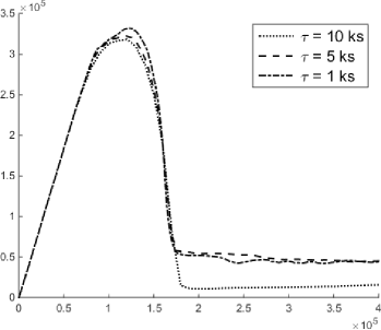
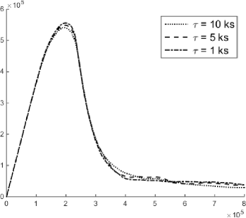
Fig. 4: Evolution of the reaction force corresponding to Figure 3; the time scales on the left and the right figures are different. Noteworthy, the force response is well converged even in situations when the energetics on Figure 3 exhibits still big gaps.

Dependence of the reaction-force evolution for varying viscosity of damage is shown in Figure 5 for $a_{2}$ as in Figures 3–4 compared also with a smaller viscosity $a_{2}=1\,$kPa s which already provides a response essentially identical to the even smaller viscosity $a_{2}=0.01\,$kPa s (not displayed in Figure 5) where conservation of energy is numerically still more difficult to achieve. This indicates a certain tendency for convergence towards the model using rate-independent damage combined with rate-dependent healing (as in [37, Sect. 5.2.7]) and with perfect plasticity, which is theoretically not justified, however.

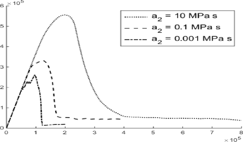
Fig. 5: Dependence of the repulsive-force response on the viscosity of damage, the cases $a_{2}=10$ and $0.1\,{\rm MPa\,s}$ are (parts of) Figure 4 and are here compared also with even less viscous damage for $a_{2}=1\,{\rm kPa\,s}$ which gives essentially the same response as for the nearly inviscid case $a_{2}=0.01\,{\rm kPa\,s}$ (not displayed, however); the time-step $\tau=1\,{\rm ks}$. For decreasing viscosity, the rupture occurs earlier and propagates faster, showing a tendency to converge to an inviscid rate-independent (and theoretically not justified) damage model.

Let us eventually remark that the a-posteriori information obtained from the residuum in the discrete energy balance (3.9c) written at a current time $t$ (as also used in Figure 3) can be used to control adaptively the time step in a way to keep the numerical error in the energy under an a-priori prescribed tolerance and, on the other hand, not to waste computational time by making too small time steps in periods of slow evolution. We intentionally presented our numerical simulation on equidistant time partitions, but for actual geophysical simulations with very big difference in time scale between fast damage (earthquakes) and very slow healing, such an adaptivity is necessary.

References

[1]
J. Alberty, C. Carstensen, and D. Zarrabi.
Adaptive numerical analysis in primal elastoplasticity with
hardening.
Comput. Methods Appl. Mech., 171:175–204, 1999.
[2]
R. Alessi, J.-J. Marigo, and S. Vidoli.
Gradient damage models coupled with plasticity and nucleation of
cohesive cracks.
Arch. Rational Mech. Anal., 214:575–615, 2014.
[3]
R. Alessi, J.-J. Marigo, and S. Vidoli.
Gradient damage models coupled with plasticity: Variational
formulation and main properties.
Mechanics of Materials, 2014.
[4]
L. Ambrosio, N. Fusco, and D. Pallara.
Functions of Bounded Variation and Free Discontinuity Problems.
Clarendon Press, Oxford, New York, 2000.
[5]
S. Bartels, A. Mielke, and T. Roubíček.
Quasistatic small-strain plasticity in the limit of vanishing
hardening and its numerical approximation.
SIAM J. Numer. Anal., 50:951–976, 2012.
[6]
M. Brokate, C. Carstensen, and J. Valdman.
A quasi-static boundary value problem in multi-surface
elastoplasticity. ii: Numerical solution.
Math. Methods Appl. Sci., 28:881–901, 2005.
[7]
M. Cermak, T. Kozubek, S. Sysala, and J. Valdman.
A TFETI domain decomposition solver for elastoplastic
problems.
Applied Mathematics and Computation, 231:634––653, 2014.
[8]
P. Colli and A. Visintin.
On a class of doubly nonlinear evolution equations.
Comm. Partial Differential Equations, 15:737–756, 1990.
[9]
V. Crismale.
Globally stable quasistatic evolution for a coupled
elastoplastic-damage model.
a preprint SISSA 34/2014/MATE, 2014.
[10]
V. Crismale and G. Lazzaroni.
Viscous approximation of quasistatic evolutions for a coupled
elastoplastic-damage model.
a preprint SISSA 05/2015/MATE, 2015.
[11]
G. Dal Maso, A. DeSimone, and M. Mora.
Quasistatic evolution problems for linearly elastic-perfectly plastic
materials.
Archive Ration. Mech. Anal., 180:237–291, 2006.
[12]
G. Dal Maso, A. DeSimone, and F. Solombrino.
Quasistatic evolution for Cam-Clay plasticity: a weak formulation
via viscoplastic regularization and time parametrization.
Calc. Var. Partial Diff. Eqns., 40:125–181, 2011.
[13]
G. Dal Maso, G. Francfort, and R. Toader.
Quasistatic crack growth in nonlinear elasticity.
Arch. Rational Mech. Anal., 176:165–225, 2005.
[14]
F. Ebobisse and B. Reddy.
Some mathematical problems in perfect plasticity.
Comput. Methods Appl. Mech. Engrg., 193:5071–5094, 2004.
[15]
G. Francfort and A. Giacomini.
Small strain heterogeneous elasto-plasticity revisited.
Communications on Pure and Appl. Math., 65:1185–1241, 2012.
[16]
M. Frémond.
Non-Smooth Thermomechanics.
Springer, Berlin, 2002.
[17]
E. Giusti.
Direct Methods in Calculus of Variations.
World Scientific, Singapore, 2003.
[18]
P. Grassl and M. Jirásek.
Plastic model with non-local damage applied to concrete.
Int. J. Numer. Anal. Meth. Geomech., 30:71–90, 2006.
[19]
P. Gruber, D. Knees, S. Nesenenko, and M. Thomas.
Analytical and numerical aspects of time-dependent models with
internal variables.
Zeitschrift f. angew. Math. und Mechanik, 90:861–902, 2010.
[20]
P. Gruber and J. Valdman.
Solution of one-time-step problems in elastoplasticity by a Slant
Newton Method.
SIAM J. Scientific Computing, 31:1558–1580, 2009.
[21]
G. Grün.
Degenerate parabolic equations of fourth order and a plasticity model
with nonlocal hardening.
Zeits. Anal. Anwendungen, 14:541–573, 1995.
[22]
M. Gurtin and A. Murdoch.
A continuum theory of elastic material surfaces.
Arch. Rat. Mech. Anal., 57:291–323, 1974.
[23]
Y. Hamiel, V. Lyakhovsky, and Y. Ben-Zion.
The elastic strain energy of damaged solids with applications to
non-linear deformation of crystalline rocks.
Pure Appl. Geophys., 168:2199–2210, 2011.
[24]
W. Han and B. Reddy.
Plasticity (Mathematical Theory and Numerical Analysis).
Springer, New York, 1999.
[25]
M. Jirásek and Z. P. Bažant.
Inelastic Analysis of Structures.
J.Wiley, Chichester, 2002.
[26]
C. Johnson.
Existence theorems for plasticity problems.
J. Math. Pures Appl., 55:431–444, 1976.
[27]
L. Kachanov.
Introduction to Continuum Damage Mechanics.
M. Nijhoff, Dordrecht, 1986.
[28]
D. Krajcinovic.
Damage mechanics.
Mechanics of Materials, 8:117–197, 1989.
[29]
J. Lemaitre.
A course on damage mechanics.
Springer, Berlin, 2nd edition, 1996.
[30]
J. Lemaitre and R. Desmorat.
Engineering Damage Mechanics – Ductile, Creep, Fatigue and
Brittle Failures.
Springer, Berlin, 2005.
[31]
M. Liu and J. Carter.
A structured Cam Clay model.
Canadian Geotech. J., 39:1313––1332, 2002.
[32]
V. Lyakhovsky, Y. Ben-Zion, and A. Agnon.
Distributed damage, faulting, and friction.
J. Geophysical Res., 102:27,635–27,649, 1997.
[33]
V. Lyakhovsky and V. Myasnikov.
On the behavior of elastic cracked solid.
Phys. Solid Earth, 10:71–75, 1984.
[34]
V. Lyakhovsky, Z. Reches, R. Weiberger, and T. Scott.
Nonlinear elastic behaviour of damaged rocks.
Geophys. J. Int., 130:157–166, 1997.
[35]
G. Maugin.
The Thermomechanics of Plasticity and Fracture.
Cambridge Univ. Press, Cambridge, 1992.
[36]
A. Mielke.
Evolution in rate-independent systems (Ch. 6).
In C. Dafermos and E. Feireisl, editors, Handbook of
Differential Equations, Evolutionary Equations, vol. 2, pages 461–559.
Elsevier B.V., Amsterdam, 2005.
[37]
A. Mielke and Roubíček.
Rate Intependent Systems: Theory and Application.
Springer, New York, 2015, ISBN 978-1-4939-2705-0.
[38]
A. Mielke, T. Roubíček, and J. Zeman.
Complete damage in elastic and viscoelastic media and its energetics.
Comput. Methods Appl. Mech. Engrg., 199:1242–1253, 2010.
[39]
A. Mielke and F. Theil.
On rate-independent hysteresis models.
Nonlin. Diff. Eq. Appl., 11:151–189, 2004.
[40]
P. Podio-Guidugli.
Contact interactions, stress, and material symmetry, for nonsimple
elastic materials.
Theor. Appl. Mech., 28-29:261–276, 2002.
[41]
P. Podio-Guidugli, T. Roubíček, and G. Tomassetti.
A thermodynamically-consistent theory of the ferro/paramagnetic
transition.
Archive Rat. Mech. Anal., 198:1057–1094, 2010.
[42]
P. Podio-Guidugli and M. Vianello.
Hypertractions and hyperstresses convey the same mechanical
information.
Cont. Mech. Thermodynam., 22:163–176, 2010.
[43]
T. Rahman and J. Valdman.
Fast MATLAB assembly of FEM matrices in 2D and 3D: nodal
elements.
Appl.Math.Comput, 219:7151–7158, 2013.
[44]
S. Repin.
Errors of finite element method for perfectly elasto-plastic
problems.
Math. Models Methods Appl. Sci., 6:587–607, 1996.
[45]
T. Roubíček.
Rate independent processes in viscous solids at small strains.
Math. Meth. Appl. Sci., 32:825–862, 2009.
Erratum p. 2176.
[46]
T. Roubíček.
Nonlinear Partial Differential Equations with Applications.
Birkhäuser, Basel, 2nd edition, 2013.
[47]
T. Roubíček.
Thermodynamics of perfect plasticity.
Discrete and Cont. Dynam. Syst. - S, 6:193–214, 2013.
[48]
T. Roubíček, O. Souček, and R. Vodička.
A model of rupturing lithospheric faults with re-occurring
earthquakes.
SIAM J. Appl. Math., 73:1460–1488, 2013.
[49]
T. Roubíček and U. Stefanelli.
Magnetic shape-memory alloys: thermomechanical modeling and analysis.
Cont. Mech. Thermodynamics, 26:783–810, 2014.
[50]
M. Šilhavý.
Phase transitions in non-simple bodies.
Archive Rat. Mech. Anal., 88:135–161, 1985.
[51]
M. Sofonea, W. Han, and M. Shillor.
Analysis and approximation of contact problems with adhesion or