Kernel Machines for Current Status Data

Abstract

In survival analysis, estimating the failure time distribution is an important and difficult task, since usually the data is subject to censoring. Specifically, in this paper we consider current status data, a type of data where all of the observations are censored. The format of the data is such that the failure time is restricted to knowledge of whether or not the failure time exceeds a random monitoring time. We propose a flexible kernel machine approach for estimation of the failure time expectation as a function of the covariates, with current status data. In order to obtain the kernel machine decision function, we minimize a regularized version of the empirical risk with respect to a new loss function. Using finite sample bounds and novel oracle inequalities, we prove that the obtained estimator converges to the true conditional expectation for a large family of probability measures. Finally, we present a simulation study and an analysis of real-world data that compares the performance of the proposed approach to existing methods. We show empirically that our approach is comparable to current state of the art, and in some cases is even better.

T1The authors were funded in part by NSF grant DMS-1407732.

Yael Travis-Lumerlabel=e1]travis-lumer@campus.technion.ac.il and Yair Goldberglabel=e2]yairgo@technion.ac.il

1 Introduction

In this paper we aim to develop a general model free method for analyzing current status data using machine learning techniques. In particular, we propose a kernel machine learning method for estimation of the failure time expectation with current status data. Kernel machines, also known as support vector machines, were originally introduced by Vapnik in the 1990’s and are firmly related to statistical learning theory (Vapnik, 1999). Kernel machines are learning algorithms that utilize positive definite kernels (Hofmann et al., 2008). The choice of kernel machines for current status data is motivated by the fact that kernel machines can be implemented easily, have fast training speed, produce decision functions that have a strong generalization ability, and can guarantee convergence to the optimal solution, under some weak assumptions (Shivaswamy et al., 2007).

The format of current status data is such that the failure time $T$ is restricted to knowledge of whether or not $T$ exceeds a random monitoring time $C$. This data format is quite common and includes examples from various fields. Jewell and van der Laan (2004) mention a few examples including: studying the distribution of the age of a child at weaning given observation points; when conducting a partner study of HIV infection over a number of clinic visits; and when a tumor under investigation is occult and an animal is sacrificed at a certain time point in order to determine presence or absence of the tumor. For instance, in the last example, when performing carcinogenicity testing, $T$ is the time from exposure to a carcinogen and until the presence of a tumor, and $C$ is the time point at which the animal is sacrificed in order to determine presence or absence of the tumor. Clearly, it is difficult to estimate the failure time distribution since we cannot observe the failure time $T$. These examples illustrate the importance of this topic and the need to find advanced tools for analyzing such data.

There are several approaches for analyzing current status data. Traditional methods include parametric models where the underlying distribution of the survival time is assumed to be known, such as Weibull, Gamma, and other distributions with non-negative support. Other approaches include semiparametric models, such as the Cox proportional hazards model, and the accelerated failure time (AFT) model (see, for example, Klein and Moeschberger, 2005). Several works including Diamond et al. (1986), Shiboski and Jewell (1992), Jewell and van der Laan (2004) and others, have suggested the Cox proportional hazard model for current status data, where the Cox model can be represented as a generalized linear model with a log-log link function. Other works, including Tian and Cai (2006), discussed the use of the AFT model for current status data and suggested different algorithms for estimating the model parameters. Additional semiparametric regression models for current status data include proportional odds (Rossini and Tsiatis, 1996), additive hazards (Lin et al., 1998), additive transformations (Cheng and Wang, 2011), linear transformations (Sun and Sun, 2005), and linear regression (Shen, 2000). Needless to say that both parametric and semiparametric models demand stringent assumptions on the distribution of interest which can be restrictive. For this reason, additional estimation methods are needed.

Nonparametric methods for analyzing current status data were also investigated in the literature. Nonparametric maximum likelihood estimation (NPMLE) of the failure time distribution function is commonly used with this type of data, and relies on the PAV algorithm of Ayer et al. (1955). Burr and Gomatam (2002) studied nonparametric estimation of the conditional distribution function of the failure time given the covariates, based on a locally smoothed modification of the NPMLE. Wang et al. (2012) studied nonparametric estimation of the marginal distribution function of the failure time using the copula model approach. Honda (2004) constructed an estimator for the regression function utilizing a modification of maximum rank correlation, and estimated the difference between the regression function at some value, to the regression function at a standard fixed point. Note that these works are not specifically intended for estimation of the conditional expectation and thus might not yield accurate estimates.

Over the past two decades, some learning algorithms for censored data have been proposed. However, most of these algorithms cannot be applied to current status data but only to other, more common, censored data formats. Recently, several authors suggested the use of kernel machines, or similarly support vector machines, for survival data, including Van Belle et al. (2007), Khan and Zubek (2008), Eleuteri and Taktak (2011), Goldberg and Kosorok (2017), Shiao and Cherkassky (2013), Wang et al. (2016), and Pölsterl et al. (2016). These examples illustrate that initial steps in this direction have already been taken. However, as far as we know, the only work based on kernel machines that can also be applied to current status data is by Shivaswamy et al. (2007) which has a more computational and less theoretic nature. The authors studied the use of kernel machines for regression problems with interval censoring and, using simulations, showed that the method is comparable to other missing data tools.

We present a kernel machine framework for current status data. We propose a learning method, denoted by KM-CSD, for estimation of the failure time conditional expectation. We investigate the theoretical properties of the KM-CSD, and in particular, prove consistency for a large family of probability measures. In order to estimate the conditional expectation we use a modified version of the quadratic loss, using the methodology of van der Laan and Robins (1998, 2003). Since the failure time $T$ is not observed, our new modified loss function is based on the censoring time $C$ and on the current status indicator. Finally, in order to obtain the KM-CSD estimator, we minimize a regularized version of the empirical risk with respect to our new proposed loss. Note that the terminology decision function is used in the kernel machine context to describe the obtained estimator.

The kernel machine we present in this work may be referred to as an inverse probability weighted complete-case estimator (van der Laan and Robins 2003, Tsiatis 2006, Chapter 6). It is tempting to use the tools described in these books to derive doubly-robust kernel machine estimators. In the context of estimating equations with missing data, doubly-robust estimators are typically constructed by adding an augmentation term. This term is constructed by projecting the estimating equation onto the augmentation space (see Tsiatis 2006, Section 7.4, and Theorem 10.1). However, in our kernel machine setting, the estimator is obtained as the minimizer of a weighted loss function over a reproducing kernel Hilbert space (RKHS) and thus it is not clear how meaningful it is to project the loss function on the augmentation space. It is also not trivial to add a term to the proposed regularized empirical risk minimization problem in a way that yields a convex optimization problem over an RKHS, which is essential for deriving the results presented in this paper. While doubly-robust estimators for current status data were derived in the semiparametric literature (Andrews et al. 2005), we do not consider such estimators in this work. To the best of our knowledge, the only work that studied doubly-robust estimators in the context of kernel machines was done by Liu and Goldberg (2018), however this was done in the context of missing responses, and cannot be applied to our case.

The contribution of this work includes the development of a nonparametric estimator of the conditional expectation, the development of a kernel machine framework for current status data, the development of new oracle inequalities for censored data, and the study of the theoretical properties and the consistency of the KM-CSD.

The paper is organized as follows. In Section 2 we describe the formal setting of current status data and discuss the choice of the quadratic loss for estimating the conditional expectation. In Section 3 we present the proposed KM-CSD and its corresponding loss function. Section 4 contains the main theoretical results, including finite sample bounds and consistency. Section 5 contains the simulations and Section 6 contains an analysis of real world data. Concluding remarks are presented in Section 7. The proofs appear in Proofs. The Matlab code for both the algorithm and for the simulations, as well as the artificially censored data from Section 6.2, can be found in the Supplementary Materials.

2 Preliminaries

In this section we present the notation used throughout the paper. First we describe the data setting and then we discuss briefly loss functions and risks.

Assume that the data consists of $n$ independent and identically distributed random triplets $D=\{(Z_{1},C_{1},\Delta_{1}),\\ \ldots,\allowbreak(Z_{n},C_{n},\Delta_{n})\}$. The random vector $Z$ is a vector of covariates that takes its values in a compact set $\mathcal{Z}\subset\mathbb{\mathbb{R}}^{d}$. The failure-time $T$ is non-negative, the random variable $C$ is the non-negative censoring time, where both $C$ and $T$ are contained in the interval $[0,\tau]\equiv\mathcal{Y},$ for some constant $\tau>0$. The indicator $\Delta=\mathbf{{1}}\{T\leq C\}$ is the current status indicator at time $C$, obtaining the value 1 when $T\leq C$, and 0 otherwise. For example, in carcinogenicity testing, an animal is sacrificed at a certain time point in order to determine presence or absence of the tumor. In this example, $T$ is the time from exposure to a carcinogen and until the presence of a tumor, $Z$ can be any explanatory information collected such as the weight of the animal, $C$ is the time point at which the animal is sacrificed, and $\Delta$ is the current status indicator at time $C$ (indicating whether the tumor has developed before the censoring time, or not).

We now move to discuss a few definitions of loss functions and risks, following Steinwart and Christmann (2008). Let$\left(\mathcal{\mathcal{Z}},\mathcal{A}\right)$ be a measurable space and $\mathcal{Y}\subset\mathbb{\mathbb{R}}$ be a closed subset. Then a loss function is any measurable function $L$ from $\mathcal{Y}\times\mathbb{R}$ to $[0,\infty)$.

Let $L:\mathcal{Y}\times\mathbb{R}\rightarrow[0,\infty)$ be a loss function and $P$ be a probability measure on $\mathcal{Z\times Y}$. For a measurable function $f:\mathcal{Z}\mapsto\mathbb{\mathbb{R}}$, the $L$-risk of $f$ is defined by $R_{L,P}\left(f\right)\equiv E_{P}\left[L\left(Y,f(Z)\right)\right]=\int_{Z\times Y}L\left(y,f(z)\right)dP(z,y)$. A function $f$ that achieves the minimum $L$-risk is called a Bayes decision function and is denoted by $f^{*}$, and the minimal $L$-risk is called the Bayes risk and is denoted by $R_{L,P}^{*}$. Finally, the empirical $L$-risk is defined by $R_{L,D}\left(f\right)=\frac{1}{n}{\displaystyle\sum_{i=1}^{n}}L(y_{i},f(z_{i}))$. It is well known (see, for example, Hastie et al., 2013) that the conditional expectation is the Bayes decision function with respect to the quadratic loss. That is, $E[Y|Z]=f^{*}=\operatorname*{argmin}_{f}R_{L,P}(f)$, where $L$ is the quadratic loss defined by $L(Y,f(Z))=(Y-f(Z))^{2}$.

Recall that our goal is to estimate the conditional expectation of the failure-time $T$ given the covariates $Z$. However, in the setting of current status data, the response variable (failure-time) is not observed, making the estimation procedure more complex. It is not even clear if and how loss functions can be defined with current status data. In the following section we construct a new modification of the quadratic loss that is based on the censoring time and on the current status indicator, and use it to estimate the conditional expectation of the unobservable failure-time.

3 Kernel Machines for Current Status Data

This section is divided into three subsections. We start by describing general kernel machines for uncensored data. Then we define a new loss function for current status data, utilizing an equality between risks, and incorporate it into the kernel machine framework. Finally we define the proposed estimator of the conditional expectation of the failure-time, with current status data, and discuss some assumptions regarding the censoring mechanism.

3.1 Kernel Machines for Uncensored Data

Let $\mathcal{H}$ be a reproducing kernel Hilbert space (RKHS) of functions from $\mathcal{Z}$ to $\mathbb{R}$, where an RKHS is a function space that can be characterized by some kernel function $k:\mathcal{Z}\times\mathcal{Z}\mapsto\mathbb{R}$. For more information on reproducing kernel Hilbert spaces, we refer the reader to Steinwart and Christmann 2008, Chapter 4. A continuous kernel $k$ for which the corresponding RKHS $\mathcal{H}$ is dense in the space of continuous functions on $\mathcal{Z}$, $C(\mathcal{Z})$, is called a universal kernel (see, for example, Steinwart and Christmann 2008, Definition 4.52). Fix such an RKHS $\mathcal{H}$ and denote its norm by $\left\|\cdot\right\|_{\mathcal{H}}$. Let $\{\lambda_{n}\}>0$ be some sequence of regularization constants. A kernel machine decision function for uncensored data is defined by:

$$f_{D,\lambda_{n}}=\arg\min{}_{f\in\mathcal{H}}\lambda_{n}\|f\|_{\mathcal{H}}^{2}+\frac{1}{n}\sum_{i=1}^{n}L(T_{i},f(Z_{i}))\,.$$

3.2 Equality Between Risks

In this subsection we show that the risk can be represented as the sum of two terms

$$E\left[\frac{(1-\Delta)\ell(C,f(Z))}{g(C|Z)}\right]+E[L(0,f(Z))].$$

We recall that current status data consists of $n$ independent and identically-distributed random triplets $D=\{(Z_{1},C_{1},\Delta_{1}),\ldots,(Z_{n},C_{n},\Delta_{n})\}$.

Let $F(\cdot|Z=z)$ and $G(\cdot|Z=z)$ be the cumulative distribution functions of the failure time and censoring, respectively, given the covariates $Z=z$. Let $g(\cdot|Z=z)$ be the density of $G(\cdot|Z=z)$. Throughout this work we will assume the following:

1. The censoring time $C$ is independent of the failure time $T$ given the covariates $Z$.

2. $C$ and $T$ take values in the interval $[0,\tau]\equiv\mathcal{Y}$ and $\underset{{}_{z\in\mathcal{Z},c\in\mathcal{Y}}}{\inf}g\left(c|z\right)\geq 2\kappa>0$, for some $\kappa>0$.

The conditional independence assumption (A1) is a standard identifiability assumption in survival analysis (see, for example, Klein and Goel 1992 and Klein and Moeschberger 2005). Assumption (A2) is needed in order to guarantee that integration with respect to $T$ and $C$ can be exchanged, and in order to allow for division by the censoring density. Similar assumptions were made by van der Laan and Robins (1998).

For current status data, we introduce the following identity between risks, following van der Laan and Robins (1998, 2003). We extend this identity by incorporating loss functions and covariates. Let $L:\mathcal{Y}\times\mathbb{\mathbb{R}}\mapsto[0,\infty)$ be a loss function differentiable in the first variable. Let $\ell:\mathcal{Y}\times\mathbb{\mathbb{R}}\mapsto\mathbb{\mathbb{R}}$ be the derivative of $L$ with respect to the first variable.

We would like to find the minimizer of $R_{L,P}(f)$ over a set $\mathcal{H}$ of functions $f$. Note that

$$R_{L,P}(f)\equiv E_{Z}E_{T|Z}L(T,f(Z))=E_{Z}\left[\int_{0}^{\tau}L(t,f(Z))dF(t|Z)\right]$$

$$= E_{Z}\left[\int_{0}^{\tau}\ell(t,f(Z))(1-F(t|Z))dt-\left.L(t,f(Z))(1-F(t|Z))\right|_{0}^{\tau}\right]$$

$$= E_{Z}\left[\int_{0}^{\tau}\ell(t,f(Z))(1-F(t|Z))dt\right]+E[L(0,f(Z))]\,,$$

and that $(1-\Delta)=\mathbf{{1}}\{T>C\}$ and thus

$$E\left[\frac{(1-\Delta)\ell(C,f(Z))}{g(C|Z)}\right]= E_{Z,T}\left[E_{C}\left[\left.\frac{\mathbf{{1}}\{T>C\}\ell(C,f(Z))}{g(C|Z)}\right|Z,T\right]\right]$$

$$= E_{Z,T}\left[\int_{0}^{\tau}\frac{\mathbf{{1}}\{T>c\}\ell(c,f(Z))g(c|Z)}{g(c|Z)}dc\right]$$

$$= E_{Z,T}\left[\int_{0}^{\tau}\mathbf{{1}}\{T>c\}\ell(c,f(Z))dc\right]$$

$$= E_{Z}\left[\int_{0}^{\tau}\ell(c,f(Z))\int_{0}^{\tau}\mathbf{{1}}\{t>c\}dF(t|Z)dc\right]$$

$$= E_{Z}\left[\int_{0}^{\tau}\ell(c,f(Z))(1-F(c|Z))dc\right]\,.$$

3.3 Kernel Machines for Current Status Data

Hence, in order to estimate the minimizer of $R_{L,P}(f)$, one can minimize a regularized version of the empirical risk with respect to a new loss function defined by

$$L^{n}(D,(Z,C,\Delta,s))=\frac{(1-\Delta)\ell(C,s)}{g(C|Z)}+L(0,s)\,.$$

Note that this function need not be convex nor a loss function. Recall that we are interested in estimating the conditional expectation. This means that we would like to minimize the risk with respect to the quadratic loss. For the quadratic loss, our new loss function becomes

$$L^{n}(D,(Z,C,\Delta,s))=\frac{(1-\Delta)2(C-s)}{g(C|Z)}+s^{2}\,.$$

Note that this function is convex but not necessarily a loss function since it can obtain negative values. However, one can always add a constant to ensure positivity. Since this constant does not effect optimization it will be neglected hereafter. For a detailed explanation, see Appendix B.

In order to implement this result into the kernel machine framework, we propose to define the KM-CSD decision function for current status data by

$$f_{D,\lambda}=\arg\min{}_{f\in\mathcal{H}}\lambda\|f\|_{\mathcal{H}}^{2}+\frac{1}{n}{\displaystyle\sum_{i=1}^{n}}\left[\frac{(1-\Delta_{i})2(C_{i}-f(Z_{i}))}{g(C_{i}|Z_{i})}+(f(Z_{i}))^{2}\right].$$ (1)

Explicit computation of the decision function can be found in Appendix A. Note that if the censoring mechanism is unknown, we can replace the density $g$ in Eq. 1 with its estimate $\hat{g}$, as long as $\hat{g}$ is strictly positive on $[0,\tau]\equiv\mathcal{Y}$; in this case the kernel machine decision function is

$$f_{D,\lambda}=\arg\min{}_{f\in\mathcal{H}}\lambda\|f\|_{\mathcal{H}}^{2}+\frac{1}{n}{\displaystyle\sum_{i=1}^{n}}\left[\frac{(1-\Delta_{i})2(C_{i}-f(Z_{i}))}{\hat{g}(C_{i}|Z_{i})}+(f(Z_{i}))^{2}\right]$$

(note the use of $\hat{g}$ instead of $g$ in the denominator).

We note that for current status data, the assumption of some knowledge of the censoring distribution is reasonable, for example, when it is chosen by the researcher (Jewell and van der Laan, 2004). In other cases, the density can be estimated using either parametric or nonparametric density estimation techniques such as kernel estimates. It should be noted that the censoring variable itself is fully observed (not censored) and thus simple density estimation techniques can be used in order to estimate the density $g$.

4 Theoretical Results

The main goal of our work is to find a ‘good’ estimator of the failure time conditional expectation. A good estimator should first and foremost be consistent, that is, its risk should converge in probability to the Bayes risk. Additionally, we would like such an estimator to be consistent for a large family of probability measures. The consistency proof is based on novel oracle inequalities that are presented below.

We start by proving risk consistency of the KM-CSD learning method for a large family of probability measures. We first assume that the censoring mechanism is known, which means that the true density of the censoring variable $g$ is known. Using this assumption, and some additional conditions, we bound the difference between the risk of the KM-CSD decision function and the Bayes risk in order to form finite sample bounds. We use this result to show that the KM-CSD converges in probability to the Bayes risk. That is, we demonstrate that for a large family of probability measures, the KM-CSD learning method is consistent. We then consider the case in which the censoring mechanism is unknown, and thus the density $g$ needs to be estimated. We estimate the density $g$ using nonparametric kernel density estimation, and develop a novel finite sample bound. We use this bound to prove that the KM-CSD is consistent even when the censoring distribution is unknown.

For simplicity, we use the normalized version of the quadratic loss.

Definition 1.

Let $L(y,s)=\frac{(y-s)^{2}}{\tau^{2}}$ be the normalized quadratic loss, let $l(y,s)=\frac{2(y-s)}{\tau^{2}}$ be its derivative with respect to the first variable, and let $L^{n}(D,(Z,C,\Delta,s))=\frac{1}{\tau^{2}}\left(\frac{(1-\Delta)2(C-s)}{g(C|Z)}+s^{2}\right)$ be the proposed modified version of this loss.

Since both $L$ and $l$ are convex functions with respect to $s$, then for any compact set $\mathcal{S}=[-S,S]\subset\mathbb{R}$, Both $L$ and $l$ are bounded and Lipschitz continuous with constants $c_{L}$ and $c_{l}$ that depend on $\mathcal{S}$.

Remark 1.

$L(y,0)\leq 1$ for all $y\in\mathcal{Y}$ and $\ell(y,s)\leq B_{1}$ for all $(y,s)\in\mathcal{Y\times S}$ and for some constant $B_{1}>0$.

We need the following additional assumptions:

1. $\mathcal{Z}\subset\mathbb{\mathbb{R}}^{d}$ is compact,

2. $\mathcal{H}$ is an RKHS of a continuous kernel $k$ with $\left\|k\right\|_{\infty}\leq 1$.

Assumptions (A3-A4) are standard technical assumptions in the kernel machines literature.

Define the approximation error by $A_{2}(\lambda)=\underset{f\in\mathcal{H}}{\inf}\lambda\left\|f\right\|_{\mathcal{H}}^{2}+R_{L,P}(f)-R_{L,P}^{*}$. Define $B_{2}=c_{L}\lambda^{-\nicefrac{{1}}{{2}}}+1$ and $B=\frac{B_{1}}{2\kappa}+B_{2}$, where $B_{1}$ is defined in Remark 1, $\kappa$ is defined in Assumption (A2), $c_{L}$ is the Lipschitz constant of the normalized quadratic loss $L$, and $\lambda$ is the regularization parameter.

4.1 Case I - The Censoring Density $g$ is Known

In this section we develop finite sample bounds assuming that the censoring density $g$ is known.

Theorem 1.

Assume that (A1)-(A4) hold. Then for fixed $\lambda>0,\,n\geq 1,\,\varepsilon>0$, and $\theta>0$, with probability not less than $1-\exp(-\theta)$

$$\lambda\left\|f_{D,\lambda}\right\|_{\mathcal{H}}^{2}+R_{L,P}(f_{D,\lambda})-R_{L,P}^{*}-A_{2}(\lambda)\\ \leq B\sqrt{\frac{2\log\left(2N(\sqrt{\frac{1}{\lambda}}B_{H},\left\|\cdot\right\|_{\infty},\epsilon)\right)+2\theta}{n}}+\frac{2c_{l}\varepsilon}{\kappa}+4c_{L}\varepsilon$$

where $N(\lambda^{-\frac{1}{2}}B_{H},\left\|\cdot\right\|_{\infty},\epsilon)$ is the covering number of the $\varepsilon-net$ of $\sqrt{\frac{1}{\lambda}}\overline{B_{H}}$ with respect to supremum norm and where $\overline{B_{H}}$ is the closure of the unit ball of $\mathcal{H}$ (for further details see Steinwart and Christmann 2008) .

The proof of this theorem appears in Appendix C.1.

We now move to discuss consistency of the KM-CSD learning method. By definition, $P$-universal consistency means that for any $\epsilon>0$,

$$\underset{n\rightarrow\infty}{\lim}P(D\in(\mathcal{Z\times\mathcal{Y}})^{n}\,:\,R_{L,P}(f_{D,\lambda_{n}})\leq R_{L,P}^{*}+\epsilon)=1,$$ (2)

where $R_{L,P}^{*}$ is the Bayes risk. Universal consistency means that (2) holds for all probability measures $P$ on $\mathcal{Z\times Y}$. However, in survival analysis we have the problem of identifiability and thus we will limit our discussion to probability measures that satisfy some identification conditions. Let $\mathcal{P}$ be the set of all probability measures that satisfy Assumptions (A1)-(A2). We say that a learning method is $\mathcal{P}$-universal consistent when (2) holds for all probability measures $P\in\mathcal{P}$.

In order to show $\mathcal{P}$-universal consistency, we utilize the finite sample bounds of Theorem 1. The following assumption is also needed for proving $\mathcal{P}$-universal consistency:

1. $k$ is a universal kernel.

Universal kernels are a wide family of kernel functions that include Gaussian and Taylor kernels. A kernel $k$ is called universal if the RKHS $\mathcal{H}$ of $k$ is dense in the space of continuous functions on $\mathcal{Z}$, $C(\mathcal{Z})$, with respect to the sup norm. Assumption (A5) means that $\underset{f\in\mathcal{H}}{\inf}R_{L,P}(f)=R_{L,P}^{*}$, for all probability measures $P$ on $\mathcal{Z\times Y}$.

Corollary 1.

Assume the setting of Theorem 1 and that Assumption (A5) holds. Assume that there exist constants $a\geq 1$ and $p>0$ such that $\log\left(N(B_{H},\left\|\cdot\right\|_{\infty},\epsilon)\right)\leq a\epsilon^{-2p}$. Let $\lambda_{n}$ be a sequence such that $\lambda_{n}\underset{n\rightarrow\infty}{\rightarrow}0$ and $\lambda_{n}^{1+p}n\underset{n\rightarrow\infty}{\rightarrow}\infty.$ Then the KM-CSD learning method is $\mathcal{P}$-universal consistent.

The proof of this theorem appears in Appendix C.2.

Note that the bound on the covering number $N(B_{H},\left\|\cdot\right\|_{\infty},\epsilon)$ in Corollary 1 is satisfied for smooth kernels, such as polynomial and Gaussian kernels, for arbitrarily small $p>0$ (see Steinwart and Christmann 2008, Section 6.4).

4.2 Case II - The Censoring Density $g$ is Unknown

Here we consider the case in which the censoring mechanism is unknown, and thus the density $g$ needs to be estimated. We estimate the density $g$ using nonparametric kernel density estimation, and develop a novel finite sample bound. We use this bound to prove that the KM-CSD is consistent even when the censoring distribution is unknown. Note that asymptotic results for kernel density estimators are well known in the literature (see, for example, Silverman 1978). However, to the best of our knowledge, finite sample bounds for this case do not exist and hence are developed here.

For simplicity, we assume here that the censoring time $C$ is independent of the covariates $Z$. One can generalize the estimation procedure to include dependence of the censoring time $C$ on the covariates $Z$; for example, the conditional density estimate can be computed by the ratio of the joint density estimate to the marginal density estimate. In Lemma 1 we construct finite sample bounds on the difference between the estimated density $\hat{g}$ and the true density $g$. In Theorem 2 we utilize this bound to form finite sample bounds for the KM-CSD learning method.

Definition 2.

We say that $K_{m}:\mathbb{\mathbb{R}\mapsto R}$ (not to be confused with the kernel function $k$ of the RKHS $\mathcal{H})$ is a kernel of order $m$, if the functions $u\mapsto u^{j}K_{m}(u)\,\,,j=0,1,...,m$ are integrable and satisfy $\int_{-\infty}^{\infty}K_{m}(u)du=1$ and $\int_{-\infty}^{\infty}u^{j}K_{m}(u)du=0,\,\,j=1,...,m$.

Definition 3.

The Hölder class $\sum(\beta,\mathcal{L})$ of functions $f:\mathbb{\mathbb{R}\mapsto R}$ is the set of $m=\left\lfloor\beta\right\rfloor$ times differentiable functions whose derivative $f^{(m)}$ satisfies $\left|f^{(m)}(x)-f^{(m)}(x^{\prime})\right|\leq\mathcal{L}\left|x-x^{\prime}\right|^{\beta-m}$ for any $x,x^{\prime}\in\mathbb{R}$ and for some constant $\mathcal{L}>0$.

Lemma 1.

Let $K_{m}:\mathbb{\mathbb{R}\mapsto R}$ be a kernel function of order $m=\left\lfloor\beta\right\rfloor$ satisfying $\int_{-\infty}^{\infty}K_{m}^{2}(u)du<\infty$ and define $\hat{g}(x)=(hn)^{-1}\stackrel{{\scriptstyle}}{{\sum_{i=1}^{n}K_{m}\left((C_{i}-x)/h\right)}}$ where $h$ is the bandwidth. Suppose that the true density $g$ and its estimate $\hat{g}$ both satisfy $g(c),\hat{g}(c)\leq g_{max}<\infty$. Let us also assume that $g(c)$ belongs to the $\mathrm{H\ddot{o}lder}$ class $\sum(\beta,\mathcal{L})$. Finally, assume that $\int_{-\infty}^{\infty}\left|u\right|^{\beta}\left|K_{m}(u)\right|du<\infty$. Then for any $\theta>0$,

$$Pr\left(\frac{1}{n}\sum_{i=1}^{n}\left|\hat{g}(C_{i})-g(C_{i})\right|>\sqrt{\frac{2D_{1}\theta}{n^{2}h}}+\frac{2g_{max}\theta}{3n}+D_{2}\cdot h^{\beta}\right)\leq\exp(-\theta)$$

where $D_{1}=g_{max}\int_{-\infty}^{\infty}K_{m}^{2}\left(v\right)dv$ and $D_{2}=\mathcal{L}\left|\pi\right|^{\beta-m}/m!\int_{-\infty}^{\infty}{\left|K_{m}\left(v\right)\right|}\left|v\right|^{\beta}dv$ are constants, and for some $\pi\in[0,1]$.

The proof of the lemma is based on Tsybakov (2008, Propositions 1.1 and 1.2) together with basic concentration inequalities; the proof can be found in Appendix C.3.

We now move to construct finite sample bounds for the KM-CSD learning method when $g$ is unknown using the above lemma. We assume that $\hat{g}$ is the kernel density estimate of $g,$ such that the conditions of Lemma 1 hold.

Theorem 2.

Assume that (A1)-(A4) hold. Assume the setting of Lemma 1 and that $\underset{{}_{z\in\mathcal{Z},c\in C}}{\inf}\hat{g}\left(c\right)\geq\kappa>0,$ for some $\kappa>0$. Then for fixed $\lambda>0,\,\theta>0,\,n\geq 1,\,\varepsilon>0$, we have with probability not less than $1-2\exp(-\theta)$ that

$$\lambda\left\|f_{D,\lambda}\right\|_{\mathcal{H}}^{2}+R_{L,P}(f_{D,\lambda})-R_{L,P}^{*}-A_{2}(\lambda)\leq B\sqrt{\frac{2log\left(2N(\sqrt{\frac{1}{\lambda}}B_{H},\left\|\cdot\right\|_{\infty},\epsilon)\right)+2\theta}{n}}+\frac{3c_{l}\varepsilon}{\kappa}+4c_{L}\varepsilon+2\eta$$

where $\eta\equiv\frac{B_{1}}{2\kappa^{2}}\left(\sqrt{\frac{2D_{1}\theta}{n^{2}h}}+\frac{2g_{max}\theta}{3n}+D_{2}\cdot h^{\beta}\right)$.

The proof of the theorem appears in Appendix C.4.

Using the above theorem we show that under some mild conditions, the KM-CSD decision function converges in probability to the conditional expectation.

Corollary 2.

Assume the setting of Theorem 2 and assume that Assumption (A5) holds. Assume that there exist constants $a\geq 1$ and $p>0$ such that $\log\left(N(B_{H},\left\|\cdot\right\|_{\infty},\epsilon)\right)\\ \leq a\epsilon^{-2p}$. Let $\lambda_{n}$ be a sequence such that $\lambda_{n}\underset{n\rightarrow\infty}{\rightarrow}0$ and that $\lambda_{n}^{1+p}n\underset{n\rightarrow\infty}{\rightarrow}\infty.$ Then the KM-CSD learning method is $\mathcal{P}$-universal consistent.

The proof of this theorem appears in Appendix C.5.

We refer the readers to Appendix D for a straightforward derivation of learning rates that are based on the same oracle inequalities of Theorem 1 and 2.

5 Simulation Study

We test the KM-CSD learning method on simulated data and compare its performance to current state of the art. We construct four different data-generating mechanisms, including one-dimensional and multi-dimensional settings. For each data type, we compute the difference between the KM-CSD decision function and the true expectation. We compare this result to results obtained by the Cox model and by the AFT model. We were not able to gain access to other nonparametric methods and hence will not compare them to our approach. As a reference, we compare all these methods to the Bayes risk, which we calculated for the simulations.

For each data setting, we considered two cases: (i) the censoring density $g$ is known; and (ii) the censoring density is unknown. For the second setting, the distribution of the censoring variable was estimated using univariate nonparametric kernel density estimation with a Gaussian kernel. For simplicity, we assumed that the censoring time $C$ is independent of the covariates $Z$. The code was written in Matlab, using the Spider library. In order to fit the Cox model to current status data, we downloaded the ‘ICsurv’ R package (McMahan and Wang, 2014). In this package, monotone splines are used to estimate the cumulative baseline hazard function, and the model parameters are then chosen via the EM algorithm. We chose the most commonly used cubic splines. To choose the number and locations of the knots, we followed Ramsay (1988) and McMahan et al. (2013) who both suggested using a fixed small number of knots and thus we placed the knots evenly at the quartiles. For the AFT model, we used the ‘surv reg’ function in the ‘Survival’ R package (Therneau and Lumley, 2016). In order to call R through Matlab, we installed the R package rscproxy (Baier, 2012), installed the statconnDCOM server (Baier and Neuwirth, 2007), and download the Matlab R-Link toolbox (Henson, 2004). For the kernel of the RKHS $\mathcal{H}$, we used both a linear kernel and a Gaussian RBF kernel $k(x_{i},x_{j})=\exp\left(\left\|x_{i}-x_{j}\right\|_{2}^{2}/2\sigma^{2}\right)$, where $\sigma$ and $\lambda$ were chosen using 5-fold cross-validation. Cross validation is commonly used for kernel machine parameter selection (see, for example, Steinwart and Christmann 2008). van der Vaart et al. (2006) developed oracle inequalities for penalized risk minimization with multi-fold cross validation. This result can be applied to kernel machines and justifies the use of cross validation for parameter selection. Since in our case the failure time $T$ is not observed, using cross-validation with current status data is not trivial. However, one can use cross-validation with respect to our proposed loss. Recall that the risk with respect to the original loss function equals to the risk with respect to our proposed loss function. Hence we used 5-fold cross-validation with respect to the empirical risk obtained by our proposed loss. The code for the algorithm and for the simulations can be found in the Supplementary Materials.

We consider the following four failure time distributions, corresponding to the four different data-generating mechanisms: (1) Weibull, (2) Multi-Weibull, (3) Multi-Log-Normal, and (4) an additional example where the failure time expectation is triangle shaped. We present below the KM-CSD risks for each case and compare them to risks obtained by other methods. The risks are based on 100 iterations per sample size. The Bayes risk is also plotted as a reference. The Bayes risk was calculated based on the Monte Carlo method where a large number of observations were drawn from the true failure time distribution; the empirical risk was then calculated.

In Setting 1 (Weibull failure-time), the covariates $Z$ are generated uniformly on $[0,1],$ the censoring variables $C$ is generated uniformly on $[0,\tau],$ and the failure time $T$ is generated from a Weibull distribution with parameters $scale=\exp(-0.5Z),\,shape=2$. The failure time was then truncated at $\tau=1$.

Figure 1 compares the results obtained by the KM-CSD to results achieved by the Cox proportional hazards (PH) model and by the AFT model, for different sample sizes.

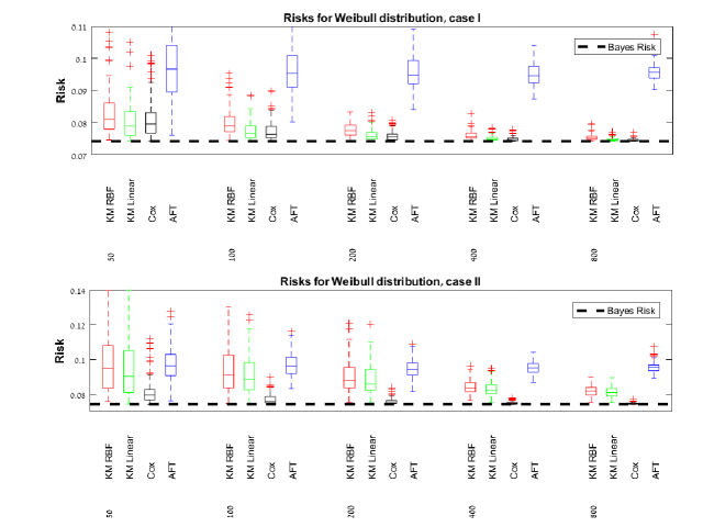
Figure 1: Weibull failure time distribution. The Bayes risk is the dashed line and the boxplots of the following risks are compared: KM-CSD with an RBF kernel, KM-CSD with a linear kernel, Cox, and AFT, for sample sizes $n=50,100,200,400,800$.

In Setting 2 (Multi-Weibull failure-time), the covariates $Z$ are generated uniformly on $[0,1]^{10},$ and the censoring variable $C$ is generated uniformly on $[0,\tau]$, as in setting 1. The failure time $T$ is generated from a Weibull distribution with parameters $scale=-0.5Z_{1}+2Z_{2}-Z_{3},\,shape=2$. The failure time was then truncated at $\tau=2$. Note that this model depends only on the first three variables. In Figure 2, boxplots of risks are presented.

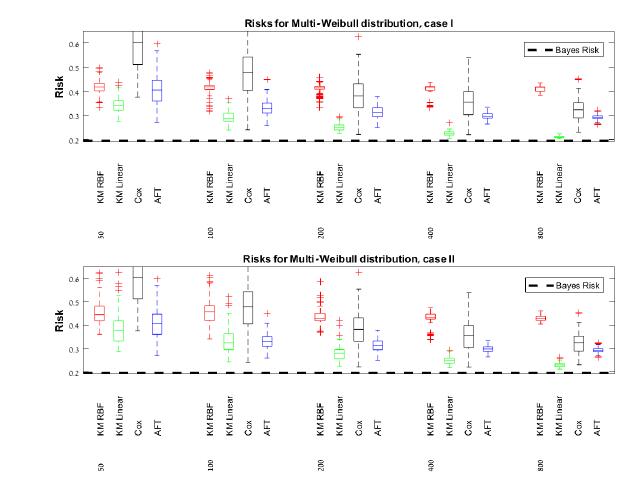
Figure 2: Multi-Weibull failure time distribution. The Bayes risk is the dashed line and the boxplots of the following risks are compared: the KM-CSD with an RBF kernel, the KM-CSD with a linear kernel, Cox, and AFT, for sample sizes $n=50,100,200,400,800$.

In Setting 3 (Multi-Log-Normal), the covariates $Z$ are generated uniformly on $[0,1]^{10},$ $C$ was generated as before and the failure time $T$ was generated from a Log-Normal distribution with parameters $\mu=\frac{1}{2}(0.3Z_{1}+0.5Z_{2}+0.2Z_{3}),\,\sigma=1$. The failure time was then truncated at $\tau=7$. Figure 3 presents the risks of the compared methods.

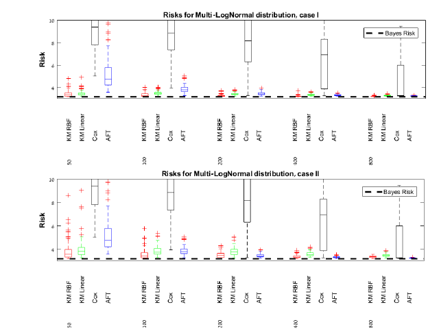
Figure 3: Multi-LogNormal failure time distribution. The Bayes risk is the dashed line and the boxplots of the following risks are compared: the KM-CSD with an RBF kernel, the KM-CSD with a linear kernel, Cox, and AFT, for sample sizes $n=50,100,200,400,800$.

In Setting 4, we considered a non-smooth conditional expectation function in the shape of a triangle. The covariates $Z$ are generated uniformly on $[0,1],$ $C$ is generated uniformly on $[0,\tau]$, and $T$ is generated according to the following

$$T=\begin{cases}4+6\cdot Z+\epsilon&,Z\leq 0.5\\ 10-6\cdot Z+\epsilon&,Z>0.5\end{cases},\,\,\mathrm{where}\,\,\epsilon\sim N(0,1).$$

The failure time was then truncated at $\tau=8$. In Figure 4, the boxplots of risks are presented.

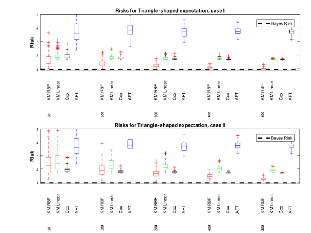
Figure 4: Triangle shaped failure time expectation. The Bayes risk is the dashed line and the boxplots of the following risks are compared: the KM-CSD with an RBF kernel, the KM-CSD with a linear kernel, Cox, and AFT, for sample sizes $n=50,100,200,400,800$.

To illustrate the flexibility of the KM-CSD, we also present a graphical representation of the true conditional expectation and its estimates, as a function of the covariates. Figure 5 compares the true expectation to the computed estimates for the case that $g$ is known; these estimates are based on the first iteration. As can be seen, the KM-CSD with an RBF kernel produces the most superior results.

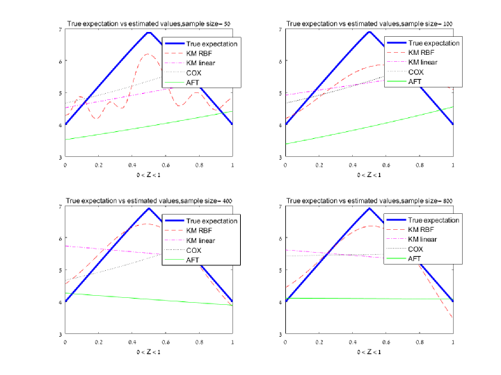
Figure 5: Triangle shaped failure time expectation, case I ($g$ is known). The true expectation is the thick triangle shaped line. The following estimates are compared: the KM-CSD with an RBF kernel, the KM-CSD with a linear kernel, Cox, and AFT, for sample sizes $n=50,100,400,800$.

To summarize, Figures 1-5 showed that the KM-CSD is comparable to other known methods for estimating the failure time distribution with current status data, and in certain cases is even better. Specifically, we found that the KM-CSD with an appropriate kernel was superior in three out of the four examples, especially when the true density $g$ is known. It should be noted that even when the assumptions of the other models were true, the KM-CSD estimates were comparable. Additionally, when these assumptions fail to hold, the KM-CSD estimates were generally better. The main advantage of the proposed kernel machines approach is that it does not assume any parametric form and thus may be superior, especially when the assumptions of other models fail to hold. Additionally, it seems that the KM-CSD can perform well in higher dimensions.

6 Real World Data Analysis

In this section we test our approach on two real-world data sets, and compare its performance to current state of the art. The first data set is current status data from immunological studies, and the second is real world data concerning news popularity, with artificial censoring. Note that the second data set was artificially censored by us, allowing us to train our method on current status data, and to test it on the true uncensored data. We used the mean squared error (MSE) in order to determine the best fit.

6.1 Current Status Data from Immunological Studies

We present an analysis of real world serological data on PVB19 and VZV infections. Both PVB19 and VZV cause a variety of diseases that mainly occur in childhood. The data was collected in Belgium between 2001 and 2003, as described in Hens et al. (2012). Blood samples were tested for presence of infection-specific IgG antibodies, reflecting infection experience. In addition, age at the time of data collection was registered. These blood samples are classified as either being seropositive or seronegative, based on some cut-off level, thus yielding current status data, with patient age being the monitoring time. The statistical analysis included in this paper is based on serological data on 2382 subjects with known immunological status for both PVB19 and VZV.

For our analysis, we use the patient’s age at the time of data collection as the monitoring time ($C$). We consider the continuous IgG antibody level of B19 as a covariate ($Z$) explaining the presence of the current status indicator VZV ($\Delta$). Note that we are treating the IgG antibody level of B19 as a baseline covariate, since we only have a single measurement of this antibody level. Also note that Hens et al. (2008) and Abrams and Hens (2015) have investigated the association between VZV and B19, and have shown that they share the same transmission route. Hence, there is a scientific justification for using the continuous IgG antibody level of B19 as a covariate explaining the presence of VZV.

We test our proposed KM-CSD on this data and compare it to estimates obtained by the Cox model and the AFT model. For the kernel of the RKHS $\mathcal{H}$, we used both a linear kernel and a Gaussian RBF kernel, where the kernel width $\sigma$ and the regularization parameter $\lambda$ were chosen using 5-fold cross-validation. It should be noted that we first standardized the covariates $Z$ (PVB19 antibody level) in order to suggest a reasonable selection of kernel widths. As before, the density of the censoring variable was estimated using nonparametric kernel density estimation with a normal kernel. In Figure 6, we present the results of the estimated expectation of time-to-infection of VZV, as a function of the covariates, for all four methods: KM with an RBF kernel, KM with a linear kernel, Cox, and AFT. It should be noted that since we do not know the true time-to-infection, we cannot argue that any model is superior. All four methods agree that there is a decreasing linear connection between time to infection of VZV, and B19 antibody level. In other words, the higher the level of PVB19, the lower the age of infection with VZV. This outcome supports previous research on joint transmission routes of VZV and B19. Further serological research can be done in order to better understand this relationship.

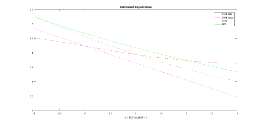
Figure 6: Conditional expectation of time to infection of VZV as a function of the standardized antibody level of B19. The following estimates are compared: the KM-CSD with an RBF kernel, the KM-CSD with a linear kernel, Cox and AFT.

6.2 Artificially Censored Real-World Data

For our second analysis, we used real-world data on news popularity, with artificial censoring. The original data summarizes a set of features regarding articles published by Mashable, in a period of two years, as described in Fernandes et al. (2015). The goal is to predict the number of shares of an article in social networks, referred to as ‘popularity’. Since the number of shares is non-negative, we consider it as our failure-time $T$. The original dataset contains 58 predictive attributes. As before, we first standardized the covariates $Z$. In order to reduce the dimensionality of the data, we used the LASSO method for subset selection (Tibshirani, 1996). For the sake of our analysis, we used the six most important explanatory variables. In order to obtain current status data, we generated the monitoring times $C_{1},...,C_{n}$ as random exponential variables with mean equal to the mean number of shares. We then calculated the current status indicator by $\Delta=\bm{1}_{\{T<C\}}$. In summary, the artificially censored data consists of six covariates, the current status indicator, and the monitoring time generated from an exponential distribution. The uncensored data after standardization and dimensionality reduction, and its artificially censored version, can be found in the Supplementary Materials.

Since the original dataset contains 39,644 entries, we divided it randomly into 35 training sets of 1000 observations, and one testing set of 4644 observations. The training sets consisted of the artificially censored data, whereas the testing data contained the original uncensored scaled number of shares. We trained the KM-CSD, with both a linear and a Gaussian RBF kernel, as well as Cox and AFT, on each training set. As before, the kernel width $\sigma$ and the regularization parameter $\lambda$ were chosen using 5-fold cross-validation. For a fair comparison, we estimated the density of the censoring variable using nonparametric kernel density estimation with a normal kernel, and did not use our knowledge regarding the censoring mechanism. For each training set, we computed the model predictions on the testing set and calculated the corresponding MSE. Since the MSE is sensitive to the overall scale of the response variable, we divided the MSE by the empirical variance of the number of shares in order to achieve standardized MSE. Figure 7 presents the boxplot of the standardized MSEs (SMSEs), for all four methods: KM-CSD with an RBF kernel, KM-CSD with a linear kernel, Cox, and AFT. Figure 7 shows that the SMSEs produced by the KM-CSD, with either a linear or a Gaussian kernel, is similar to the SMSEs produced by the Cox model, and is significantly lower than the SMSEs produced by the AFT model. In fact, the KM-CSD with a linear kernel produced the lowest SMSEs, whereas the KM-CSD with a Gaussian RBF kernel produced the SMSEs with the lowest variance. Additionally, for better readability of the results, we split the results into two sub-figures since the AFT produced much larger SMSEs than the other methods. It should also be noted that for some training sets, the AFT SMSE was so high that we had to omit it from the graphical representation.

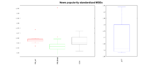
Figure 7: SMSEs of predicted number of shares, based on 35 training sets. The following estimates are compared: the KM-CSD with an RBF kernel, the KM-CSD with a linear kernel, Cox, and AFT. Note the different scale between the left and right subplots.

7 Concluding Remarks

We proposed a kernel-machine approach for estimation of the failure time expectation, studied its theoretical properties, presented a simulation study, and tested our approach on two real-world data sets. Specifically, we proved that our method is consistent, and showed by simulations and analysis of real-world data that our approach is just as good as current state of the art, and sometimes even better. We believe this work demonstrates an important approach in applying machine learning techniques to current status data. However, many open questions remain and many possible generalizations exist. First, note that we only studied the problem of estimating the failure time expectation and not other distribution related quantities. Further work needs to be done in order to extend the kernel machines approach to other estimation problems with current status data, and is beyond the scope of this paper. Note that the theory developed here might not hold in such generalizations, as the corresponding modified loss function will no longer be a convex function. Second, we assumed that the censoring is independent of the failure time given the covariates and that the censoring density is positive given the covariates over the entire observed time range. It would be worthwhile to study the consequences of violation of some of these assumptions. Third, it could be interesting to extend this work to other censored data formats such as interval censoring. We believe that further development and generalization of kernel machine learning methods for different types of censored data is of great interest. Some additional generalization of this work can include derivation of doubly-robust estimators and inclusion of time-dependent covariates. For the case of time-dependent covariates, one first needs to define an RKHS over the covariate process space and then to define the appropriate empirical risk minimization. Since this space is rich, the covering number results discussed in Section 4 may not hold for this space.

Supplementary Materials

The appendices referenced in Sections 3 and 4, the Matlab code for the algorithm, simulations, and data-analysis, and the artificially censored data used in Section 6.2, are available with this article.

Matlab code

Folder ‘SVR for CSD’ containing the Matlab code for both the algorithm and for the simulations. Please read the README.pdf for details on the files in this folder. A link to the folder can be found here.

Artificially censored data set

The data and the code for the data analysis in Section 6.2. This includes the uncensored data after standardization and dimensionality reduction and its artificially censored version, and the code that performs the analysis and produces Figure 7. Both data sets are Matlab .mat files, and the data analysis code is a Matlab .m file. The code is based on the functions defined in the folder ‘SVR for CSD’ described above.

Conflict of interest

The authors declare that they have no conflict of interest.

Appendix

A Computation of the Decision Function

Equation 1 is a quadratic optimization problem. Such problems are vastly studied in the literature (see, for example, Suykens and Vandewalle 1999) and known solutions exist. Specifically, using the representer theorem (Steinwart and Christmann 2008, Theorem 5.5), the solution of Equation 1 is given by

$$f_{D,\lambda}(Z)=\sum_{i=1}^{n}\alpha_{i}k(Z,Z_{i})+b.$$

Using the Lagrange method, the quadratic optimization problem in Eq. 1 can be simplified to a set of linear equations (see, for example, Fletcher 1987). Hence, it can be shown that the coefficients $\alpha_{1},...,\alpha_{n}$ and $b$ in the representation of $f_{D,\lambda}$ above can be obtained by

$$\left(\begin{array}[]{c}\alpha_{1}\\ \alpha_{2}\\ .\\ .\\ .\\ \alpha_{n}\\ b\end{array}\right)=\left(\begin{array}[]{ccccccc}K_{11}+n\lambda&K_{12}&.&.&.&K_{1n}&1\\ K_{21}&K_{22}+n\lambda&.&.&.&K_{2n}&1\\ .&.&.&&&.&.\\ .&.&&.&&.&.\\ .&.&&&.&.&.\\ K_{n1}&K_{n2}&.&.&.&K_{nn}+n\lambda&1\\ 1&1&.&.&.&1&0\end{array}\right)^{-1}.\left(\begin{array}[]{c}v_{1}\\ v_{2}\\ .\\ .\\ .\\ v_{n}\\ 0\end{array}\right),$$

where $\mathbf{K}_{n\times n}$ is the kernel matrix with entries $\mathbf{K}_{ij}=k(Z_{i},Z_{j})$, and where $v_{i}=(1-\Delta_{i})/g(C_{i}|Z_{i})$, for $1\leq i,j\leq n$. That is, the KM-CSD decision function has a closed form.

B Non-negative new modified loss function

Recall that our proposed loss function is

$$L^{n}(D,(Z,C,\Delta,s))=\frac{(1-\Delta)2(C-s)}{g(C|Z)}+s^{2}\,.$$

Note that this function is convex but not necessarily a loss function since it can obtain negative values. In order to ensure positivity we add a constant term that does not depend on $f$, and so our loss becomes

$$\widetilde{L^{n}}(D,(Z,C,\Delta,f(Z)))=\frac{(1-\Delta)2(C-f(Z))}{g(C|Z)}+\left(f(Z)\right)^{2}+a,$$

where for a fixed dataset of length $n,$ the constant $a$ is $a=\underset{1\leq i\leq n}{\max}\left\{(1-\Delta_{i})/\left(g(C_{i}|Z_{i})\right)^{2}\right\}.$ Note that this additional term will not effect the optimization (since $\widetilde{L^{n}}$ is just a shift by a constant of $L^{n}$) and thus will be neglected hereafter.

C Proofs

C.1 Proof of Theorem 1

Proof.

Since $L^{n}(D,(Z,C,\Delta,s))=\tau^{-2}\left((1-\Delta)2(C-s)/g(C|Z)+s^{2}\right)$ is convex, it implies that there exists a unique decision function (see Steinwart and Christmann, 2008, Section 5.1). For all distributions $Q$ on $\mathcal{Z\times Y}$, we define the kernel machine decision function by $f_{Q,\lambda}=\underset{f\in\mathcal{H}}{\inf}\lambda\left\|f\right\|_{\mathcal{H}}^{2}+R_{L,Q}(f).$ We note that for an RKHS $\mathcal{H}$ of a continuous kernel $k$ with $\left\|k\right\|_{\infty}\leq 1$,

$$\left\|f_{Q,\lambda}\right\|_{\mathcal{\infty}}\leq\left\|k\right\|_{\infty}\left\|f_{Q,\lambda}\right\|_{\mathcal{H}}\leq\left\|f_{Q,\lambda}\right\|_{\mathcal{H}}.$$

Hence,

$$\lambda\left\|f_{Q,\lambda}\right\|_{\mathcal{H}}^{2}\leq\lambda\left\|f_{Q,\lambda}\right\|_{\mathcal{H}}^{2}+R_{L,Q}(f_{Q,\lambda})=\underset{f\in\mathcal{H}}{\inf}\lambda\left\|f\right\|_{\mathcal{H}}^{2}+R_{L,Q}(f)\leq\lambda\left\|0\right\|_{\mathcal{H}}^{2}+R_{L,Q}(0)=R_{L,Q}(0),$$

Hence $\left\|f_{Q,\lambda}\right\|_{\mathcal{\infty}}\leq\left\|f_{Q,\lambda}\right\|_{\mathcal{H}}\leq\lambda^{-\nicefrac{{1}}{{2}}}\sqrt{R_{L,Q}(0)}$ for all $f\in\mathcal{H}$. By Remark 1, $L(y,0)\leq 1$ for all $y\in\mathcal{Y}$ and so we conclude that $R_{L,Q}(0)\leq 1$ and thus $\left\|f_{Q,\lambda}\right\|_{\mathcal{\infty}}\leq\left\|f_{Q,\lambda}\right\|_{\mathcal{H}}\leq\lambda^{-\nicefrac{{1}}{{2}}}$ for all distributions $Q$ on $\mathcal{Z\times Y}$.

Recall that the unit ball of $\mathcal{H}$ is denoted by $B_{H}$ and its closure by $\overline{B_{H}}$; since$\left\|f_{P,\lambda}\right\|_{\mathcal{H}}\leq\lambda^{-\nicefrac{{1}}{{2}}}$ we can write $f\in\lambda^{-\nicefrac{{1}}{{2}}}\overline{B_{H}}$. Since $\mathcal{Z}\subset\mathbb{\mathbb{R}}^{d}$ is compact, it implies that the $\left\|\cdot\right\|_{\infty}-\mathrm{closure}$ $\overline{B_{H}}$ of the unit ball $B_{H}$ is compact in $\ell_{\infty}(\mathcal{Z})$ (see Steinwart and Christmann, 2008, Corollary 4.31).

Denote by $R_{L^{n},D}(f)$ the empirical risk with respect to the data-dependent loss $L^{n}$. Since $f_{D,\lambda}$ minimizes $\lambda\left\|f\right\|_{\mathcal{H}}^{2}+R_{L^{n},D}(f)$,

$$\lambda\left\|f_{D,\lambda}\right\|_{\mathcal{H}}^{2}+R_{L^{n},D}(f_{D,\lambda})\leq\lambda\left\|f_{P,\lambda}\right\|_{\mathcal{H}}^{2}+R_{L^{n},D}(f_{P,\lambda}).$$

Recall that the approximation error is defined by $A_{2}(\lambda)=\underset{f\in\mathcal{H}}{\inf}\lambda\left\|f\right\|_{\mathcal{H}}^{2}+R_{L,P}(f)-R_{L,P}^{*}$, and thus, as in Steinwart and Christmann (2008, Eq. 6.18),

$$\lambda\left\|f_{D,\lambda}\right\|_{\mathcal{H}}^{2}+R_{L,P}(f_{D,\lambda})-R_{L,P}^{*}-A_{2}(\lambda)$$

$$= \lambda\left\|f_{D,\lambda}\right\|_{\mathcal{H}}^{2}+R_{L,P}(f_{D,\lambda})-\lambda\left\|f_{P,\lambda}\right\|_{\mathcal{H}}^{2}-R_{L,P}(f_{P,\lambda})$$

$$= \lambda\left\|f_{D,\lambda}\right\|_{\mathcal{H}}^{2}+R_{L^{n},D}(f_{D,\lambda})-R_{L^{n},D}(f_{D,\lambda})+R_{L,P}(f_{D,\lambda})-\lambda\left\|f_{P,\lambda}\right\|_{\mathcal{H}}^{2}-R_{L,P}(f_{P,\lambda})$$

$$\leq \lambda\left\|f_{P,\lambda}\right\|_{\mathcal{H}}^{2}+R_{L^{n},D}(f_{P,\lambda})-R_{L^{n},D}(f_{D,\lambda})+R_{L,P}(f_{D,\lambda})-\lambda\left\|f_{P,\lambda}\right\|_{\mathcal{H}}^{2}-R_{L,P}(f_{P,\lambda})$$

$$= R_{L^{n},D}(f_{P,\lambda})-R_{L^{n},D}(f_{D,\lambda})+R_{L,P}(f_{D,\lambda})-R_{L,P}(f_{P,\lambda})$$

$$\leq 2\underset{\left\|f\right\|_{\mathcal{H}}\leq\lambda^{-\nicefrac{{1}}{{2}}}}{\sup}|R_{L,P}(f)-R_{L^{n},D}(f)|.$$

That is,

$$\lambda\left\|f_{D,\lambda}\right\|_{\mathcal{H}}^{2}+R_{L,P}(f_{D,\lambda})-R_{L,P}^{*}-A_{2}(\lambda)\leq 2\underset{\left\|f\right\|_{\mathcal{H}}\leq\lambda^{-\nicefrac{{1}}{{2}}}}{\mathcal{\sup}}|R_{L,P}(f)-R_{L^{n},D}(f)|$$ (3)

Note that since $L$ is Lipschitz continuous, $|L(y,s)-L(y,s^{\prime})|\leq c_{L}|s-s^{\prime}|$ for all $s,s^{\prime}\in S$.

From the discussion above, we are only interested in bounded functions $f\in\lambda^{-\nicefrac{{1}}{{2}}}\overline{B_{H}}.$

Then for all $f\in\lambda^{-\nicefrac{{1}}{{2}}}\overline{B_{H}}$ we have

$$|L(y,f(z))|\text{$\leq$}|L(y,f(z))-L(y,0)|+L(y,0)\leq c_{L}|f(z)|+1\leq c_{L}\lambda^{-\nicefrac{{1}}{{2}}}+1\equiv B_{2}$$

thus we obtain that for functions $f\in\lambda^{-\nicefrac{{1}}{{2}}}\overline{B_{H}}$, the loss $L(y,f(z))$ is bounded.

For any $\epsilon>0,$ let $\mathcal{F_{\epsilon}}$ be an $\varepsilon-net$ of $\lambda^{-\nicefrac{{1}}{{2}}}\overline{B_{H}}$. Since $\overline{B_{H}}$ is compact, then the cardinality of the $\varepsilon-net$ is

$$|\mathcal{F}\varepsilon|=N\left(\lambda^{-\nicefrac{{1}}{{2}}}B_{H},\left\|\cdot\right\|_{\infty},\epsilon\right)=N(B_{H},\left\|\cdot\right\|_{\infty},\sqrt{\lambda}\epsilon)<\infty.$$

Thus for every $f\in\lambda^{-\nicefrac{{1}}{{2}}}\overline{B_{H}}$, there exists a function $h\in\mathcal{F_{\varepsilon}}$ with $\left\|f-h\right\|\leq\varepsilon$, and thus

$$|R_{L,P}(f)-R_{L^{n},D}(f)|$$ (4)

$$\leq|R_{L,P}(f)-R_{L,P}(h)|+|R_{L,P}(h)-R_{L^{n},D}(h)|+|R_{L^{n},D}(h)-R_{L^{n},D}(f)|$$

$$\equiv A_{n}+B_{n}+C_{n}$$

First we will bound $C_{n}$;

$$C_{n}\equiv \left|R_{L^{n},D}(h)-R_{L^{n},D}(f)\right|$$

$$\leq \left|\frac{1}{n}\sum_{i=1}^{n}\left[\frac{(1-\Delta_{i})\ell(C_{i},h(Z_{i}))}{g(C_{i}|Z_{i})}\right]-\frac{1}{n}\sum_{i=1}^{n}\left[\frac{(1-\Delta_{i})\ell(C_{i},f(Z_{i}))}{g(C_{i}|Z_{i})}\right]\right|$$

$$+ \left|\frac{1}{n}\sum_{i=1}^{n}[L(0,h(Z_{i}))]-\frac{1}{n}\sum_{i=1}^{n}[L(0,f(Z_{i}))]\right|$$

$$\equiv C_{n,1}+C_{n,2},$$

where

$$C_{n,1}\equiv \left|\frac{1}{n}\sum_{i=1}^{n}\left[\frac{(1-\Delta_{i})\ell(C_{i},h(Z_{i}))}{g(C_{i}|Z_{i})}-\frac{(1-\Delta_{i})\ell(C_{i},f(Z_{i}))}{g(C_{i}|Z_{i})}\right]\right|$$

$$= \left|\frac{1}{n}\sum_{i=1}^{n}\left[\frac{(1-\Delta_{i})}{g(C_{i}|Z_{i})}\left(\ell(C_{i},h(Z_{i}))-\ell(C_{i},f(Z_{i}))\right)\right]\right|$$

$$\leq \left|\frac{1}{n}\sum_{i=1}^{n}\left[\frac{1}{g(C_{i}|Z_{i})}\left(\ell(C_{i},h(Z_{i}))-\ell(C_{i},f(Z_{i}))\right)\right]\right|$$

$$\leq \frac{1}{2\kappa}\left|\frac{1}{n}\sum_{i=1}^{n}\left[\ell(C_{i},h(Z_{i}))-\ell(C_{i},f(Z_{i}))\right]\right|\leq\frac{1}{2n\kappa}\sum_{i=1}^{n}|\ell(C_{i},h(Z_{i}))-\ell(C_{i},f(Z_{i}))|$$

$$\leq \frac{1}{2n\kappa}\sum_{i=1}^{n}c_{l}|h(Z_{i})-f(Z_{i})|\leq\frac{1}{2n\kappa}\sum_{i=1}^{n}c_{l}\varepsilon=\frac{c_{l}\varepsilon}{2\kappa},$$

and where

$$C_{n,2}\equiv \left|\frac{1}{n}\sum_{i=1}^{n}[L(0,h(Z_{i}))-L(0,f(Z_{i}))]\right|$$

$$\leq \frac{1}{n}\sum_{i=1}^{n}\left|L(0,h(Z_{i}))-L(0,f(Z_{i}))\right|$$

$$\leq \frac{1}{n}\sum_{i=1}^{n}c_{L}|h(Z_{i})-f(Z_{i})|\leq\frac{1}{n}\sum_{i=1}^{n}\left[c_{L}\varepsilon\right]=c_{L}\varepsilon$$

So we were able to bound $C_{n}$ by $c_{l}\varepsilon/2\kappa+c_{L}\varepsilon$.

Similarly, using to the property that $E\left[\alpha\right]=\alpha$ for any constant $\alpha$, it can be shown that $A_{n}\leq c_{l}\varepsilon/2\kappa+c_{L}\varepsilon$.

As an interim summary, we showed that

$$\underset{f\in\lambda^{-\nicefrac{{1}}{{2}}}B_{H}}{\sup}|R_{L,P}(f)-R_{L^{n},D}(f)|\leq\underset{h\in\mathcal{F_{\varepsilon}}}{\sup}\underset{=B_{n}}{\underbrace{|R_{L,P}(h)-R_{L^{n},D}(h)|}}+\frac{1}{\kappa}c_{l}\varepsilon+2c_{L}\varepsilon.$$ (5)

Recall that the loss $L(y,f(z))$ is bounded by $B_{2}$ and that by Remark 1, $\ell(y,s)\leq B_{1}$.

We note that

$$\frac{(1-\Delta)\ell(C,h(Z))}{g(C|Z)}+L(0,h(Z)) \leq\frac{\ell(C,h(Z))}{g(C|Z)}+L(0,h(Z))\leq \frac{B_{1}}{2\kappa}+B_{2}\equiv B$$

Combining this with equation (3), we obtain that

$$Pr \left(\lambda\left\|f_{D,\lambda}\right\|_{\mathcal{H}}^{2}+R_{L,P}(f_{D,\lambda})-R_{L,P}^{*}-A_{2}(\lambda)\geq B\sqrt{\frac{2\eta}{n}}+\frac{2c_{l}\varepsilon}{\kappa}+4c_{L}\varepsilon\right)$$

$$\leq Pr\left(2\underset{\left\|f\right\|_{\mathcal{H}}\leq\lambda^{-\nicefrac{{1}}{{2}}}}{sup}|R_{L,P}(f)-R_{L^{n},D}(f)|\geq B\sqrt{\frac{2\eta}{n}}+\frac{2c_{l}\varepsilon}{\kappa}+4c_{L}\varepsilon\right) \,(\mathrm{by\,eq.\,}\ref{eq:first bound})$$

$$\leq Pr\left(2\left(\underset{h\in\mathcal{F_{\varepsilon}}}{sup}|R_{L,P}(h)-R_{L^{n},D}(h)|+\frac{1}{\kappa}c_{l}\varepsilon+2c_{L}\varepsilon\right)\geq B\sqrt{\frac{2\eta}{n}}+\frac{2c_{l}\varepsilon}{\kappa}+4c_{L}\varepsilon\right) \,(\mathrm{by\,eq.\,}\ref{eq:second bound})$$

$$= Pr\left(2\left(\underset{h\in\mathcal{F_{\varepsilon}}}{\sup}B_{n}+\frac{1}{\kappa}c_{l}\varepsilon+2c_{L}\varepsilon\right)\geq B\sqrt{\frac{2\eta}{n}}+\frac{2c_{l}\varepsilon}{\kappa}+4c_{L}\varepsilon\right)$$

$$= Pr\left(\underset{h\in\mathcal{F_{\varepsilon}}}{\sup}B_{n}\geq B\sqrt{\frac{\eta}{2n}}\right)=Pr\left(\underset{h\in\mathcal{F_{\varepsilon}}}{\sup}\left|R_{L,P}(h)-R_{L^{n},D}(h)\right|\geq B\sqrt{\frac{\eta}{2n}}\right).$$

By the union bound, the last expression is bounded by

$$\underset{h\in\mathcal{F_{\varepsilon}}}{\sum}Pr\left(|R_{L,P}(h)-R_{L^{n},D}(h)|\geq B\sqrt{\frac{\eta}{2n}}\right),$$

which can then be bounded again by $2|\mathcal{F}_{\varepsilon}|\exp(-\eta)$, using Hoeffding’s inequality (Steinwart and Christmann, 2008, Theorem 6.10); where $\mathcal{F_{\epsilon}}$ is an $\varepsilon$-net of $\lambda^{-\nicefrac{{1}}{{2}}}\overline{B_{H}}$ with cardinality

$$|\mathcal{F}\varepsilon|=N\left(\lambda^{-\nicefrac{{1}}{{2}}}B_{H},\left\|\cdot\right\|_{\infty},\epsilon\right)<\infty.$$

Define $\eta=\log(2|\mathcal{F_{\varepsilon}}|)+\theta$, then

$$Pr\left(\lambda\left\|f_{D,\lambda}\right\|_{\mathcal{H}}^{2}+R_{L,P}(f_{D,\lambda})-R_{L,P}^{*}-A_{2}(\lambda)\geq B\sqrt{\frac{2(\log(2|\mathcal{F_{\varepsilon}}|)+\theta)}{n}}+\frac{2c_{l}\varepsilon}{\kappa}+4c_{L}\varepsilon\right)$$

$$\leq\exp(-\theta),$$

which concludes the proof. ∎

C.2 Proof of Corollary 1

Proof.

In Theorem 1 we showed that

$$\lambda\left\|f_{D,\lambda}\right\|_{\mathcal{H}}^{2}+R_{L,P}(f_{D,\lambda})-R_{L,P}^{*}-A_{2}(\lambda)\leq B\sqrt{\frac{2\log\left(2N(\sqrt{\frac{1}{\lambda}}B_{H},\left\|\cdot\right\|_{\infty},\epsilon)\right)+2\theta}{n}}+\frac{2c_{l}\varepsilon}{\kappa}+4c_{L}\varepsilon,$$

with probability not less than $1-\exp^{-\theta}$.

Choose $\lambda=\lambda_{n};$ from Assumption (A5) together with Lemma 5.15 of Steinwart and Christmann (2008, 5.15), $A_{2}(\lambda_{n})$ converges to zero as $n$ goes to infinity. By the assumption $\log\left(N(B_{H},\left\|\cdot\right\|_{\infty},\epsilon)\right)\leq a\epsilon^{-2p}$, we have that

$$\log\left(2N(B_{H},\left\|\cdot\right\|_{\infty},\sqrt{\lambda}\epsilon)\right)$$

$$=\log(2)+\log\left(N(B_{H},\left\|\cdot\right\|_{\infty},\sqrt{\lambda}\epsilon)\right)$$

$$\leq\log(2)+a\left(\sqrt{\lambda}\epsilon\right)^{-2p}$$

$$\leq 1+a\left(\sqrt{\lambda}\epsilon\right)^{-2p}.$$

Choose $\epsilon=\left(\frac{p}{2}\right)^{\frac{1}{1+p}}\left(\frac{2a}{n}\right)^{\frac{1}{2+2p}}\frac{1}{\sqrt{\lambda}}$ and recall that $a\geq 1$. Then for $n\geq\frac{p^{2}a}{2}$ we have

$$\log\left(2N(B_{H},\left\|\cdot\right\|_{\infty},\sqrt{\lambda}\epsilon)\right)$$

$$\leq 1+a\left(\sqrt{\lambda}\epsilon\right)^{-2p}$$

$$=1+a\left(\left(\frac{p}{2}\right)^{\frac{1}{1+p}}\left(\frac{2a}{n}\right)^{\frac{1}{2+2p}}\right)^{-2p}$$

$$\leq 2a\left(\left(\frac{p}{2}\right)^{\frac{1}{1+p}}\left(\frac{2a}{n}\right)^{\frac{1}{2+2p}}\right)^{-2p}$$

.

Recall that $B$ is defined by $B=\frac{B_{1}}{2\kappa}+c_{L}\lambda^{-\frac{1}{2}}+1$. Hence, from the assumption on the covering number we have that

$$B\sqrt{\frac{2\log\left(2N(\sqrt{\frac{1}{\lambda}}B_{H},\left\|\cdot\right\|_{\infty},\epsilon)\right)+2\theta}{n}}\leq\left(\frac{B_{1}}{2\kappa}+c_{L}\lambda^{-\frac{1}{2}}+1\right)\sqrt{\frac{4a\left(\left(\frac{p}{2}\right)^{\frac{1}{1+p}}\left(\frac{2a}{n}\right)^{\frac{1}{2+2p}}\right)^{-2p}+2\theta}{n}}$$

and since $\lambda_{n}^{1+p}n\underset{n\rightarrow\infty}{\rightarrow}\infty$, the right hand side of this converges to 0 as $n\rightarrow\infty$. Finally, from the choice of $\epsilon$, it follows that both $\frac{2c_{l}\varepsilon}{\kappa}$ and $4c_{L}\varepsilon$ converge to 0 as $n\rightarrow\infty$. Hence for every fixed $\theta,$

$$\lambda_{n}\left\|f_{D,\lambda_{n}}\right\|_{\mathcal{H}}^{2}+R_{L,P}(f_{D,\lambda_{n}})-R_{L,P}^{*}\leq A_{2}(\lambda_{n})+B\sqrt{\frac{2\log\left(2N(\sqrt{\frac{1}{\lambda_{n}}}B_{H},\left\|\cdot\right\|_{\infty},\epsilon)\right)+2\theta}{n}}+\frac{2c_{l}\varepsilon}{\kappa}+4c_{L}\varepsilon$$

with probability not less than $1-\exp(-\theta)$. The right hand side of this converges to 0 as $n\rightarrow\infty$, which implies consistency (Steinwart and Christmann, 2008, Lemma 6.5). Since this holds for all probability measures $P\in\mathcal{P}$, we obtain $\mathcal{P}$-universal consistency. ∎

C.3 Proof of Lemma 1

Proof.

For the sake of completeness, we develop here a finite sample bound on the difference between the kernel density estimator $\hat{g}$ and the true density $g$. While asymptotic results for kernel density estimators are well known in the literature (see, for example, Silverman 1978), finite sample bounds were not previously studied. In order to develop our bound, we incorporate Bernstein’s inequality in our analysis as described below.

Note that

$$\frac{1}{n}\sum_{i=1}^{n}\left|\hat{g}(C_{i})-g(C_{i})\right|\leq$$

$$\leq \frac{1}{n}\sum_{i=1}^{n}\left|\hat{g}(C_{i})-E\left[\hat{g}(C_{i})\right]\right|+\frac{1}{n}\sum_{i=1}^{n}\left|E\left[\hat{g}(C_{i})\right]-g(C_{i})\right|\equiv A+B$$

As in Tsybakov (2008, Proposition 1.1), for any $c_{0}\in\mathcal{Y}$, define

$$\eta_{i}(c_{0})=K_{m}\left(\frac{C_{i}-c_{0}}{h}\right)-E_{g}\left[K_{m}\left(\frac{C_{i}-c_{0}}{h}\right)\right].$$

Then $\eta_{i}(c_{0})$, for $i=1,...,n$ are i.i.d. random variables with zero mean and with variance:

$$\mathrm{Var}\left[\eta_{i}(c_{0})\right] =E_{g}\left[\left(\eta_{i}(c_{0})\right)^{2}\right]=E_{g}\left[\left(K_{m}\left(\frac{C_{i}-c_{0}}{h}\right)-E_{g}\left[K_{m}\left(\frac{C_{i}-c_{0}}{h}\right)\right]\right)^{2}\right]\leq E_{g}\left[K_{m}^{2}\left(\frac{C_{i}-c_{0}}{h}\right)\right]$$

$$=\int_{u}{K_{m}^{2}\left(\frac{u-c_{0}}{h}\right)g(u)du}\leq g_{max}\int_{u}K_{m}^{2}\left(\frac{u-c_{0}}{h}\right)du\stackrel{{\scriptstyle}}{{=g_{max}h\int_{v}K_{m}^{2}\left(v\right)dv=D_{1}h}}$$

where the equality before last follows from change of variables and where $D_{1}=g_{max}\int_{v}K_{m}^{2}\left(v\right)dv$. Thus $\mathrm{Var}(\hat{g}(c_{0}))=E_{g}\left[\left(\frac{1}{nh}\sum_{i=1}^{n}\eta_{i}(c_{0})\right)^{2}\right]=\frac{1}{nh^{2}}E_{g}\left[\eta_{1}^{2}(c_{0})\right]\leq\frac{D_{1}h}{nh^{2}}=\frac{D_{1}}{nh}.$

Note that $\mathrm{Var}(\left|\hat{g}(c_{0})-E\left[\hat{g}(c_{0})\right|\right])=E\left[\left(\left|\hat{g}(c_{0})-E\left[\hat{g}(c_{0})\right]\right|\right)^{2}\right]=\mathrm{Var}(\hat{g}(c_{0})-E\left[\hat{g}(c_{0})\right])=\mathrm{Var}(\hat{g}(c_{0}))$. Hence $\mathrm{Var}(\left|\hat{g}(c_{0})-E\left[\hat{g}(c_{0})\right|\right])=\mathrm{Var}(\hat{g}(c_{0}))\leq\frac{D_{1}}{nh}$. Using Bernstein’s inequality, for any $\theta>0$ we have

$$Pr\left(A>\sqrt{\frac{2D_{1}\theta}{n^{2}h}}+\frac{2g_{max}\theta}{3n}\right)\equiv Pr\left(\frac{1}{n}\sum_{i=1}^{n}\left|\hat{g}(C_{i})-E\left[\hat{g}(C_{i})\right]\right|>\sqrt{\frac{2D_{1}\theta}{n^{2}h}}+\frac{2g_{max}\theta}{3n}\right)\leq\exp(-\theta)$$

For the second term, as in Tsybakov (2008, Proposition 1.2), we have that

$$B\equiv\frac{1}{n}\sum_{i=1}^{n}\left|E\left[\hat{g}(C_{i})\right]-g(C_{i})\right|\leq D_{2}h^{\beta}$$

where $D_{2}=\mathcal{L}\left|\pi\right|^{\beta-m}/m!\int_{-\infty}^{\infty}{\left|K_{m}\left(v\right)\right|}\left|v\right|^{\beta}dv<\infty$, and for some $\pi\in[0,1].$

In conclusion, we showed that

$$Pr\left(\frac{1}{n}\sum_{i=1}^{n}\left|\hat{g}(C_{i})-g(C_{i})\right|>\sqrt{\frac{2D_{1}\theta}{n^{2}h}}+\frac{2g_{max}\theta}{3n}+D_{2}\cdot h^{\beta}\right)$$

$$\leq Pr\left(\frac{1}{n}\sum_{i=1}^{n}\left|\hat{g}(C_{i})-E\left[\hat{g}(C_{i})\right]\right|+\frac{1}{n}\sum_{i=1}^{n}\left|E\left[\hat{g}(C_{i})\right]-g(C_{i})\right|>\sqrt{\frac{2D_{1}\theta}{n^{2}h}}+\frac{2g_{max}\theta}{3n}+D_{2}\cdot h^{\beta}\right)$$

$$\leq Pr\left(\frac{1}{n}\sum_{i=1}^{n}\left|\hat{g}(C_{i})-E\left[\hat{g}(C_{i})\right]\right|+D_{2}\cdot h^{\beta}>\sqrt{\frac{2D_{1}\theta}{n^{2}h}}+\frac{2g_{max}\theta}{3n}+D_{2}\cdot h^{\beta}\right)$$

$$= Pr\left(\frac{1}{n}\sum_{i=1}^{n}\left|\hat{g}(C_{i})-E\left[\hat{g}(C_{i})\right]\right|>\sqrt{\frac{2D_{1}\theta}{n^{2}h}}+\frac{2g_{max}\theta}{3n}\right)\leq\exp(-\theta)$$

where $h$ is the bandwidth. ∎

C.4 Proof of Theorem 2

Proof.

Note that the proof of this theorem is similar to the proof of of Theorem 1 and thus we will only discuss the parts of the proof where they differ. As in Theorem 1, equation 4,

$$\lambda\left\|f_{D,\lambda}\right\|_{\mathcal{H}}^{2}+R_{L,P}(f_{D,\lambda})-R_{L,P}^{*}-A_{2}(\lambda)\leq 2\left(A_{n}+B_{n}+C_{n}\right)$$

where

$$A_{n}\equiv|R_{L,P}(f)-R_{L,P}(v)|,\,\,B_{n}\equiv|R_{L,P}(v)-R_{L^{n},D}(v)|,\,\,\mathrm{and\,where}\,\,C_{n}\equiv|R_{L^{n},D}(v)-R_{L^{n},D}(f)|,$$

Since $A_{n}$ does not depend on the data-set $D,$ the same bound holds as in the proof of Theorem 1, that is, $A_{n}\leq c_{l}\varepsilon/2\kappa+c_{L}\varepsilon$.

We bound $C_{n}$ as follows:

$$C_{n}\equiv \left|R_{L^{n},D}(v)-R_{L^{n},D}(f)\right|$$

$$\leq \left|\frac{1}{n}\sum_{i=1}^{n}\left[\frac{(1-\Delta_{i})\ell(C_{i},v(Z_{i}))}{\hat{g}(C_{i})}\right]-\frac{1}{n}\sum_{i=1}^{n}\left[\frac{(1-\Delta_{i})\ell(C_{i},f(Z_{i}))}{\hat{g}(C_{i})}\right]\right|$$

$$+ \left|\frac{1}{n}\sum_{i=1}^{n}[L(0,v(Z_{i}))]-\frac{1}{n}\sum_{i=1}^{n}[L(0,f(Z_{i}))]\right|$$

$$\equiv C_{n,1}+C_{n,2}$$

Using the same arguments as in Theorem 1, we can bound $C_{n}$ by $c_{l}\varepsilon/\kappa+c_{L}\varepsilon$. Note that the only difference is in the denominator of $C_{n,1}$ since $g^{-1}\leq(2\kappa)^{-1}$ and $\hat{g}^{-1}\leq\kappa^{-1}$.

Recall that the loss $L(y,f(z))$ is bounded by $B_{2}$. Define $R_{L^{n},D,g}(v)$ by

$$R_{L^{n},D,g}(v)=\frac{1}{n}\sum_{i=1}^{n}\left[\frac{(1-\Delta_{i})\ell(C_{i},v(Z_{i}))}{g(C_{i})}\right]+\frac{1}{n}\sum_{i=1}^{n}[L(0,v(Z_{i}))].$$

In other words, $R_{L^{n},D,g}(v)$ is the empirical risk with the true censoring density function $g$.

We bound $B_{n}$ as follows

$$B_{n}= |R_{L,P}(v)-R_{L^{n},D}(v)|$$

$$\leq \left|R_{L,P}(v)-R_{L^{n},D,g}(v)\right|+\left|R_{L^{n},D,g}(v)-R_{L^{n},D}(v)\right|\equiv B_{n,1}+B_{n,2}$$

where

$$\frac{(1-\Delta)\ell(C,v(Z))}{g(C)}+L(0,v(Z)) \leq\frac{\ell(C,v(Z))}{g(C)}+L(0,v(Z))\leq \frac{B_{1}}{2\kappa}+B_{2}=B$$

and where

$$B_{n,2}= \left|R_{L^{n},D,g}(v)-R_{L^{n},D}(v)\right|=$$

$$= \left|\frac{1}{n}\sum_{i=1}^{n}\left[\frac{(1-\Delta_{i})\ell(C_{i},v(Z_{i}))}{g(C_{i})}\right]-\frac{1}{n}\sum_{i=1}^{n}\left[\frac{(1-\Delta_{i})\ell(C_{i},v(Z_{i}))}{\hat{g}(C_{i})}\right]\right|$$

$$= \left|\frac{1}{n}\sum_{i=1}^{n}\left[(1-\Delta_{i})\ell(C_{i},v(Z_{i}))\left(\frac{1}{g(C_{i})}-\frac{1}{\hat{g}(C_{i})}\right)\right]\right|$$

$$\leq \frac{1}{n}\sum_{i=1}^{n}\left[\left|\ell(C_{i},v(Z_{i}))\left(\frac{1}{g(C_{i})}-\frac{1}{\hat{g}(C_{i})}\right)\right|\right]$$

$$= \frac{B_{1}}{n}\sum_{i=1}^{n}\left[\left|\frac{\hat{g}(C_{i})-g(C_{i})}{g(C_{i})\hat{g}(C_{i})}\right|\right]\leq\frac{B_{1}}{2\kappa^{2}n}\sum_{i=1}^{n}\left[\left|\hat{g}(C_{i})-g(C_{i})\right|\right].$$

Note that these inequalities hold for all functions $v\in\mathcal{F_{\varepsilon}}\subseteq\lambda^{-\nicefrac{{1}}{{2}}}B_{H}$. We would like to bound the last expression using Lemma 1. Let

$$\eta=\frac{B_{1}}{2\kappa^{2}}\left(\sqrt{\frac{2D_{1}\theta}{n^{2}h}}+\frac{2g_{max}\theta}{3n}+D_{2}\cdot h^{\beta}\right),$$

then by Lemma 1

$$Pr(B_{n,2}>\eta)\leq Pr\left(\frac{B_{1}}{2\kappa^{2}n}\sum_{i=1}^{n}\left[\left|\hat{g}(C_{i})-g(C_{i})\right|\right]>\eta\right)$$

$$= Pr\left(\frac{B_{1}}{2\kappa^{2}n}\sum_{i=1}^{n}\left[\left|\hat{g}(C_{i})-g(C_{i})\right|\right]>\frac{B_{1}}{2\kappa^{2}}\left(\sqrt{\frac{2D_{1}\theta}{n^{2}h}}+\frac{2g_{max}\theta}{3n}+D_{2}\cdot h^{\beta}\right)\right)$$

$$= Pr\left(\frac{1}{n}\sum_{i=1}^{n}\left[\left|\hat{g}(C_{i})-g(C_{i})\right|\right]>\left(\sqrt{\frac{2D_{1}\theta}{n^{2}h}}+\frac{2g_{max}\theta}{3n}+D_{2}\cdot h^{\beta}\right)\right)$$

$$\leq \exp(-\theta).$$

We need to bound the term $B_{n,1}(v)\equiv\left|R_{L,P}(v)-R_{L^{n},D,g}(v)\right|$. By the union bound, for all $\mu>0$

$$Pr\left(\underset{v\in\mathcal{F_{\varepsilon}}}{\sup}B_{n,1}(v)\geq B\sqrt{\frac{\mu}{2n}}\right) =Pr\left(\underset{v\in\mathcal{F_{\varepsilon}}}{\sup}\left|R_{L,P}(v)-R_{L^{n},D,g}(v)\right|\geq B\sqrt{\frac{\mu}{2n}}\right)$$

$$\leq\underset{v\in\mathcal{F_{\varepsilon}}}{\sum}Pr\left(|R_{L,P}(v)-R_{L^{n},D,g}(v)|\geq B\sqrt{\frac{\mu}{2n}}\right).$$

We showed that $(1-\Delta)\ell(C,v(Z))/g(C)+L(0,v(Z))\leq B$. Note also that $R_{L,P}(v)=R_{L^{n},P}(v)=R_{L^{n},P,g}(v)$; That is, $R_{L,P}(v)$ is the expectation of $R_{L^{n},D,g}(v)$. Hence by Hoeffding’s inequality, the last term can then be bounded again by $2|\mathcal{F}_{\varepsilon}|\exp(-\mu)$, where $\mathcal{F_{\epsilon}}$ is an $\varepsilon$-net of $\lambda^{-\nicefrac{{1}}{{2}}}\overline{B_{H}}$ with cardinality

$$|\mathcal{F}\varepsilon|=N\left(\lambda^{-\nicefrac{{1}}{{2}}}B_{H},\left\|\cdot\right\|_{\infty},\epsilon\right)<\infty.$$

Define $\mu=\log(2|\mathcal{F_{\varepsilon}}|)+\theta$, then

$$Pr\left(\underset{v\in\mathcal{F_{\varepsilon}}}{\sup}B_{n,1}(v)\geq B\sqrt{\frac{ln(2|\mathcal{F_{\varepsilon}}|)+\theta}{2n}}\right)\leq\exp(-\theta)$$

In conclusion we have that

$$Pr \left(\lambda\left\|f_{D,\lambda}\right\|_{\mathcal{H}}^{2}+R_{L,P}(f_{D,\lambda})-R_{L,P}^{*}-A_{2}(\lambda)\geq B\sqrt{\frac{2\mu}{n}}+\frac{3c_{l}\varepsilon}{\kappa}+4c_{L}\varepsilon+2\eta\right)$$

$$\leq Pr\left(2\underset{\left\|f\right\|_{\mathcal{H}}\leq\lambda^{-\nicefrac{{1}}{{2}}}}{sup}|R_{L,P}(f)-R_{L^{n},D}(f)|\geq B\sqrt{\frac{2\mu}{n}}+\frac{3c_{l}\varepsilon}{\kappa}+4c_{L}\varepsilon+2\eta\right)$$

$$\leq Pr\left(2\left(\underset{v\in\mathcal{F_{\varepsilon}}}{sup}|R_{L,P}(v)-R_{L^{n},D}(v)|+\frac{3}{2\kappa}c_{l}\varepsilon+2c_{L}\varepsilon\right)\geq B\sqrt{\frac{2\mu}{n}}+\frac{3c_{l}\varepsilon}{\kappa}+4c_{L}\varepsilon+2\eta\right)$$

$$\leq Pr\left(2\left(\underset{v\in\mathcal{F_{\varepsilon}}}{\sup}B_{n,1}(v)+B_{n,2}(v)\right)\geq B\sqrt{\frac{2\mu}{n}}+2\eta\right)$$

$$\leq Pr\left(\underset{v\in\mathcal{F_{\varepsilon}}}{\sup}B_{n,1}(v)+B_{n,2}(v)\geq B\sqrt{\frac{\mu}{2n}}+\eta\right)$$

$$\leq Pr\left(\underset{v\in\mathcal{F_{\varepsilon}}}{\sup}B_{n,1}\geq B\sqrt{\frac{ln(2|\mathcal{F_{\varepsilon}}|)+\theta}{2n}}\right)+Pr\left(\underset{v\in\mathcal{F_{\varepsilon}}}{\sup}B_{n,2}(v)\geq\eta\right)$$

$$\leq \exp(-\theta)+\exp(-\theta)=2\exp(-\theta)$$

and the result follows. ∎

C.5 Proof of Corollary 2

Proof.

Note that the only difference between Corollary 2 and Corollary 1 is in the term $2\eta$. Recall that $\eta$ is defined by $\eta\equiv\frac{B_{1}}{2\kappa^{2}}\left(\sqrt{\frac{2D_{1}\theta}{n^{2}h}}+\frac{2g_{max}\theta}{3n}+D_{2}\cdot h^{\beta}\right)$. Choose $h$ such that $h\underset{n\rightarrow\infty}{\rightarrow}0$ and that $h^{0.5}n\underset{n\rightarrow\infty}{\rightarrow}\infty$. Then $\eta\underset{n\rightarrow\infty}{\rightarrow}0$. Choose $\lambda=\lambda_{n}$ and $\epsilon=\left(\frac{p}{2}\right)^{\frac{1}{1+p}}\left(\frac{2a}{n}\right)^{\frac{1}{2+2p}}\frac{1}{\sqrt{\lambda}}$. Then as in Corollary 1, all other terms converge to zero as ${n\rightarrow\infty}$ which implies consistency (Steinwart and Christmann, 2008, Lemma 6.5). Since this holds for all probability measures $P\in\mathcal{P}$, we obtain $\mathcal{P}$-universal consistency. ∎

D Learning Rates

In this subsection we derive learning rates for cases I and II.

Definition 4.

A learning method is said to learn with rate $\epsilon_{n}\subset(0,1]$ that converges to zero if for all $n\geq 1$ and all $\tau\in(0,1]$, $Pr\left(R_{L,P}(f_{D})-R_{L,P}^{*}\leq c_{P}c_{\tau}\epsilon_{n}\right)\geq 1-\tau$ , where $c_{\tau}$ and $c_{P}$ are constants such that $c_{\tau}\in[1,\infty)$ and $c_{P}>0$.

We demonstrate how to derive learning rates from the same oracle inequalities used for the consistency proofs. While faster learning rates can be achieved under further assumptions in a similar manner, they further complicate the calculations and are beyond the scope of this paper.

Theorem 3.

Assume that (A1)-(A4) hold. Choose $0<\lambda_{n}<1$ and assume that there exist constants $a\geq 1,\,p>0$ such that $\log\left(N(B_{H},\left\|\cdot\right\|_{\infty},\epsilon)\right)\leq a\epsilon^{-2p}$. Additionally, assume that there exist constants $c>0,\,\gamma\in(0,1]$ such that $A_{2}(\lambda)\leq c\lambda^{\gamma}$. Then

(i) If $g$ is known, the learning rate is given by $n^{-\frac{\gamma}{(1+p)(2\gamma+1)}}$.

(ii) If $g$ is not known and the setup of Theorem 2 holds, then the leraning rate is given by $n^{-\min\left(\frac{\gamma}{(1+p)(2\gamma+1)},\frac{2\beta}{2\beta+1}\right)}$.

D.1 Proof of Theorem 3

Proof.

Case I

By Theorem 1,

$$\lambda\left\|f_{D,\lambda}\right\|_{\mathcal{H}}^{2}+R_{L,P}(f_{D,\lambda})-R_{L,P}^{*}-A_{2}(\lambda)\leq B\sqrt{\frac{2\log\left(2N(\lambda^{-\nicefrac{{1}}{{2}}}B_{H},\left\|\cdot\right\|_{\infty},\epsilon)\right)+2\theta}{n}}+\frac{2c_{l}\varepsilon}{\kappa}+4c_{L}\varepsilon$$

with probability not less than $1-\exp(-\theta)$. For any compact set $\mathcal{S}=[-S,S]\subset\mathbb{R}$, Both $L$ and $l$ are bounded and Lipschitz continuous with Lipschitz constants $c_{L}\leq 2\tau^{-2}(S+\tau)$ and $c_{l}=2\tau^{-2}$. Hence,

$$\lambda\left\|f_{D,\lambda}\right\|_{\mathcal{H}}^{2}+R_{L,P}(f_{D,\lambda})-R_{L,P}^{*}-A_{2}(\lambda)$$ (6)

$$\leq B\sqrt{\frac{2\log\left(2N(B_{H},\left\|\cdot\right\|_{\infty},\sqrt{\lambda}\epsilon)\right)+2\theta}{n}}+\frac{2c_{l}\varepsilon}{\kappa}+4c_{L}\varepsilon$$

$$\leq B\sqrt{\frac{2\log\left(2N(B_{H},\left\|\cdot\right\|_{\infty},\sqrt{\lambda}\epsilon)\right)+2\theta}{n}}+\frac{4\varepsilon}{\kappa\tau^{2}}+\frac{8(S+\tau)}{\tau^{2}}\varepsilon$$

$$= B\sqrt{\frac{2\log\left(2N(B_{H},\left\|\cdot\right\|_{\infty},\sqrt{\lambda}\epsilon)\right)+2\theta}{n}}+M\cdot\epsilon$$

where $M=4\tau^{-2}\left(\kappa^{-1}+2(S+\tau)\right)$.

By the assumption $\log\left(N(B_{H},\left\|\cdot\right\|_{\infty},\epsilon)\right)\leq a\epsilon^{-2p}$, we have that:

$$\log\left(2N(B_{H},\left\|\cdot\right\|_{\infty},\sqrt{\lambda}\epsilon)\right)=\log(2)+\log\left(N(B_{H},\left\|\cdot\right\|_{\infty},\sqrt{\lambda}\epsilon)\right)$$

$$\leq \log(2)+a\left(\sqrt{\lambda}\epsilon\right)^{-2p}\leq 2a\left(\sqrt{\lambda}\epsilon\right)^{-2p}.$$

Choose $\epsilon=\left(\frac{p}{2}\right)^{\frac{1}{1+p}}\left(\frac{2a}{n}\right)^{\frac{1}{2+2p}}\frac{1}{\sqrt{\lambda}}$. Then

$$a\left(\sqrt{\lambda}\epsilon\right)^{-2p}$$ (7)

$$= a\left(\left(\frac{p}{2}\right)^{\frac{1}{1+p}}\left(\frac{2a}{n}\right)^{\frac{1}{2+2p}}\right)^{-2p}.$$

By (6) and (7),

$$\lambda\left\|f_{D,\lambda}\right\|_{\mathcal{H}}^{2}+R_{L,P}(f_{D,\lambda})-R_{L,P}^{*}-A_{2}(\lambda)$$ (8)

$$\leq B\sqrt{\frac{4a\left(\left(\frac{p}{2}\right)^{\frac{1}{1+p}}\left(\frac{2a}{n}\right)^{\frac{1}{2+2p}}\right)^{-2p}+2\theta}{n}}+M\left(\frac{p}{2}\right)^{\frac{1}{1+p}}\left(\frac{2a}{n}\right)^{\frac{1}{2+2p}}\frac{1}{\sqrt{\lambda}}$$

$$\leq B\left(\sqrt{\frac{4a\left(\left(\frac{p}{2}\right)^{\frac{1}{1+p}}\left(\frac{2a}{n}\right)^{\frac{1}{2+2p}}\right)^{-2p}}{n}}+\sqrt{\frac{2\theta}{n}}\right)+\frac{M}{\sqrt{\lambda}}\left(\frac{p}{2}\right)^{\frac{1}{1+p}}\left(\frac{2a}{n}\right)^{\frac{1}{2+2p}}$$

$$= B\left(\frac{\sqrt{4a}\left(\left(\frac{p}{2}\right)^{\frac{-p}{1+p}}\left(\frac{2a}{n}\right)^{\frac{-p}{2+2p}}\right)}{\sqrt{n}}\right)+\frac{M}{\sqrt{\lambda}}\left(\frac{p}{2}\right)^{\frac{1}{1+p}}\left(\frac{2a}{n}\right)^{\frac{1}{2+2p}}+B\sqrt{\frac{2\theta}{n}}$$

$$= \left(\frac{p}{2}\right)^{\frac{-p}{1+p}}\left[B\sqrt{2}\left(\frac{2a}{n}\right)^{\frac{1}{2+2p}}+\frac{M}{\sqrt{\lambda}}\frac{p}{2}\left(\frac{2a}{n}\right)^{\frac{1}{2+2p}}+\right]+B\sqrt{\frac{2\theta}{n}}$$

Recall that $B_{2}=c_{L}\lambda^{-\nicefrac{{1}}{{2}}}+1$ and $B=B_{1}/2\kappa+B_{2}$, where $B_{1}$ is some bound on the derivative of the loss. Since $0<\lambda<1$, then $1<\lambda^{-\nicefrac{{1}}{{2}}}$, and therefor

$$B_{2}\leq c_{L}\lambda^{-\nicefrac{{1}}{{2}}}+\lambda^{-\nicefrac{{1}}{{2}}}=\lambda^{-\nicefrac{{1}}{{2}}}(c_{L}+1)\leq\lambda^{-\nicefrac{{1}}{{2}}}\left(\frac{2(S+\tau)}{\tau^{2}}+1\right).$$

Earlier we defined $M$ such that $\kappa=4/M\tau^{2}-8(S+\tau)$. Thus,

$$B\leq\frac{B_{1}}{2\kappa}+\frac{1}{\sqrt{\lambda}}\left(\frac{2(S+\tau)+\tau^{2}}{\tau^{2}}\right)=\frac{B_{1}(M\tau^{2}-8(S+\tau))}{8}+\frac{1}{\sqrt{\lambda}}\left(\frac{2(S+\tau)+\tau^{2}}{\tau^{2}}\right)=$$

$$=\frac{\sqrt{\lambda}B_{1}(M\tau^{2}-8(S+\tau))+8\left(\frac{2(S+\tau)+\tau^{2}}{\tau^{2}}\right)}{8\sqrt{\lambda}}\leq\frac{B_{1}(M\tau^{2})+8+16\left(\frac{S+\tau}{\tau^{2}}\right)}{8\sqrt{\lambda}}\equiv\frac{N}{\sqrt{\lambda}},$$

where we define $N\equiv 8^{-1}\left(B_{1}M\tau^{2}+8+16\tau^{-2}\left(S+\tau\right)\right)$.

Hence we can bound (8) by

$$\left(\frac{p}{2}\right)^{\frac{-p}{1+p}}\left[\frac{\sqrt{2}N}{\sqrt{\lambda}}\left(\frac{2a}{n}\right)^{\frac{1}{2+2p}}+\frac{M}{\sqrt{\lambda}}\frac{p}{2}\left(\frac{2a}{n}\right)^{\frac{1}{2+2p}}\right]+\frac{N}{\sqrt{\lambda}}\sqrt{\frac{2\theta}{n}}$$

$$\leq \left(\frac{p}{2}\right)^{\frac{-p}{1+p}}\frac{N}{\sqrt{\lambda}}\left[\sqrt{2}\left(\frac{2a}{n}\right)^{\frac{1}{2+2p}}+\frac{Mp}{2N}\left(\frac{2a}{n}\right)^{\frac{1}{2+2p}}\right]+\frac{N}{\sqrt{\lambda}}\sqrt{\frac{2\theta}{n}}$$

$$\leq \left(\frac{p}{2}\right)^{\frac{-p}{1+p}}\frac{N}{\sqrt{\lambda}}\left[2\left(\frac{2a}{n}\right)^{\frac{1}{2+2p}}+\frac{Mp}{N}\left(\frac{2a}{n}\right)^{\frac{1}{2+2p}}\right]+\frac{N}{\sqrt{\lambda}}\sqrt{\frac{2\theta}{n}}$$

Choose

$$B_{1}\geq\frac{4}{\tau^{2}}-\left(2+4\left(\frac{S+\tau}{\tau^{2}}\right)\right)\left(\frac{1}{\kappa}+2S+2\tau\right)^{-1}.$$

Note that

$$M=\frac{4}{\tau^{2}}\left(\frac{1}{\kappa}+2(S+\tau)\right)\leq\frac{B_{1}(M\tau^{2})}{4}+2+4\left(\frac{S+\tau}{\tau^{2}}\right)=2N.$$

Consequently, for our choice of $B_{1}$, we have that $M\leq 2N$ or $M/2N\leq 1$. Note also that $(p+1)(2/p)^{\nicefrac{{p}}{{1+p}}}\leq 3,$ hence:

$$\left(\frac{p}{2}\right)^{\frac{-p}{1+p}}\frac{N}{\sqrt{\lambda}}\left(\frac{2a}{n}\right)^{\frac{1}{2+2p}}\left(2+\frac{M}{N}p\right)+\frac{N}{\sqrt{\lambda}}\sqrt{\frac{2\theta}{n}} \leq\left(\frac{p}{2}\right)^{\frac{-p}{1+p}}\left(p+1\right)2\frac{N}{\sqrt{\lambda}}\left(\frac{2a}{n}\right)^{\frac{1}{2+2p}}+\frac{N}{\sqrt{\lambda}}\sqrt{\frac{2\theta}{n}}$$

$$\leq\frac{N}{\sqrt{\lambda}}\left[6\left(\frac{2a}{n}\right)^{\frac{1}{2+2p}}+\sqrt{\frac{2\theta}{n}}\right].$$

Since $A_{2}(\lambda)\leq c\lambda^{\gamma}$ for constants $c>0,$ and $\gamma\in(0,1]$,

$$\lambda\left\|f_{D,\lambda}\right\|_{\mathcal{H}}^{2}+R_{L,P}(f_{D,\lambda})-R_{L,P}^{*}\leq c\lambda^{\gamma}+\frac{N}{\sqrt{\lambda}}\left[6\left(\frac{2a}{n}\right)^{\frac{1}{2+2p}}+\sqrt{\frac{2\theta}{n}}\right]$$ (9)

We would like to choose a sequence $\lambda_{n}$ that will minimize the bound in (9).

Define

$$W(\lambda)=c\lambda^{\gamma}+\frac{N}{\sqrt{\lambda}}\left[6\left(\frac{2a}{n}\right)^{\frac{1}{2+2p}}+\sqrt{\frac{2\theta}{n}}\right].$$

Differentiating $W$ with respect to $\lambda$ and setting to zero yields:

$$\frac{dW(\lambda)}{d\lambda}= c\gamma\lambda^{\gamma-1}-\frac{1}{2}N\lambda^{-\frac{3}{2}}\left[6\left(\frac{2a}{n}\right)^{\frac{1}{2+2p}}+\sqrt{\frac{2\theta}{n}}\right]=0$$

$$\Leftrightarrow$$

$$c\gamma\lambda^{\gamma-1}= \frac{1}{2}N\lambda^{-\frac{3}{2}}\left[6\left(\frac{2a}{n}\right)^{\frac{1}{2+2p}}+\sqrt{\frac{2\theta}{n}}\right]$$

$$\Leftrightarrow\lambda= \left(\frac{1}{2c\gamma}N\left[6\left(\frac{2a}{n}\right)^{\frac{1}{2+2p}}+\sqrt{\frac{2\theta}{n}}\right]\right)^{\frac{1}{\gamma+\frac{1}{2}}}\propto\left(\frac{1}{n}^{\frac{1}{2+2p}}+\left(\frac{1}{n}\right)^{\frac{1}{2}}\right)^{\frac{2}{2\gamma+1}}$$

$$\Rightarrow\lambda\propto n^{-\frac{1}{(1+p)(2\gamma+1)}}$$

Since the second derivative of $W$ (with respect to $\lambda)$ is positive, $\lambda$ is the minimizer. by (9),

$$\begin{aligned} &Pr\left(R_{L,P}(f_{D,\lambda})-R_{L,P}^{*}\leq c\lambda^{\gamma}+\frac{N}{\sqrt{\lambda}}\left[6\left(\frac{2a}{n}\right)^{\frac{1}{2+2p}}+\sqrt{\frac{2\theta}{n}}\right]\right)\geq 1-\exp(-\theta)\end{aligned}.$$ (10)

By the choice of $\lambda_{n},$ the bound in equation (10) can be written as

$$cn^{-\frac{\gamma}{(1+p)(2\gamma+1)}}+Nn^{\frac{1}{2(1+p)(2\gamma+1)}}\left[6\left(2a\right)^{\frac{1}{2+2p}}n^{-\frac{1}{2+2p}}+\left(2\theta\right)^{\frac{1}{2}}n^{-\frac{1}{2}}\right]$$

$$= cn^{-\frac{\gamma}{(1+p)(2\gamma+1)}}+N\cdot 6\left(2a\right)^{\frac{1}{2+2p}}n^{-\frac{\gamma}{(1+p)(2\gamma+1)}}+N\left(2\theta\right)^{\frac{1}{2}}n^{-\frac{2\gamma(1+p)+p}{2(1+p)(2\gamma+1)}}$$

$$\leq cn^{-\frac{\gamma}{(1+p)(2\gamma+1)}}+N\cdot 6\left(2a\right)^{\frac{1}{2+2p}}n^{-\frac{\gamma}{(1+p)(2\gamma+1)}}+N\left(2\theta\right)^{\frac{1}{2}}n^{-\frac{\gamma}{(1+p)(2\gamma+1)}}$$

$$= n^{-\frac{\gamma}{(1+p)(2\gamma+1)}}\left(c+N\cdot 6\left(2a\right)^{\frac{1}{2+2p}}+N\left(2\theta\right)^{\frac{1}{2}}\right)$$

$$\leq Q(1+\sqrt{\theta})n^{-\frac{\gamma}{(1+p)(2\gamma+1)}}$$

where $Q$ is a constant that does not depend on $n$ or on $\theta$.

In conclusion, by choosing a sequence $\lambda_{n}$ that behaves like $n^{-\nicefrac{{1}}{{(1+p)(2\gamma+1)}}}$, we have that the resulting learning rate is given by

$$Pr\left(R_{L,P}(f_{D,\lambda})-R_{L,P}^{*}\leq Q(1+\sqrt{\theta})n^{-\frac{\gamma}{(1+p)(2\gamma+1)}}\right)\geq 1-\exp(-\theta).$$

Case II

By Theorem 2,

$$\lambda\left\|f_{D,\lambda}\right\|_{\mathcal{H}}^{2}+R_{L,P}(f_{D,\lambda})-R_{L,P}^{*}-A_{2}(\lambda)\geq B\sqrt{\frac{2\log\left(2N(\lambda^{-\nicefrac{{1}}{{2}}}B_{H},\left\|\cdot\right\|_{\infty},\epsilon)\right)+2\theta}{n}}+\frac{3c_{l}\varepsilon}{\kappa}+4c_{L}\varepsilon+2\eta$$

with probability not greater than $2\exp(-\theta)$ and where

$$\eta\equiv\frac{B_{1}}{2\kappa^{2}}\left(\sqrt{\frac{2D_{1}\theta}{n^{2}h}}+\frac{2g_{max}\theta}{3n}+D_{2}\cdot h^{\beta}\right).$$

Choose

$$\epsilon=\left(\frac{p}{2}\right)^{\frac{1}{1+p}}\left(\frac{2a}{n}\right)^{\frac{1}{2+2p}}\frac{1}{\sqrt{\lambda}},$$

$$M=\frac{2}{\tau^{2}}\left(\frac{3}{\kappa}+4(S+\tau)\right),$$

$$B_{1}\geq\frac{6}{\tau^{2}}-\left(6+12\left(\frac{S+\tau}{\tau^{2}}\right)\right)\left(\frac{3}{\kappa}+4S+4\tau\right)^{-1},$$

and define $N=12^{-1}\left(B_{1}M\tau^{2}+12+24\tau^{-2}\left(S+\tau\right)\right)$ , then as in (9), a very similar calculation shows that

$$\lambda\left\|f_{D,\lambda}\right\|_{\mathcal{H}}^{2}+R_{L,P}(f_{D,\lambda})-R_{L,P}^{*}\leq c\lambda^{\gamma}+\frac{N}{\sqrt{\lambda}}\left[6\left(\frac{2a}{n}\right)^{\frac{1}{2+2p}}+\sqrt{\frac{2\theta}{n}}\right]+2\eta.$$

We would like to choose the bandwidth $h$ that minimizes $\eta$. The minimum is achieved at $h^{*}$ where

$$h^{*}=\left(\frac{D_{1}\theta}{2D_{2}^{2}\beta^{2}n^{2}}\right)^{\nicefrac{{1}}{{2\beta+1}}}.$$

Substituting this result into $\eta$ yields

$$\eta=\frac{B_{1}}{2\kappa^{2}}\left(\sqrt{2D_{1}}\left(\frac{D_{1}}{{2D_{2}}^{2}\beta^{2}}\right)^{\frac{-1}{2(2\beta+1)}}n^{-\frac{2\beta}{2\beta+1}}\theta^{\frac{\beta}{2\beta+1}}+\frac{2g_{max}\theta}{3n}+D_{2}\left(\frac{D_{1}}{2D_{2}^{2}\beta^{2}}\right)^{\frac{\beta}{2\beta+1}}\theta^{\frac{\beta}{2\beta+1}}n^{-\frac{2\beta}{2\beta+1}}\right)$$

or

$$\eta=\tilde{D}n^{-\min\left(1,\frac{2\beta}{2\beta+1}\right)}\max\left(\theta,\theta^{\frac{\beta}{2\beta+1}}\right)=\tilde{D}n^{-\frac{2\beta}{2\beta+1}}\max\left(\theta,\theta^{\frac{\beta}{2\beta+1}}\right)$$

Where $\tilde{D}$ is a constant that does not depend on $\theta$ or on $n$.

Hence,

$$\lambda\left\|f_{D,\lambda}\right\|_{\mathcal{H}}^{2}+R_{L,P}(f_{D,\lambda})-R_{L,P}^{*}\leq c\lambda^{\gamma}+\frac{N}{\sqrt{\lambda}}\left[6\left(\frac{2a}{n}\right)^{\frac{1}{2+2p}}+\sqrt{\frac{2\theta}{n}}\right]+2\eta$$

$$\leq c\lambda^{\gamma}+\frac{N}{\sqrt{\lambda}}\left[6\left(\frac{2a}{n}\right)^{\frac{1}{2+2p}}+\sqrt{\frac{2\theta}{n}}\right]+\tilde{D}n^{-\frac{2\beta}{2\beta+1}}\max\left(\theta,\theta^{\frac{\beta}{2\beta+1}}\right)$$

Similarly to Case I, choosing $\lambda_{n}\propto n^{-\frac{1}{(1+p)(2\gamma+1)}}$ minimizes the last bound (note that the choice of $\lambda_{n}$ does not depend on $\eta$). Hence the resulting learning rate is given by

$$Pr(D\in(\mathcal{Z\times\mathcal{Y}})^{n}\,:\,\mathcal{R}_{L,P}(f_{D,\lambda_{n}})-\mathcal{R}_{L,P}^{*}\leq Q\max\left(\theta,1+\sqrt{\theta}\right)n^{-min\left(\frac{\gamma}{(1+p)(2\gamma+1)},\frac{2\beta}{2\beta+1}\right)})\geq 1-\exp(-\theta)$$

where $Q$ is a constant that does not depend on $n$ or on $\theta$. ∎

References

• Abrams and Hens (2015) Abrams S, Hens N (2015) Modeling individual heterogeneity in the acquisition of recurrent infections: An application to parvovirus B19. Biostatistics 16(1):129–142, 10.1093/biostatistics/kxu031
• Andrews et al. (2005) Andrews C, van der Laan M, Robins J (2005) Locally efficient estimation of regression parameters using current status data. Journal of Multivariate Analysis 96(2):332 – 351
• Ayer et al. (1955) Ayer M, Brunk HD, Ewing GM, Reid WT, Silverman E (1955) An Empirical Distribution Function for Sampling with Incomplete Information. The Annals of Mathematical Statistics 26(4):641–647
• Baier (2012) Baier T (2012) rscproxy: statconn: provides portable C-style interface to R (StatConnector). URL https://cran.r-project.org/src/contrib/Archive/rscproxy/, r package version 2.0-5, https://cran.r-project.org/src/contrib/Archive/rscproxy/
• Baier and Neuwirth (2007) Baier T, Neuwirth E (2007) Excel :: COM :: R. Computational Statistics 22(1):91–108, 10.1007/s00180-007-0023-6
• Burr and Gomatam (2002) Burr D, Gomatam S (2002) On nonparametric regression for current status data. Tech. Rep. 2002-14, Department of Statistics, Stanford University, https://statistics.stanford.edu/research/nonparametric-regression-current-status-data
• Cheng and Wang (2011) Cheng G, Wang X (2011) Semiparametric additive transformation model under current status data. Electronic Journal of Statistics 5:1735–1764
• Diamond et al. (1986) Diamond ID, McDonald JW, Shah IH (1986) Proportional hazards models for current status data: Application to the study of differentials in age at weaning in Pakistan. Demography 23(4):607–620, 10.2307/2061354
• Eleuteri and Taktak (2011) Eleuteri A, Taktak AFG (2011) Support Vector Machines for Survival Regression. In: Biganzoli E, Vellido A, Ambrogi F, Tagliaferri R (eds) Computational Intelligence Methods for Bioinformatics and Biostatistics, 7548, Springer Berlin Heidelberg, pp 176–189
• Fernandes et al. (2015) Fernandes K, Vinagre P, Cortez P (2015) A proactive intelligent decision support system for predicting the popularity of online news. In: Portuguese Conference on Artificial Intelligence, Springer International Publishing, pp 535–546
• Fletcher (1987) Fletcher R (1987) Practical Methods of Optimization, 2nd edn. John Wiley and Sons
• Goldberg and Kosorok (2017) Goldberg Y, Kosorok MR (2017) Support vector regression for right censored data. Electronic Journal of Statistics 11(1):532–569
• Hastie et al. (2013) Hastie T, Tibshirani R, Friedman J (2013) The Elements of Statistical Learning: Data Mining, Inference, and Prediction. Springer New York
• Hens et al. (2008) Hens N, Aerts M, Shkedy Z, Theeten H, Van Damme P, Beutels P (2008) Modelling multisera data: The estimation of new joint and conditional epidemiological parameters. Statistics in Medicine 27(14):2651–2664, 10.1002/sim.3089
• Hens et al. (2012) Hens N, Shkedy Z, Aerts M, Faes C, Van Damme P, Beutels P (2012) Modeling Infectious Disease Parameters Based on Serological and Social Contact Data: A Modern Statistical Perspective. Springer Science & Business Media
• Henson (2004) Henson R (2004) MATLAB R-link. URL https://www.mathworks.com/matlabcentral/fileexchange/5051-matlab-r-link, MATLAB Central File Exchange, https://www.mathworks.com/matlabcentral/fileexchange/5051-matlab-r-link
• Hofmann et al. (2008) Hofmann T, Schölkopf B, Smola AJ (2008) Kernel methods in machine learning. The Annals of Statistics 36(3):1171–1220, 10.1214/009053607000000677
• Honda (2004) Honda T (2004) Nonparametric regression with current status data. Annals of the Institute of Statistical Mathematics 56(1):49–72
• Jewell and van der Laan (2004) Jewell NP, van der Laan M (2004) Current status data: Review, recent developments and open problems. In: Balakrishnan N, Rao C (eds) Handbook of Statistics, Advances in Survival Analysis, 23, Elsevier, pp 625–642
• Khan and Zubek (2008) Khan FM, Zubek VB (2008) Support vector regression for censored data (SVRc): A novel tool for survival analysis. In: Eighth IEEE International Conference on Data Mining, 2008. ICDM ’08, pp 863–868
• Klein and Goel (1992) Klein JP, Goel PK (eds) (1992) Survival Analysis: State of the Art. Springer Netherlands, Dordrecht, 10.1007/978-94-015-7983-4, URL http://link.springer.com/10.1007/978-94-015-7983-4
• Klein and Moeschberger (2005) Klein JP, Moeschberger ML (2005) Survival Analysis: Techniques for Censored and Truncated Data, 2nd edn. Springer, New York, NY
• van der Laan and Robins (1998) van der Laan MJ, Robins JM (1998) Locally efficient estimation with current status data and time-dependent covariates. Journal of the American Statistical Association 93(442):693–701, 10.1080/01621459.1998.10473721
• van der Laan and Robins (2003) van der Laan MJ, Robins JM (2003) Unified Methods for Censored Longitudinal Data and Causality. Springer Science & Business Media
• Lin et al. (1998) Lin DY, Oakes D, Ying Z (1998) Additive hazards regression with current status data. Biometrika 85(2):289–298
• Liu and Goldberg (2018) Liu T, Goldberg Y (2018) Kernel machines with missing responses, https://arxiv.org/abs/1806.02865
• McMahan and Wang (2014) McMahan CS, Wang L (2014) ICsurv: A package for semiparametric regression analysis of interval-censored data. URL https://CRAN.R-project.org/package=ICsurv, r package version 1.0, https://CRAN.R-project.org/package=ICsurv
• McMahan et al. (2013) McMahan CS, Wang L, Tebbs JM (2013) Regression analysis for current status data using the EM algorithm. Statistics in Medicine 32(25):4452–4466, 10.1002/sim.5863
• Pölsterl et al. (2016) Pölsterl S, Navab N, Katouzian A (2016) An Efficient Training Algorithm for Kernel Survival Support Vector Machines, URL https://arxiv.org/abs/1611.07054, https://arxiv.org/abs/1611.07054
• Ramsay (1988) Ramsay JO (1988) Monotone regression splines in action. Statistical Science 3(4):425–441, 10.1214/ss/1177012761
• Rossini and Tsiatis (1996) Rossini AJ, Tsiatis AA (1996) A Semiparametric Proportional Odds Regression Model for the Analysis of Current Status Data. Journal of the American Statistical Association 91(434):713, 10.2307/2291666
• Shen (2000) Shen X (2000) Linear Regression with Current Status Data. Journal of the American Statistical Association 95(451):842–852
• Shiao and Cherkassky (2013) Shiao HT, Cherkassky V (2013) SVM-based approaches for predictive modeling of survival data. In: Proceedings of the International Conference on Data Mining (DMIN)
• Shiboski and Jewell (1992) Shiboski SC, Jewell NP (1992) Statistical analysis of the time dependence of HIV infectivity based on partner study data. Journal of the American Statistical Association 87(418):360, 10.2307/2290266
• Shivaswamy et al. (2007) Shivaswamy PK, Chu W, Jansche M (2007) A support vector approach to censored targets. In: Seventh IEEE International Conference on Data Mining (ICDM 2007), IEEE, pp 655–660
• Silverman (1978) Silverman BW (1978) Weak and strong uniform consistency of the kernel estimate of a density and its derivatives. The Annals of Statistics 6(1):177–184
• Steinwart and Christmann (2008) Steinwart I, Christmann A (2008) Support Vector Machines. Springer Science & Business Media
• Sun and Sun (2005) Sun J, Sun L (2005) Semiparametric linear transformation models for current status data. Canadian Journal of Statistics 33(1):85–96
• Suykens and Vandewalle (1999) Suykens JaK, Vandewalle J (1999) Least squares support vector machine classifiers. Neural Processing Letters 9(3):293–300, 10.1023/A:1018628609742
• Therneau and Lumley (2016) Therneau TM, Lumley T (2016) survival: Survival analysis. URL https://CRAN.R-project.org/package=survival, r package version 2.40-1, https://CRAN.R-project.org/package=survival
• Tian and Cai (2006) Tian L, Cai T (2006) On the accelerated failure time model for current status and interval censored data. Biometrika 93(2):329–342
• Tibshirani (1996) Tibshirani R (1996) Regression shrinkage and selection via the Lasso. Journal of the Royal Statistical Society Series B (Methodological) 58(1):267–288
• Tsiatis (2006) Tsiatis A (2006) Semiparametric Theory and Missing Data. Springer Science & Business Media
• Tsybakov (2008) Tsybakov AB (2008) Introduction to Nonparametric Estimation. Springer Science & Business Media
• van der Vaart et al. (2006) van der Vaart AW, Dudoit S, van der Laan MJ (2006) Oracle inequalities for multi-fold cross validation. Statistics & Decisions 24(3):351–371
• Van Belle et al. (2007) Van Belle V, Pelckmans K, Suykens JAK, Van Huffel S (2007) Support vector machines for survival analysis. In: Proceedings of the Third International Conference on Computational Intelligence in Medicine and Healthcare (CIMED2007), pp 1–8
• Vapnik (1999) Vapnik V (1999) The Nature of Statistical Learning Theory, 2nd edn. Springer, New York
• Wang et al. (2012) Wang C, Sun J, Sun L, Zhou J, Wang D (2012) Nonparametric estimation of current status data with dependent censoring. Lifetime data analysis 18(4):434–445
• Wang et al. (2016) Wang Y, Chen T, Zeng D (2016) Support vector hazards machine: A counting process framework for learning risk scores for censored outcomes. Journal of Machine Learning Research 17(167):1–37