The Gaia spectrophotometric standard stars survey — II.
Instrumental effects of six ground-based observing campaigns.

Abstract

The Gaia SpectroPhotometric Standard Stars (SPSS) survey started in 2006, it was awarded almost 450 observing nights, and accumulated almost 100 000 raw data frames, with both photometric and spectroscopic observations. Such large observational effort requires careful, homogeneous, and automated data reduction and quality control procedures. In this paper, we quantitatively evaluate instrumental effects that might have a significant (i.e., $\geq$1%) impact on the Gaia SPSS flux calibration. The measurements involve six different instruments, monitored over the eight years of observations dedicated to the Gaia flux standards campaigns: DOLORES@TNG in La Palma, EFOSC2@NTT and ROSS@REM in La Silla, CAFOS@2.2m in Calar Alto, BFOSC@Cassini in Loiano, and LaRuca@1.5m in San Pedro Mártir. We examine and quantitatively evaluate the following effects: CCD linearity and shutter times, calibration frames stability, lamp flexures, second order contamination, light polarization, and fringing. We present methods to correct for the relevant effects, which can be applied to a wide range of observational projects at similar instruments.

1 Introduction

Gaia is a cornerstone mission of the ESA (European Space Agency) Space Program, launched in 2013 December 19. The Gaia satellite is performing an all-sky survey to obtain parallaxes and proper motions to $\mu$as precision for about 10⁹ objects down to a limiting magnitude of $V\simeq 20$ mag, and astrophysical parameters ($T_{\mathrm{eff}}$, $\log g$, $E(B-V)$, metallicity, etc.) plus 2-30 km s^-1 precision — depending on spectral type — radial velocities for several millions of stars with $V<16$ mag. Such an observational effort will have an impact on all branches of astronomy and astrophysics, from solar system objects to distant QSOs (Quasi Stellar Objects, or Quasars), from the Galaxy to fundamental physics. The exquisite quality of Gaia data will allow a detailed reconstruction of the 6D spatial structure and velocity field of the Milky Way galaxy within $\simeq 10$ kpc from the Sun, providing answers to long-standing questions about the origin and evolution of our Galaxy, from a quantitative census of its stellar populations, to a detailed characterization of its substructures, to the distribution of dark matter. Gaia will also determine direct geometric distances to many kinds of distance standard candles, setting the cosmological distance scale on extremely firm bases. The Gaia scanning law will cover the whole sky repeatedly ($\simeq$70 times on average, over the planned 5-years Gaia lifetime, see Carrasco et al. 2007; Lindegren et al. 2008), therefore, a large number of transient alerts will be a natural byproduct (for example, many SNe will be discovered, see Altavilla et al. 2012). For a review of Gaia science cases, see Perryman et al. (2001), Mignard (2005), and Prusti (2011). The challenges in the data processing of this huge data volume require a team of hundreds of scientists and engineers (organized in the DPAC, or Data Analysis and Processing Consortium, see Mignard et al. 2008).

Gaia is usually described as a self-calibrating mission, but it also needs external data to fix the zero-point of the magnitude/flux system (Pancino et al. 2012) and radial velocities (Soubiran et al. 2013), and to train the classification and parametrization algorithms (Bailer-Jones et al. 2013). Gaia photometry will come from the astrometric array of CCDs in the Gaia G-band, a filter-less band whose profile is defined by the reflectivity of the mirrors and by the sensitivity of the detectors, and from the blue (BP) and red (RP) spectro-photometers which will produce dispersed images with 20$<\lambda/\Delta\lambda<$100 over the spectral ranges 330-680 nm and 640-1050 nm, respectively (see also Jordi et al. 2010; Prusti 2012). The derived spectro-photometry is essential not only to properly classify stars or estimate interstellar extinction, but also to compute the chromaticity correction to centroids of stars, a fundamental piece of information to achieve the planned astrometric performance (Busonero et al. 2006; Lindegren et al. 2008).

The final conversion of internally-calibrated G instrumental magnitudes and BP/RP instrumental fluxes into physical units requires an external absolute flux scale, that our team is in charge of providing (Pancino et al. 2012). The ideal Gaia spectrophotometric standard stars (SPSS) grid should comprise of the order of 100 SPSS in the range $9\leq V\leq 15$ mag, properly distributed in the sky to be observed by Gaia as many times as possible. The mission requirement is to calibrate Gaia data with an accuracy of a few percent (1–3%) with respect to Vega (Bohlin 2007). We use as Pillars the three pure Hydrogen WDs (White Dwarfs) adopted by Bohlin, Colina & Finley (1995) as fundamental calibrators. Because the Pillars are not always visible, we are also building an intermediate grid of calibrators (Primary SPSS) that are observable all year round, with 2–4 m class telescopes.

A set of more than 100 flux tables with $\leq$1% internal consistency and $\leq$1–3% absolute calibration with respect to Vega are of interest for many scientific applications (see Bohlin, Gordon, & Tremblay 2014, for a review of spectrophotometric methods and catalogues), including dark energy surveys based on type Ia supernovae (Sullivan et al. 2011). Our observing campaign to build a grid of SPSS, for the flux calibration of Gaia data, is among the largest of this kind to date (Pancino et al. 2012). Observations started at the end of 2006, on six different telescopes and instruments, and will presumably end in 2015. Almost 100 000 raw frames were collected and we faced the challenge of analyzing these data as uniformely, automatedly, and carefully as possible. To ensure that the maximum quality could be obtained from SPSS observations, a set of careful observations (Pancino et al. 2008, 2009, 2011) and data reduction (Marinoni et al. 2012; Cocozza et al. 2013) protocols was implemented, following an initial assessment (Marinoni 2011; Marinoni et al. 2013; Altavilla et al. 2011, 2014) of all the instrumental effects that can have an impact on the flux calibration precision and accuracy. Our final goal was to make sure that all the instrumental effects that could affect the quality of the final SPSS flux tables were under control, and corrected with residuals below 1%.

This paper presents the methods and results of such instrumental effects study, and is organized as follows: Section 2 presents the shutter characterization of the employed CCD cameras; Section 3 presents the CCD linearity studies; Section 4 presents the methods and results of the calibration frames monitoring campaign; Section 5 presents a study of lamp flexures with DOLORES at the TNG (Telescopio Nazionale Galileo); Section 6 presents a study of the effect of polarization on the accuracy of flux calibrations; Section 7 presents a method to correct low resolution spectra for second-order contamination effects; and finally Section 8 presents our summary and conclusions

2 Shutter characterization

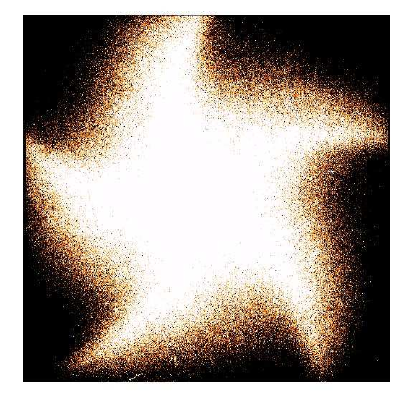
Figure 1: An example of non-uniform CCD illumination caused by a too short t_exp, for an iris-type shutter, obtained with LaRuca@1.5m in San Pedro Mártir, Mexico. The figure shows the ratio between a flat field obtained with a relatively long exposure time (20 sec) and a very short one (0.1 sec): ADU (Analogue-to-Digital Unit) variations of about $\pm$5% are observed from the center to the corners of the image.

To obtain accurate and precise photometry in our survey, we need to characterize two shutter quantities: the shutter delay and the minimum exposure time.

The shutter delay time, also called shutter dead time or shutter offset, is the difference between the requested and the effective t_exp (exposure time). If the shutter closes slower than it opens, the exposure time will be longer than requested, and the shutter delay might be positive, otherwise it is negative. Knowledge of the shutter delay time is necessary for high-precision photometry, where the effective t_exp is needed.

Table 1: Flat field sequences used for the shutter delay, minimum acceptable exposure time, and linearity measurements. The columns contain (see text for more information): (1) the used instrument@telescope combination; (2) the sequence of exposure times used; (3) the exposure time of the monitoring exposures, when available; (4) the used filter or grism; (5) the used slit width in arcseconds, when applicable; (6) the observation date; (7) the experiment for which the measurements were used, with ‘a’ indicating the shutter delay measurement, ‘b’ the minimum acceptable exposure time measurement, and ‘c’ the linearity measurement. Of type $a$ and $c$ observations, the ones taken on 2009 January 29 lack monitoring triplets, because the data were downloaded from the TNG archive.

Instrument	texp	t${}_{\rm{exp}}^{\rm{m}}$	Filter/grism	Slit	Date	Notes
	(sec)	(sec)		(”)	(yyyy Month dd)
BFOSC@Cassini	0.5, 1, 2, 3, 4, 7, 10, 20, 30, 40, 50, 55, 60, 65	5	B	–	2009 May 27	a,b
	6, 26	10	gr7	2	2010 Aug. 30	c
EFOSC2@NTT	10, 60, 120	40	gr3	2	2008 Nov. 26	c
	3, 15, 30	10	gr3	2	2008 Nov. 27	c
	0.1, 0.2, 0.5, 1, 2, 3, 6, 15, 20	10	B	–	2008 Nov. 28	a,b
DOLORES@TNG	5, 20, 55	25	VHR-V	2	2008 Jan. 17	c
	1, 2, 4, 5, 6, 7, 8, 9	–	B	–	2008 Jan. 29	a,b
CAFOS@2.2m	1, 5, 10, 20, 25, 30	15	B200	2	2007 Apr. 01	c
	0.1, 0.5, 1, 2, 3, 4, 5, 6, 20, 30, 40	–	R	–	2008 Apr. 17	b
	0.1, 0.2, 0.5, 1, 2, 3, 4, 5, 6, 15, 20, 30	–	R	–	2008 Sep. 09	b
	0.1, 0.2, 0.4, 0.6, 0.8, 1, 4, 6, 8, 8.7	2	V	–	2010 Sep. 23	a,b,c
LaRuca@1.5m	0.1, 0.2, 0.4, 0.6, 0.8, 1, 2, 3, 4, 10, 20	–	White	–	2008 Aug. 20	b
	1, 2, 4, 8, 15, 18, 20, 25, 30, 35, 36, 37	10	B	–	2008 Aug. 23	a,c
	2, 4, 7, 14, 28, 40, 56, 62, 68, 74, 80, 87, 89	20	R	–	2010 Jul. 17	a,c
	0.2, 0.4, 0.6, 0.8, 1, 2, 3, 4, 5, 6, 10, 15, 20, 30	–	R	–	2010 Jul. 17	b

The minimum acceptable t_exp is set by the finite time the shutter takes to travel from fully closed to fully open (and vice versa). It is not strictly related to the shutter delay. A shutter can have a very small shutter delay (for example because it opens and closes with very similar delays), but it might take some time to completely open. A different shutter can have a significant shutter delay (for example because it starts closing with a significant delay), but it might have a negligible minimum acceptable time because once it starts opening (or closing) it completes the operation in a very short time. Regardless of the shutter delay, a shutter that takes a long time to fully open (or close) might introduce significant illumination non-uniformities across the CCD. To avoid illumination non-uniformities, t_exp must be longer than a safe minimum (see Figure 1 for an example).

2.1 Observations and data reductions

To measure shutter effects, series of imaging flat fields with different exposure times were obtained at each telescope (see Table LABEL:tab:series). Each series consisted of triplets of flats with increasing exposure time, from very short to very long (thus useful for measuring CCD linearity as well, see Section 3). After each triplet, a monitoring triplet with constant exposure time was also taken, to monitor the lamp intensity constancy, following the so-called bracketed repeat exposure method (see Section 3 for more details).

All flat field images were processed with IRAF by correcting them for overscan (where applicable) and subtracting a master bias. For all analyzed instruments the dark currents turned out to be negligible (see Section 4) and no correction for dark was applied. The median of images belonging to the same triplet was computed to remove cosmic ray hits and to reduce the noise.

To correct for lamp drifts, each median image resulting from a monitoring triplet was divided by a reference monitoring triplet (generally the first one of the same sequence), to derive a correction factor. The correction factor was used to correct each triplet — both monitoring and data triplets — and to report them to an ideal ADU level, free of lamp drift variations. The results of this correction are illustrated in Figure 2. The same type of data sequences, extending to longer t_exp, can be used for the CCD linearity characterization described in Section 3, where the lamp drift correction is performed in the same way.

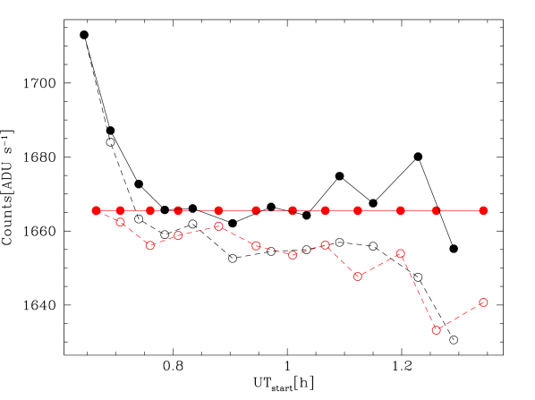
Figure 2: Example of lamp drift correction, based on data obtained with LaRuca@1.5m in August 2008 (see Table LABEL:tab:series). Median ADU per second of each triplet are plotted as a function of time at triplet start. Red symbols represent monitoring triplets, while black symbols represent the actual series triplets. Empty symbols refer to uncorrected triplets, filled symbols to triplets corrected for lamp drift (see Section 2.1). After correction, monitoring triplets are aligned, while data triplets present some residual scatter (less than 1%), presumably caused by residual lamp instability after correction. A non-linear behaviour at low exposure times (left side of the plot) is clearly visible.

2.2 Shutter delay

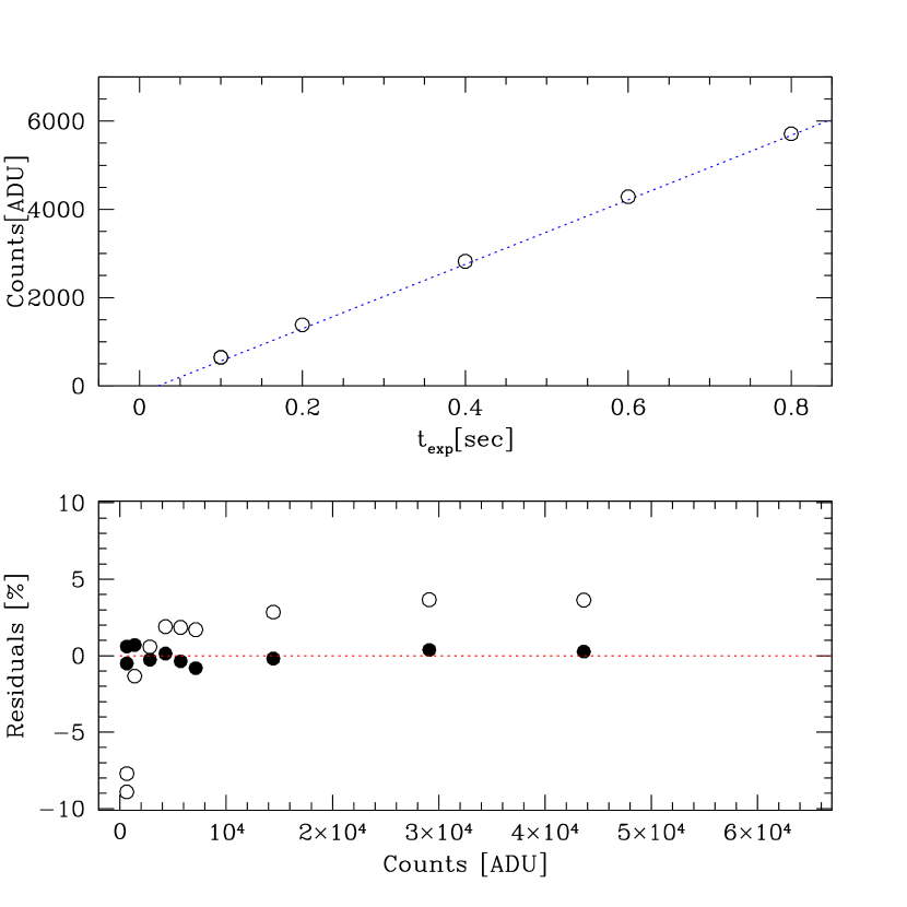
Figure 3: Example of shutter delay determination, for Calar Alto observations obtained on 2010 September 23. Top panel: a zoom into the low t_exp region of the classical ADU versus t_exp plot; the dotted line represents a linear fit of all data and it does not intersect the X axis at zero, but at –0.023 sec. Bottom panel: residuals of the count rate (ADU s^-1) from their average value, as a function of ADU; empty dots are the measured values, while filled dots are corrected for a shutter delay of –0.011 sec. The average of the two determinations, –0.017 sec, is reported in Table LABEL:tab:shutter.

We used two different methods to measure the shutter delay. In the first method, a linear extrapolation of the ADU (Analogue-to-Digital Units) versus t_exp relation crosses the time axis at a value that is generally different from zero, and that corresponds to the shutter delay (Figure 3, top panel). In the second method, the count rate (ADU per second) are plotted versus ADU and should ideally remain constant; in practice, a deviation occurs at low t_exp. By iteratively adjusting the exposure time to $t+\delta t$, the shutter delay corresponds to the $\delta$t that minimizes the residuals from a flat count rate, at the low t_exp end (see also Figure 3, bottom panel). We applied both methods to the data in Table LABEL:tab:series. We obtained consistent values and thus we averaged the results from the two methods to obtain a final shutter delay. Results are reported in Table LABEL:tab:shutter.

2.3 Minimum acceptable exposure time

The effect of illumination variations was estimated by dividing each of the flat fields in a series (Table LABEL:tab:series) by the longest non-saturated flat field in the same series. The resulting ratio images (an example is shown in Figure 1) should have oscillations or variations which are caused by noise only, and no systematic large scale patterns with amplitudes higher than roughly 1%, as required by the Gaia mission calibration goals. The minimum acceptable exposure times, t${}_{\rm{exp}}^{\rm{min}}$, obtained with this criterion are listed in Table LABEL:tab:shutter. While the shutter delay is generally much lower than one second, t${}_{\rm{exp}}^{\rm{min}}$ can be higher than that. We stress the fact that if flat fields acquired with too short t_exp are used to correct all frames of one night, they will affect also scientific images taken with relatively long t_exp, and should thus be avoided.

Table 2: Resulting shutter delays and minimum exposure times for the relevant flat field series in Table LABEL:tab:series. The columns contain (see text for more information): (1) the used instrument@telescope combination; (2), the shutter delay; and (3) the minimum acceptable exposure time.

Instrument	$\delta$t	t${}_{\rm{exp}}^{\rm{min}}$
	(sec)	(sec)
BFOSC@Cassinia	–0.300$\pm$0.050	$\simeq$5
BFOSC@Cassinib	negligible	$\simeq$5
EFOSC2@NTT	+0.008$\pm$0.001	$<$0.1 (if any)
DOLORES@TNG	–0.011$\pm$0.002	$<$1 (if any)
CAFOS@2.2mc	(no data)	3
CAFOS@2.2md	–0.017$\pm$0.070	$<$0.5
LaRuca@1.5m	+0.028$\pm$0.004	5
aValid before 2010 February (see text).
bValid after 2010 February (see text).
cValid before Summer 2008 (see text).
dValid after Summer 2008 (see text).

3 CCD linearity

Linearity is a measure of how consistently the CCD responds to different light intensity over its dynamic range. CCDs can exhibit non-linearities, typically at either or both low and high signal levels (Djorgovski & Dickinson 1989; Walker 1993). High quality CCDs show significant response deviations ($\geq 1$%) from linearity only close to saturation, i.e., at high signal levels when the potential well depth is almost full. Of course the CCD response strongly deviates at saturation, when the potential well depth is full and additional incoming photons do not increase the photoelectrons in a given pixel. When observations are restricted to the linear portion of the dynamic range, the CCD performs as a detector suitable for accurate spectrophotometric measurements.

A few different methods have been presented in the literature to measure and correct for CCD linearity losses, as the bracketed method described by Gilliland et al. (1993), the bracketed repeat-exposure method, and the ratio method described by Baldry et al. (1999). Another method related to the ratio method is described by Leach et al. (1980) and Leach (1987): the variance method. In our Gaia SPSS observing campaigns, we tested the CCD linearity with two methods, described below.

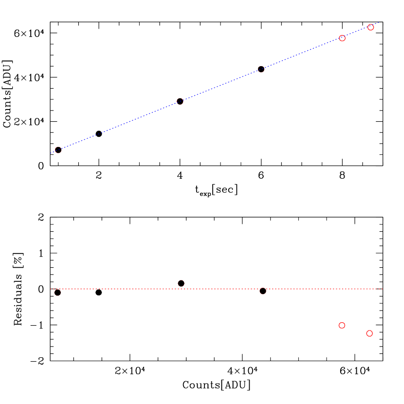
Figure 4: Example of linearity test for Calar Alto observations obtained on 2010 September 23, with the SITE#1d_15 CCD. Top panel: a zoom into the high ADUs region of the classical ADU vs. t_exp plot; the dotted line represents a linear fit of all data. Bottom panel: residuals of the count rate (ADU ^-1) from their average value, as a function of counts; the dotted line represents a constant count rate. In both panels, points deviating by more than 1% are represented by empty circles and coloured in red.

The classical method is based on a series of imaging flat fields with increasing t_exp. Usually, at very high count levels the 1:1 relationship between ADU and t_exp breaks, and an increment of t_exp does not correspond anymore to a fixed increase in ADU (an example can be found in Figure 4). We used the relevant data listed in Table LABEL:tab:series, reduced and corrected for lamp drift as described in Section 2.1. We considered that a deviation of $\geq$1% from linearity was not acceptable given our requirements, and thus we report in Table LABEL:tab:lin the ADU level at which such deviations occur.

Table 3: Resulting maximum acceptable ADU levels obtained from the flat series in Table LABEL:tab:series. The columns contain (see text for more information): (1) the used instrument@telescope combination; (2) the CCD used; (3) the validity period of each CCD; (4) the maximum acceptable ADU level obtained with the classical method; (5) the maximum acceptable ADU level obtained with the Stello et al. (2006) method, when applicable; and (6) the final adopted value for each CCD: when there were no sufficient data, the safe value was assumed conservatively on the basis of that obtained for similar CCDs; in those cases, the values are indicated in parentheses.

Instrument	CCD	Validity period	ADU${}_{\rm{max}}^{\rm{(Classic)}}$	ADU${}_{\rm{max}}^{\rm{(Stello)}}$	ADU${}_{\rm{max}}^{\rm{(Adopted)}}$
BFOSC@Cassini	EEV 1300$\times$1340B (old)	Before 2008 Jul. 17	…	…	(50 000)
	EEV 1330$\times$1340B (new)	After 2008 Jul. 17	…	60 000	60 000
EFOSC2@NTT (1$\times$1 bin)	CCD#40 LORAL/LESSER	All runs (from 2007)	…	49 000	49 000
EFOSC2@NTT (2$\times$2 bin)		All runs (from 2007)	…	47 000	47 000
DOLORES@TNG	E2V 4240 (Marconi)	All runs (from 2007)	60 000	60 000	60 000
CAFOS@2.2m	SITE#1d_15	All runs (from 2007)	55 000	53 000	53 000
LaRuca@1.5m	SITE#1	Until 2009 Jul.	60 000	…	60 000
	ESOPO	2009 Oct. 20–22	…	…	(60 000)
	E2V 4240 (Marconi) #1	2009 Oct. – 2010 Dec.	60 000	…	60 000
	E2V 4240 (Marconi) #2	2011 Mar. 9–17	…	…	(57 000)
	SITE#4	2011 May 2–11	…	…	(60 000)

Table 4: List of grisms used for the SPSS campaigns with the four spectrographs. The columns contain: (i) the instrument@telescope combination; (ii) the grism name; (iii) the minimum wavelength; (iv) the maximum wavelength; (v) the approximate wavelength at which second order contamination starts (if any, see text); (vi) the approximate wavelength at which fringing starts (if any, see text); and (vii) the approximate relative amplitude of the fringing pattern, as measured on our spectra before correcting for fringing. All figures were derived from our SPSS spectra.

Instrument	Grism	$\lambda_{\rm{min}}$	$\lambda_{\rm{max}}$	$\lambda_{\rm{2ndorder}}^{(start)}$	$\lambda_{\rm{fringing}}^{(start)}$	max fringing
		(Å)	(Å)	(Å)	(Å)	($\pm$%)
BFOSC@Cassini	#3	3300	6420	—	—	—
	#5	4800	9800	—	$\simeq$7000	10–15
CAFOS@2.2m	B200	3200	9000	—	—	—
	R200	6300	11000	$>$12000	$\simeq$8500	$\la$5
EFOSC2@NTT	#5	5200	9350	—	$\simeq$7300	$\la$10
	#11	3380	7520	—	—	—
	#16	6015	10320	$\simeq$6000	$\simeq$7300	$\la$10
DOLORES@TNG	LR-B	3000	8430	$\simeq$6000	—	—
	LR-R	4470	10073	$\simeq$9500	$\simeq$8000	5–15

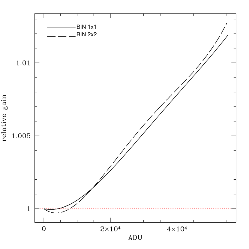
Figure 5: Final gain curves obtained with the Stello et al. (2006) method for NTT, using data obtained on the 26 and 2008 November 27, with 1$\times$1 and 2$\times$2 binning, respectively, with the ESO grism #3. The dashed line is for the 2$\times$2 binning while the solid line is for the 1$\times$1 binning. Very small deviations from linearity start to appear already around 5000 ADU, while deviations above 1% kick in at $\simeq$47 500 ADU for the 2$\times$2 binning and at 49 000 ADU for the 1$\times$1 binning.

The second method we tested is described by Stello et al. (2006), and is a variation on the literature methods described above. It requires the acquisition of at least two spectroscopic flat fields, one reaching the saturation level and the other covering a fainter intensity range. The choice of slit width and grism (or grating) is not crucial, but it is important to obtain flat fields with a wide — and preferably monotonic increasing — intensity range along one direction (either a CCD column or line). The frames were collapsed along the dispersion direction, and corrected for lamp drifts as explained in Section 2.1, but taking into account that lamp drifts in spectra can show also colour variations. Afterwards, we applied the method as described in the original paper by Stello et al. (2006), by computing the intensity ratio of exposure pairs, normalized by their respective t_exp, which is called gain-ratio curve. This ratio is the starting point of an iterative procedure of inversion to determine the gain at different intensity levels.

In conclusion, given our simple purpose of estimating a safe ADU limit for our observations, the classical method and the high-precision method (Stello et al. 2006) give substantially the same results. While the required spectroscopic observations are much faster to obtain, the Stello et al. (2006) method is highly sensitive to different choices for the fit of the gain-ratio curves (function, order, and rejection method), and to their extrapolation at zero counts. Therefore, the method is not as straightforward to apply as the classical method. To estimate the ADU level at which our data deviate more than 1% from linearity, we conservatively chose the lowest of the two estimates, in the few cases where the two methods provided different results. Results for the employed instruments can be found in Table LABEL:tab:lin.

4 Calibration frames

The quality and stability of the calibration frames was tested on all the acquired calibration data, producing recommendations for the calibration plans that were progressively refined as more and more data were available for the analysis. We found a surprising variety of behaviours among different instruments and observing sites. Considering that we acquired of the order of 100 000 frames in our campaigns (see Pancino et al. 2012, for the SPSS campaigns description), it was important to implement automated procedures to identify those calibration frames that needed a closer inspection, before validating the corresponding reduced data. Whenever possible, we acquired daily or nightly calibration frames, but in case of problems, we used the derived calibration plan presented in Table LABEL:tab:plan to decide how to analyze the data (i.e., which of the archival or available frames were acceptable) and how to judge the quality of the applied reductions. In the following sections we briefly describe the monitoring strategy and the main conclusions on each instrument and telescope.

4.1 CCD cosmetics

We employed BPMs (Bad Pixel Masks), i.e., images of the same dimension of the CCD frames, where good pixels are identified by zero values and bad pixels by non-zero values. BPMs were created once or twice a year, using the ratio of two flat fields with different count levels — where pixels responding non-linearly stand clearly out — by means of the IRAF ccdmask task. They were applied with the IRAF task fixpix, which replaces bad pixels with estimates of their correct value. The estimates are built using a linear interpolation across the nearest non-bad pixels, either across lines or columns, or both, depending on the local characteristics of the BPM (see task description for more details), i.e., differently for bad lines, bad columns, or clusters of bad pixels.

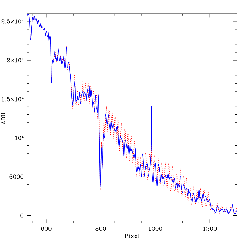
Figure 6: Example of fringing correction (see text) on a spectrum of BD+284211, observed in Loiano on 2013 October 28, with gr5 and a 2.5” slit. The blue solid line is the spectrum after fringing correction, based on a day-time flat, while the red dotted spectrum is before the correction. Beatings are observed, caused by small differences in the fringing pattern of the spectrum and the flat used for the correction. For example, aroud pixel 900 the residuals are below 5%, while around pixel 1000 they remain higher, around 15%.

4.2 Fringing

Fringing, caused by multiple reflections and interferences of red or infrared light in thin CCD substrates (Lesser 1990; Howell 2012), was not relevant for the imaging filters used in our observations (mostly B, V, and R), but was present and relevant in all our spectra, because we needed to cover the whole Gaia wavelength range, from 330 to 1050 nm. All the instruments used for spectroscopy do suffer from fringing (see Table LABEL:tab:grisms), well visible in our spectra (see Figure 6). For NTT we took flat fields very close to our red grism observations, while for all other telescopes we only relied upon day-time lamp flats. However, while flat fielding does reduce the intensity of fringes, the best fringing reduction strategy for spectroscopy, i.e., observing triplets of spectra with the star in different positions along the slit, could not be applied at the chosen telescopes because it would have been too time consuming, observationally.

The solution we adopted was to apply specific spectra processing steps to reduce the impact of fringing, adapting the procedure used in the mkfringeflatcor STIS (Space Telescope Imaging Spectrograph) task for IRAF (Malumuth et al. 2003). Briefly, the most appropriate flat field available for each scientific spectrum was extracted from a region covering exactly the same pixels covered by the scientific spectrum, collapsed to a 1D spectrum along the dispersion direction, and normalized to one. The region that does not contain a significant fringing pattern was then flattened exactly to 1, to avoid adding extra noise to the scientific spectra. Finally, this specially prepared 1D spectroscopic flat was aligned to the scientific spectra and scaled until the residuals of the fringing pattern were minimized, using the IRAF telluric task, and applied to scientific spectra to correct them for fringing.

We found that even using spectroscopic flat fields obtained in the day-time (thus with different incident light patterns), the procedure greatly helps in reducing the amplitude of fringes, up to a factor of 2–3 in relative intensity (see Figure 6). Sometimes, the closeness in position of the day-time flats fringe patterns to the SPSS fringe pattern produced beatings in the residuals of the fringing correction, with regions were the pattern was almost completely erased and regions where a residual fringing pattern remained. This has to be taken into account for applications of the method to scientific cases that could be sensitive to this kind of residual effects.

Additionally, in our spectroscopic campaign we often have observations of the same SPSS from different telescope and observing nights, and thus spectroscopic fringing residuals can be further reduced by building a median of the different spectra. The very red end of spectra ($\lambda\ga$9500 Å), where fringing is strong and S/N is low, will also be replaced with model or semi-empirical template spectra, as done for example by Bohlin (2007).

4.3 Dark frames

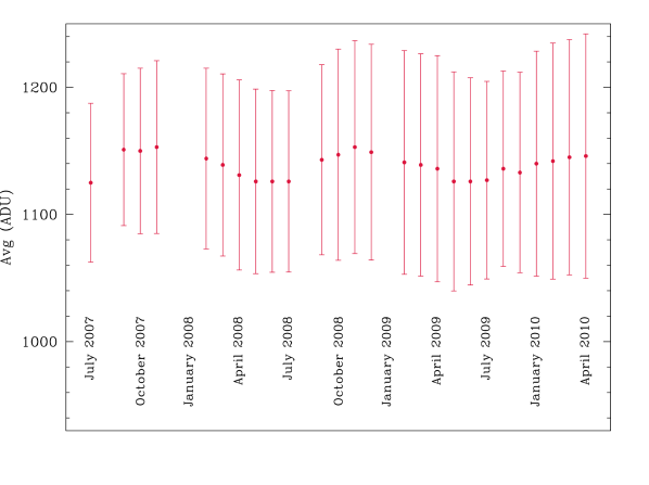
Figure 7: Example of long-term behaviour of the average counts (with their sigma) of REM monthly master dark frames with t_exp=60 s, covering roughly 3 years. A seasonal trend is clearly visible.

Dark correction is the subtraction of the electron counts which accumulate in each pixel due to thermal noise. The reduction of dark currents is the main reason why all astronomical CCDs are cooled to liquid nitrogen temperatures. We took dark exposures as long as the longest scientific exposure, at least once per year. As expected, all used instruments showed at most a few ADU per pixel per hour, except for the REM (Rapid Eye Movement) robotic telescope in La Silla, which is cooled by a Peltier system. The REM staff creates monthly master dark frames, containing the bias structure as well (see below), thus we applied the closest master dark frame in time, taken with the correct t_exp. A seasonal effect on the dark frames average level can be clearly seen in Figure 7, while the 2D shape of the frames was extremely stable and the ADU increased linearly with t_exp.

Table 5: Calibration plan recommendations following our calibration frames monitoring (see text). For each type of calibration frame, the minimum acceptable stability timescale is reported.

Instrument	Dark	Photometric	Spectroscopic	Photometric	Photometric	Spectroscopic	Spectroscopic
		Bias	Bias	Dome Flat	Sky Flat	Lamp flat	Sky flat
BFOSC@Cassini	—	4 days	4 days	300 days	variesc	1 day	1 week
EFOSC2@NTT	—	5 days	1 day	250 days	250 days	1 day	1 week
DOLORES@TNG	—	1 day	1 day	—	250 days	5 days	1 week
CAFOS@2.2m	—	1 week	1 week	variesb	1 day	1 day	1 week
LaRuca@1.5m	—	variesa	—	—	5 days	—	—
ROSS@REMd	1 month	—	—	—	—	—	—
aVaries from 1 to 7 days, depending on the CCD used.
bWas 1 day until Summer 2008, and 1 week afterwards.
cWas 4 days until 2010 February, and 100 days afterwards.
dREM flat fields were not applied, to avoid reinforcing the strong light-concentration effect from which ROSS suffers.

4.4 Overscan and bias frames

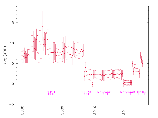
Figure 8: Example of long-term behaviour of the average counts (with their sigma) of San Pedro Mártir daily master bias frames, covering more than three years. The CCD changes are marked and correspond to clear jumps in ADU and also in variations of the ADU stability with time.

The bias current is an offset, preset electronically, to ensure that the Analogue-to-Digital Converter (ADC) always receives a positive value and operates in a linear regime, as much as possible. The offset for each exposure given by the bias level has to be subtracted before further reduction, and may be modelled as $A+B(x_{i},y_{i})$, where $B$ is the pixel-to-pixel variation or 2D structure, which is time-invariant unless particular problems occur, while $A$ is the overall bias level, that can change slightly during the night or even seasonally, owing to temperature changes.

Generally $A$ can be measured using a strip of pixels, called overscan, acquired by continuing to readout the CCD beyond its real physical extent: the result is an oversized array with a strip of signal-free pixels. In our survey, the overscan was available only for DOLORES@TNG and LaRuca@1.5m in San Pedro Mártir, thus in all other cases we used the 2D bias frames to implicitly correct for $A$ as well. This produces some additional uncertainty if $A$ varies during the night, because the bias calibration frames were generally acquired in the afternoon (and also in the morning for the less stable instruments, like LaRuca). The different stability of the four CCDs used with LaRuca is illustrated in Figure 8, where the bias level — after overscan subtraction — of all the master bias frames is plotted.

4.5 Flat fields

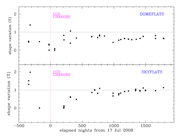
Figure 9: Example of long-term behaviour of the normalized shape variation ($\Delta S/S$, see text) of BFOSC nightly dome (top panel) and sky (bottom panel) flat fields in B filter. The shape variations are rarely above 1%, globally, showing an impressive stability over a period covering more than 2000 nights. The CCD change in Summer 2008 is marked by a vertical dotted line.

After bias subtraction and — if needed — dark correction, data values are directly related to the number of photons detected in each CCD pixel. But different pixels can be characterized by a different sensitivity: the flat fielding correction accounts for the non-uniform CCD response to incident light, that can show variations on all scales, from the whole CCD to the single pixel. In imaging, flat field frames are acquired using the twilight sky or a screen uniformly illuminated by a lamp, with each filter; they are used to correct for sensitivity variations on all scales, acting as a sort of sensitivity map. Massey & Hanson (2013) recommend the use of dome or screen flat fields to correct for the small-scale sensitivity variations and of sky flat fields for large-scale variations. In spectroscopy, only the small scale variations are corrected with flat fields obtained through the spectrograph, i.e., with a slit and a grism (or grating). Of course, flat field frames with low signal or saturated were always rejected (see Section 3).

For imaging flat fields, we were interested in monitoring the large scale shape variations with time. We thus took all the masterframes obtained for each instrument, normalized them by their mode, and smoothed them with a boxcar to remove small scale variations. We then computed a stability function K_stab, using the pixel-to-pixel difference of the counts in each masterflat ($F_{\rm{pix}}$) with respect to a reference masterflat ($F^{\rm{ref}}_{\rm{pix}}$):

$$K_{\rm{stab}}=\sum_{pix=1}^{n}(F_{\rm{pix}}-F_{\rm{pix}}^{\rm{ref}})^{2}$$ (1)

We can then define a normalized shape variation as

$$\frac{\Delta S}{S}=\sqrt{\frac{K_{\rm{stab}}}{K_{\rm{stab}}(1\%)}}$$ (2)

where $K_{\rm{stab}}(1\%)$ is computed in the case where the pixel-to-pixel variation is equal to 1% everywhere. Using this indicator, we have a significant variation (i.e., a global variation above 1%) when $\Delta S/S>1$.

Using the K_stab global indicator, we explored all the master flat fields obtained during our SPSS survey with automatic procedures (see Figure 9 for an example), thus identifying the flat fields that needed to be visually inspected for anomalies, before applying them to the scientific images.

4.5.1 Illumination variations

For imaging, dome and sky flat fields are sufficient to correct for the CCD response variations (Massey 1997; Massey & Hanson 2013). Instrumental effects, like internal light reflections or light concentration, need instead ad hoc procedures (Manfroid, Selman, & Jones 2001; Koch et al. 2004). Among the imagers used in the SPSS campaigns, only ROSS@REM showed a significant (up to 5–10%, depending on the amount of incident light) cushion-shaped illumination variation, that was worsened by the application of the flat-field correction, similarly to what happens with light concentration. Because ROSS@REM was only used for relative photometry, we decided not to apply any flat-field correction to REM images and to keep the SPSS as much as possible in the same X and Y position in the CCD during each time series. Nevertheless, relative photometry with ROSS@REM proved to be extremely difficult and only rarely met our requirement of $\sim$millimag accuracy.

For spectroscopy, illumination variations caused by imperfections on the slit borders, vignetting, and other similar effects, are usually corrected with the help of twilight sky spectroscopic flat fields (Massey & Hanson 2013; Schönebeck et al. 2014), applied after normal (i.e., lamp) flat fielding. After some initial testing, we decided to obtain spectroscopic flats fields once per run, as a compromise between the stability of the results and the time needed to obtain the flats (see Table LABEL:tab:plan).

5 Lamp flexures

Low resolution spectrographs are usually mounted at the telescope or at the telescope derotator, and they move during observations. At each different position, the varying projection of the gravitational force leads to mechanical distortions, which can be seen on the wavelength calibration frames, where they produce linear or non-linear shifts of the lamp emission lines (Munari & Lattanzi 1992). A correct flux table must associate the right flux to the right wavelength, thus any error in wavelength has an impact on the flux calibration of a spectrum.

We performed a test to evaluate the DOLORES@TNG lamp flexures on 2008 January 31, when the instrument was equipped with three separate calibration lamps (He, Ne, Ar) that could not be switched on simultaneously, and the procedure to obtain high S/N calibration lamps for each single star during night-time observations was too time consuming. We used the LR-R grism, the 2” slit and the Ar lamp. Triplets of wavelength calibration lamp spectra were acquired at different positions of the derotator, covering a complete derotator circle, from -260 to + 100 degrees in steps of 10 degrees forward, and from +95 up to -255 degrees in steps of 10 degrees backwards. The median of the three acquired lamp frames at each position was used to evaluate line shifts.

The resulting shifts of emission lines, as a function of derotator angle, are characterized by a quasi-sinusoidal trend, as shown in Figure 10 for a selection of the examined lines. The typical size of the global oscillation was almost three pixels, with an error on the lines peak position ranging from 0.01 pixels in the central portion of the CCD to 0.06 pixels at the CCD borders. The shift amounts to almost 8 Å  in the space of wavelengths and thus daytime lamps are clearly not appropriate for the wavelength calibration of spectra in the Gaia spectrophotometric campaigns. For this reason, most astronomers also take wavelength calibration lamps close to the position of each observed spectrum. Not being able to measure emission line shifts for all instruments, we also adopted the same strategy. In particular, if the night lamp observations required too much time — as was initially the case with TNG — we decided to employ day-time lamps with very high S/N, and shift them to match the night lamps taken with lower S/N in order to save time. In all other cases we used night-time lamps.

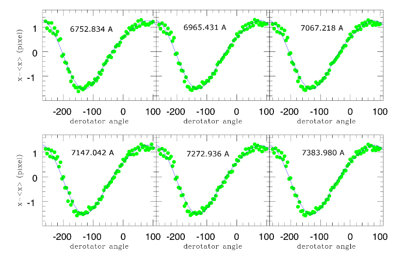
Figure 10: Example of lamp flexure effect on emission lines position of a TNG Argon wavelength calibration lamp exposure with the LR-R grism (see text). Each panel represents the line peak shift in pixels (ordinate) of six individual argon lines as a function of DOLORES derotator angle position (abscissa). Each green dot corresponds to a peak measurement in a different lamp exposure. The typical shift of almost $\pm$1.5 pixels corresponds to almost 8 Å. The thin black line is a polynomial fit to the data, to guide the eye.

6 Polarization

The reflectivity of curved and plane mirrors may be different for different directions of linear polarization, in a wavelength dependent way (see Breckinridge & Oppenheimer 2004, and references therein). An incoming beam of non-polarized light will be polarized according to this difference of efficiency. This might affect the sensitivity of the whole observing system, especially if the light beam encounters other polarization-sensitive optical elements after reflection. The degree of induced polarization depends on the angle of incidence: the maximum degree of (linear) polarization occurs for an incidence angle which depends on the material, called polarization angle. Refractive dispersing elements (grisms, in our case) may also — in principle — produce some degree of polarization, or may have different transmission efficiencies for different intrinsic polarization of the incoming light, thus introducing selective light losses. A combination of optical elements with different orientation could thus produce a significant variation in the efficiency, dependent on wavelength and/or pointing.

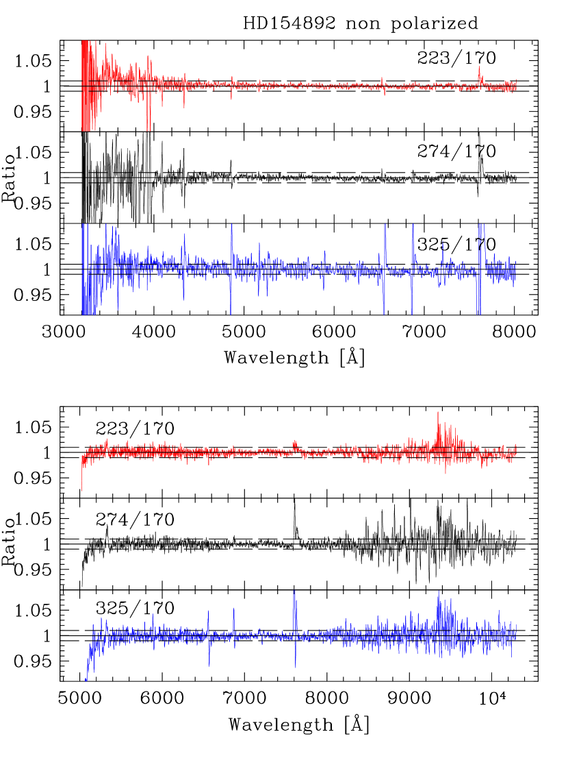
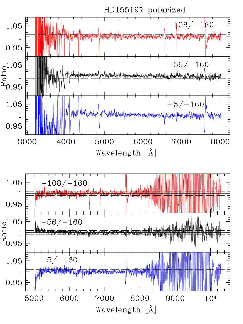
Figure 11: Results of our test on the effect of polarization on spectrophotometry. The left panels report observations of the “non-polarized” star HD 154892. while the right panels of the “polarized” star HD 155197 (see text for more details). The three top panels for each star refer to the LR-B grism, while the bottom panels to the LR-R grism. Each sub-panel shows the ratio of spectra taken at different derotator angles with respect to a reference angle, which is 170 deg for the non-polarized star and –160 deg for the polarized star. All ratios are shown as a function of wavelength. Dashed lines in each sub-panel indicate $\pm$1% ratio variations. Except for the noisy blue edge, and the red parts were fringing is important, it is clear that the effect is negligible for our purposes. The increase in the fringing residuals pattern for the polarized star is caused by the fact that the polarized star was accidentally placed in different positions along the slit for different polarization angles.

We can envisage three cases relevant to our SPSS campaigns:

1. The light beam encounters just one optical element potentially sensitive to polarization, for example the grism, as in the case of CAFOS@2.2m in Calar Alto. If the incoming light is polarized, there may be a difference in the response depending on the actual orientation of the grism in the plane perpendicular to the direction of the light beam. If the incoming light is not polarized, there is no effect.

2. There is more than one element potentially sensitive to polarization, but their relative orientation in the planes perpendicular to the direction of the incoming beam are fixed, as is the case of the flat mirror feeding the grisms of BFOSC@Cassini. The net result is the same as above.

3. There is more than one element potentially sensitive to polarization, and their relative orientation in the planes perpendicular to the direction of the incoming beam changes, depending on the telescope pointing. This is the case of the flat M3 mirror of the twin TNG and NTT telescopes that drives the main light path to the Nasmyth focus where it feeds the grism of the DOLORES and EFOSC2 spectrographs, mounted on the derotator device. In this case some polarization effect can be induced even on non-polarized incoming light, and the grism may respond slightly differently — in terms of efficiency — to differently polarized light, resulting in a light loss depending on the relative orientation of the two elements (see Giro et al. 2003).

6.1 The TNG polarization experiment

While potentially highly polarized sources should be avoided as candidate SPSS (as for instance DP white dwarfs or heavily extincted stars), there is no observational strategy that can completely avoid the problem. We thus tested the above hypothesis on TNG, because it has the same NTT design, and they are the only two telescopes in our campaign where polarization could significantly affect spectro-photometric observations.

We observed two stars from Turnshek et al. (1990): HD 155197, which exhibits a polarization in V band of 4.38$\pm$0.03 % — that we will call polarized star hereafter — and HD 154892, having a B-band polarization of 0.05$\pm$0.03 % — that we will call non-polarized star. They were observed on a clear night (2012 June 1, kindly obtained by the TNG staff), with good seeing (0.8”–1.5”), using a wide slit (10”) and the same grisms used for the SPSS campaign (LR-R and LR-B, see Table LABEL:tab:grisms). Spectra were taken at different derotator angles of –160, –108, –56, and –5 degrees for the polarized star, and 170, 223, 274, and 325 degrees for the non-polarized star. The spectra were bias and flat-field corrected, extracted, and calibrated in wavelength with the help of narrow slit (2”) spectra and day-time calibration lamps, using standard recipes from the IRAF apall and onedspec packages, configured exactly as done for our SPSS reductions (Cocozza et al. 2013). We finally corrected all spectra for atmospheric extinction, using an extinction curve built from our own data, even if the airmass difference among the used spectra was small: 0.10 for the polarized star and 0.05 for the non-polarized star.

As can be seen in Figure 11, the overall shapes of the spectra taken at different derotator angles agree with one another within 1%, except at the blue edge (below 4000 Å), where the S/N is rather low, and above 8000 Å, as expected because of fringing and telluric absorption (which were not corrected for in this particular test). This confirms first of all that the night conditions were photometric. The additional absence of significant slopes or oscillations confirms that both the stellar intrinsic polarization and the polarization supposedly induced by the instrument configuration had no significant impact on our flux measurements (i.e., not more than 1%), even for different stellar polarization levels, wavelength regions, or derotator positions.

7 Second-order contamination

Low resolution spectrographs and large format CCDs allow for observations of a wide wavelength range, as needed for the Gaia SPSS grid. However, with both grisms and gratings the light from different orders can overlap, especially if no cross disperser or blocking filter is employed (Gutierrez-Moreno et al. 1994). Typically, light from the blue wavelengths of the second order can contaminate the red portion of the spectra, in the spectrographs used in our campaign. The characteristics of the contaminating light depend on both the spectral energy distribution of the observed source and the characteristics of the dispersing element. In particular, it is necessary to know the grism (Traub 1990) or grating (Szokoly et al. 2004) equation to apply a correction.

Two of our adopted instrument configurations, for EFOSC2@NTT and DOLORES@TNG, are known to possess significant second order contamination. For CAFOS@2.2m in Calar Alto the only visible second order light started well after 10 000 Å, after the end of the first-order spectrum in the red. For BFOSC@Cassini it was absent, both judging from the BFOSC manuals and web pages, and from the quality of our final spectra of CALSPEC stars. The chosen setups were unavoidable owing to our requirements to cover as much as possible the Gaia wavelength range (300-1100 nm) and to oversample the resolution of the BP and RP (Blue and Red Photometers) by a factor of up to 4–5, whenever possible.

We thus employed an adaptation of the method by Sánchez-Blázquez et al. (2006) to correct our spectra from second-order contamination. The original method requires observations of a blue and a red star, with well known calibrated flux in the literature. They are used to build a response curve for the contaminating second-order spectra, by solving the following system of equations:

$$S_{b}=C_{1}T_{b}+C_{2}T_{2b}$$ (3)

$$S_{r}=C_{1}T_{r}+C_{2}T_{2r}$$ (4)

where the $b$ subscript refers to the blue star and the $r$ one to the red star. $S$ is the observed spectrum, including the second-order contamination, while $T$ is the true spectrum obtained from the literature (thus free from second-order contamination), and $T_{2}$ is the second-order contaminating component. $C_{1}$ is the response curve for the first order light and $C_{2}$ for the second order light: once they are known, any spectrum observed with the same instrument can be corrected for second-order contamination as described by Sánchez-Blázquez et al. (2006). Since $C_{1}$ and $C_{2}$ were not computed each night in our SPSS campaign, we derived the corrected spectrum ($S^{\prime}_{b}$ for the blue star case) using

$$S^{\prime}_{b}=S_{b}-C_{2}S^{\prime}_{2b}$$ (5)

where $S^{\prime}_{2b}$ is the ratio $S_{b}/C_{1}$, i.e., the second order contaminating spectrum, after resampling and shifting, according to the function mapping the first order into the second order wavelength range (see following sections for more details), and still not calibrated in flux.

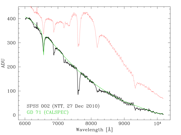
Figure 12: Example of our second order contamination correction for a CALSPEC star (GD 71, one of the pillars) observed with NTT. The red (dotted) spectrum is our observed spectrum contaminated by second-order light coming from blue wavelengths. The black spectrum is the same spectrum after our second order correction procedure; it still contains telluric absorption bands and fringing. The green spectrum is the CALSPEC spectrum for the same star: the spectral shape is recovered to the 1% level.

The method by Sánchez-Blázquez et al. (2006) requires a single spectrum to cover the whole wavelength range, while in our case we always had two setups — with some overlap — observed in two slightly different moments of time. Our adaptation consisted in joining the blue and red spectra of the observed stars, after reporting the blue spectrum to the airmass of the red one with a good extinction curve. A residual jump in the junction point does not have any effect on the quality of the final correction for second order.

While the original method by Sánchez-Blázquez et al. (2006) for deriving $C_{1}$ and $C_{2}$ can be applied directly, even in non-perfectly photometric conditions, our particular adaptation requires some care in those cases where extinction vatiations are large. Application of the method is safe in photometric and grey nights, where extinction variations are lower than $\simeq$3%, roughly speaking.

7.1 NTT second order correction

The spectra of two well known flux standards, Feige 110 (a blue star, Landolt & Uomoto 2007) and LTT 1020 (a red star, Landolt 1992), where acquired with the blue and red EFOSC2 grisms #11 and #16 (see Table LABEL:tab:grisms), used for the whole SPSS campaign. Each star was observed with a 10” slit to gather all the flux, and with a 2” slit to obtain a reliable wavelength calibration.

The spectra were extracted and wavelength calibrated as described in Section 6.1. We created an extinction curve from our own data, that compared well with the CTIO and ESO ones. We then joined the grism #11 and #16, reported to the same airmass, into a single spectrum, cutting them at 6000 Å, i.e., well before the expected start of second order contamination. We used the absorption lines of the blue contaminating spectrum — well visible at red wavelengths — to determine the function that maps the blue contaminating wavelengths in the red wavelength domain:

$$\lambda_{2}=-3815+3.271~{}\lambda_{1}-0.0001167~{}\lambda_{1}^{2}$$ (6)

where $\lambda_{1}$ is the wavelength in Å of the first order, and $\lambda_{2}$ the corresponding wavelength of the second-order contaminating blue light. The residuals around this fit were of 2.9 Å. The flux reference tables used for computing the response curves, i.e., $T_{b}$ and T_r in the equations of the previous section, were obtained for LTT 1020 from CTIO (Hamuy et al. 1992, 1994) and for Feige 110 from the CALSPEC database (Bohlin, Dickinson & Calzetti 2001).

Once the two response curves $C_{1}$ and $C_{2}$ were derived, we computed the percentage of the blue light of a star that is expected to fall at each red wavelength, as

$$P=\frac{C^{\prime}_{2}}{C_{1}}$$ (7)

where $C^{\prime}_{2}$ is $C_{2}$ reported into blue wavelengths using the relation above. The computation of $P$ was repeated in two different epochs (using LTT 1020 and Feige 110 on 2008 November 30, and LTT 9239 and Feige 110 on 28 August 2011) and appeared stable within 1%. The contamination starts around 6 000Å, as shown in Figure 12, and becomes severe around 6 500Å.

7.2 TNG second order correction

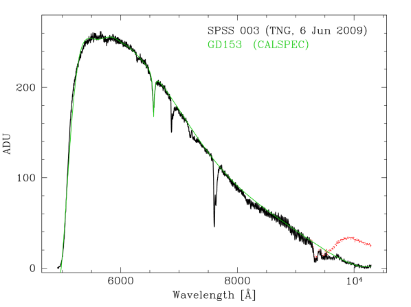
Figure 13: Same as Figure 12, but for one TNG spectrum of GD 153, taken in 2009 June. Apart from the telluric bands and the strong fringing that was not corrected for at this stage, the second order contamination — starting around 9000-9500 Å  — is very well corrected even with our simple assumptions on the grism equation (see text).

The DOLORES red LR-R grism used in our SPSS campaign had a built-in order-blocking filter for wavelengths bluer than $\simeq$5 000 Å, but unfortunately some second-order contamination from blue light was observed after $\simeq$9500 Å To obtain the percentual contamination, $P$, we used two well known standards: HZ 44 (a blue star, Landolt & Uomoto 2007) and G 146-76 (a red star, Høg et al. 2000). A third star, GD 153 (another blue star, Bohlin, Colina & Finley 1995) was observed to independently test the results. We also observed all LR-R spectra together with the Johnson I broadband filter in front of the spectrograph, to recover independently the uncontaminated spectral shape. They were observed with the LR-B and LR-R grisms (see Table LABEL:tab:grisms) both with a 5” slit, the widest available at the time, and with the 2” slit for a better wavelength calibration. We also tested GD 153 and KF06T2 (Reach et al. 2005) on 2009 June 8 with similar results: the maximum difference between the two $P$ curves was always lower than $\simeq$0.3%. All spectra were extracted and wavelength calibrated as in the NTT case, and reported to the same airmass with a tabulated extinction curve. We joined the spectra arbitrarily at 5850 Å, i.e., well before the start of second-order contamination.

To determine a wavelength mapping relation, we obtained helium lamp spectra, with 1 h t_exp, with a B filter to block first order light. Of the three measureable emission lines in LR-R, one was at 9553 Å, where no He line is expected. We thus could not derive a good fit of the function mapping the second order, as done for the NTT case. We used the simple formula $\lambda_{1}=2\lambda_{2}$, that derives from the simplest form of the grating equation

$$m\lambda=\sigma(\sin\beta\pm\sin\alpha)$$ (8)

We then derived the C₁ and C₂ curves and the percentage of contaminating flux using this basic assumption: the emission line appearing at 9553 Å  corresponded well with the 4713 Å  He emission line.

We tested the correction on TNG observations of various CALSPEC and literature standards (one example is reported in Figure 13). We obtained good results, having differences with SPSS literature spectra of 1–2% at most, for several stars. However, the presence of fringing and a deep telluric band in the contaminated region (after 9500 Å) causes high residuals, which can be $\la$10% in the worst cases. For many SPSS we had observations from other telescopes, but for the few SPSS observed only with TNG, a viable solution will be to replace the flux tables after 9500 Å  with model spectra (see also Bohlin 2007).

8 Conclusions

To build a grid of $\sim$100 SPSS with $\leq$1% internal errors and $\leq$1–3% external errors (with respect to the Vega calibration by Bohlin 2007) we have carried out a systematic study of instrumental effects that could have an impact on the flux calibration of SPSS flux tables and integrated magnitudes, finding methods to beat each effect separately down, until their impact on fluxes (or ADUs) was below 1%. We collected from the literature the available methods and strategies to both evaluate and remove those instrumental effects, and carried out specific daytime and nighttime observations to quantify their effects. When necessary, we adapted the methods to our case, or developed our specific tests and data-reduction methods. Whenever feasible — given the difficulties to obtain telescope time for such programs — we compared different approaches to the same problem. In particular:

• we characterized the employed CCDs to evaluate their minimum acceptable exposure time, the shutter delay, and the linearity limit, using different methods, and deriving recommendations for our SPSS observing campaigns (see Tables LABEL:tab:shutter and LABEL:tab:lin);

• we carried out a calibration frames monitoring plan, that provided recommendations on the minimum frequency of each calibration type observations (see Table LABEL:tab:plan) for our observations;

• as part of our calibration frames monitoring, we devised a specific procedure to correct our spectra for fringing, after manipulation of spectroscopic flat fields (following the strategy by Malumuth et al. 2003) and using the IRAF telluric task;

• we have also quantitatively studied the effect of gravity-induced lamp flexures at DOLORES@TNG; we found shifts of about 3 pixels, with 0.01-0.06 errors, corresponding to almost 8 Å  in the wavelength space, confirming that for this type of instruments day-time lamps are not sufficiently accurate. If night-time lamps required too much observing time, we acquired high S/N day-time lamps and shifted them onto the night-time ones to perform the wavelength calibration;

• we studied the effect of instrument-induced polarization with both NTT and TNG, the two instruments that should have the largest polarization in our SPSS campaigns. We observed stars with polarization levels up to 4% at different instrument rotation angles, and concluded that even in the case of SPSS with those intrinsic polarization levels, the flux calibration remained stable within 1%;

• we tested and adapted to our case the method described by Sánchez-Blázquez et al. (2006) to correct our spectra for second order contamination; our method can be applied in photometric and grey nights with residuals generally within 1-2% for NTT and TNG.

In summary, a few of the examined instrumental effects turned out to be negligible, while we devised specific methods to correct for the remaining ones, reducing their impact on the flux calibration of SPSS magnitudes and spectra to $\leq$1%. The methods can be applied to a wide range of observational programs on similar instruments.

The actual reduction and analysis of the SPSS spectra will be presented in a subsequent paper, where we will further reduce the residuals of instrumental effect corrections by combining several independent observations for each SPSS. We will also replace the low S/N blue and red borders (roughly $\leq$3800–4000 Å  and $\geq$9500 Å) with theoretical or semiempirical templates.

References

- Altavilla et al. (2011) Altavilla, G., Pancino, E., Marinoni, S., Cocozza, G., Bellazzini, M., Bragaglia, A., Carrasco, J. M., Federici, L.: 2011, Gaia Technical Report No. GAIA-C5-TN-OABO-GA-004
- Altavilla et al. (2012) Altavilla, G., Botticella, M. T., Cappellaro, E., Turatto M.: 2012, Ap&SS 341, 163
- Altavilla et al. (2014) Altavilla, G., Ragaini, S., Pancino, E., Cocozza, G., Bellazzini, M., Galleti, S., Marinoni, S.: 2014, Gaia Technical Report No. GAIA-C5-TN-OABO-GA-005
- Bailer-Jones et al. (2013) Bailer-Jones, C. A. L., Andrae, R., Arcay, B., et al.: 2013, A&A 559, 74
- Baldry et al. (1999) Baldry, I. K., Viskum, M., Bedding, T. R., Kjeldsen, H., Frandsen, S.: 1999, MNRAS 302, 381
- Breckinridge & Oppenheimer (2004) Breckinridge, J. B., Oppenheimer, B. R.: 2004, ApJ 600, 1091
- Bohlin, Colina & Finley (1995) Bohlin, R. C., Colina, L., Finley, D. S.: 1995, AJ 110, 1316
- Bohlin, Dickinson & Calzetti (2001) Bohlin, R. C., Dickinson, M. E., Calzetti, D.: 2001, AJ 122, 2118
- Bohlin (2007) Bohlin, R. C.: 2007, ASPC 364, 315
- Bohlin, Gordon, & Tremblay (2014) Bohlin, R. C., Gordon, K. D., Tremblay, P.-E.: 2014, PASP 126, 711
- Busonero et al. (2006) Busonero, D., Gai, M., Gardiol, D., Lattanzi, M. G., Loreggia, D.: 2006, A&A 449, 827
- Carrasco et al. (2007) Carrasco, J. M., Jordi, C., Lopez-Marti, B., Figueras, F., Anglada-Escude, G.: 2007, Gaia Technical Report No. GAIA-C5-TN-UB-JMC-002
- Cocozza et al. (2013) Cocozza, G., Altavilla, G., Carrasco, J. M., Pancino, E., Marinoni, S., Galleti, S.: 2013, Gaia Technical Report No. GAIA-C5-TN-OABO-GCC-001
- Djorgovski & Dickinson (1989) Djorgovski, S., Dickinson, M.: 1989, HiA 8, 645
- Gilliland et al. (1993) Gilliland R. L., Brown, T. M., Kjeldsen, H., et al.: 1993, AJ 106, 2441
- Giro et al. (2003) Giro, E., Bonoli, C., Leone, F., Molinari, E., Pernechele, C., Zacchei, A.: 2003, SPIE 4843, 456
- Gullixson (1992) Gullixson, C. A.: 1992, ASPC 23, 130
- Gutierrez-Moreno et al. (1994) Gutierrez-Moreno, A., Heathcote, S., Moreno, H., Hamuy M.: 1994, PASP 106, 1184
- Jordi et al. (2010) Jordi, C., Gebran, M., Carrasco, J. M., et al.: 2010, A&A 523, 48
- Hamuy et al. (1992) Hamuy, M., Walker, A. R., Suntzeff, N. B., Gigoux, P., Heathcote, S. R., Phillips, M. M.: 1992, PASP 104, 533
- Hamuy et al. (1994) Hamuy, M., Suntzeff, N. B., Heathcote, S. R., Walker, A. R., Gigoux, P., Phillips, M. M.: 1994, PASP 106, 566
- Howell (2012) Howell, S. B.: 2012, PASP 124, 263
- Høg et al. (2000) Høg, E., Fabricius, C., Makarov, V. V., et al.: 2000, A&A 357, 367
- Koch et al. (2004) Koch, A., Odenkirchen, M., Grebel, E. K., Caldwell, J. A. R.: 2004, AN 325, 299
- Landolt (1992) Landolt, A. U.: 1992, AJ 104, 340
- Landolt & Uomoto (2007) Landolt, A. U., Uomoto, A. K.: 2007, AJ 133, 768
- Leach et al. (1980) Leach, R. W., Schild, R. E., Gursky, H., Madejski, G. M., Schwartz, D. A., Weekes, T. C.: 1980, PASP 92, 233
- Leach (1987) Leach, R. W.: 1987, OptEn 26, 1061
- Lesser (1990) Lesser, M. P.: 1990, ASPC 8, 65
- Lindegren et al. (2008) Lindegren, L., Babusiaux, C., Bailer-Jones, C., et al.: 2008, IAUS 248, 217
- Malumuth et al. (2003) Malumuth, E. M., Hill, R. S., Gull, T., et al.: 2003, PASP 115, 218
- Manfroid, Selman, & Jones (2001) Manfroid, J., Selman, F., Jones, H.: 2001, Msngr 104, 16
- Marinoni (2011) Marinoni, S.: 2011, PhDT, Bologna University
- Marinoni et al. (2012) Marinoni, S., Pancino, E., Altavilla, G., Cocozza, G., Carrasco, J. M., Monguió, M., Vilardell, F.: 2012, Gaia Technical Report No. GAIA-C5-TN-OABO-SMR-001
- Marinoni et al. (2013) Marinoni, S., Galleti, S., Cocozza, G., Pancino, E., Altavilla, G.: 2013, Gaia Technical Report No. GAIA-C5-TN-OABO-SMR-002
- Massey (1997) Massey, P.: 1997, iraf.noao.edu/iraf/docs/ccduser3.ps.Z
- Massey & Hanson (2013) Massey, P., Hanson, M. M.: 2013, pss2.book, 35
- Mignard (2005) Mignard, F.: 2005, ASPC 338, 15
- Mignard et al. (2008) Mignard, F., Bailer-Jones, C., Bastian, U., et al.: 2008, IAUS 248, 224
- Munari & Lattanzi (1992) Munari, U., Lattanzi, M. G.: 1992, PASP 104, 121
- Newberry (1991) Newberry, M. V.: 1991, PASP 103, 122
- Oke (1990) Oke, J. B.: 1990, AJ 99, 1621
- Pakštiene & Solheim (2003) Pakštiene, E., Solheim, J.-E.: 2003, BaltA 12, 221
- Pancino et al. (2008) Pancino, E., Altavilla, G., Bellazzini, M., Marinoni, S., Bragaglia, A., Federici, L., Cacciari, C.: 2008, Gaia Technical Report No. GAIA-C5-TN-OABO-EP-001
- Pancino et al. (2009) Pancino, E., Altavilla, G., Carrasco, J. M., et al.: 2009, Gaia Technical Report No. GAIA-C5-TN-OABO-EP-003
- Pancino et al. (2011) Pancino, E., Altavilla, G., Carrasco, J. M., Marinoni, S., Cocozza, G., Bellazzini, M., Federici, L.: 2011, Gaia Technical Report No. GAIA-C5-TN-OABO-EP-006
- Pancino et al. (2012) Pancino E., Altavilla, G., Marinoni, S., et al.: 2012, MNRAS 426, 1767
- Perryman et al. (2001) Perryman, M. A. C., de Boer, K. S., Gilmore, G., et al.: 2001, A&A 369, 339
- Prusti (2011) Prusti T.: 2011, EAS 45, 9
- Prusti (2012) Prusti, T.: 2012, AN 333, 453
- Reach et al. (2005) Reach W. T., Megeath, S. T., Cohen, M., et al.: 2005, PASP 117, 978
- Sánchez-Blázquez et al. (2006) Sánchez-Blázquez P., Peletier, R. F., Jiménez-Vicente, J., et al.: 2006, MNRAS 371,703
- Wenger et al. (2000) Wenger M., Ochsenbein, F., Egret, D., et al.: 2000, A&AS 143, 9
- Schönebeck et al. (2014) Schönebeck, F., Puzia, T. H., Pasquali, A., Grebel, E. K., Kissler-Patig, M., Kuntschner, H., Lyubenova, M., Perina, S.: 2014, A&A 572, 13
- Soubiran et al. (2013) Soubiran, C., Jasniewicz, G., Chemin, L., Crifo, F., Udry, S., Hestroffer, D., Katz, D.: 2013, A&A 552, 64
- Stello et al. (2006) Stello D., Arentoft, T., Bedding, T. R, et al.: 2006, MNRAS 373, 1141
- Sullivan et al. (2011) Sullivan, M., Guy, J., Conley, A., et al.: 2011, ApJ 737, 102
- Szokoly et al. (2004) Szokoly, G. P., Bergeron, J., Hasinger, G., et al.: 2004, ApJS 155, 271
- Traub (1990) Traub, W. A.: 1990, JOSAA 7, 1779
- Turnshek et al. (1990) Turnshek, D. A., Bohlin, R. C., Williamson, R. L. II, Lupie, O. L., Koornneef, J., Morgan, D. H.: 1990, AJ 99, 1243
- Tyson (1990) Tyson J. A.: 1990, ASPC 8, 1
- van Leeuwen & Richards (2012) van Leeuwen, F., Richards, P.: 2012, Gaia Technical Report No. GAIA-C5-TN-IOA-FVL-001
- Walker (1993) Walker, A. R.: 1993, spct.conf, 278