Detecting breaks in the dependence of multivariate extreme-value distributions
Abstract
In environmental sciences, it is often of interest to assess whether the dependence between extreme measurements has changed during the observation period. The aim of this work is to propose a statistical test that is particularly sensitive to such changes. The resulting procedure is also extended to allow the detection of changes in the extreme-value dependence under the presence of known breaks in the marginal distributions. Simulations are carried out to study the finite-sample behavior of both versions of the proposed test. Illustrations on hydrological data sets conclude the work.
Keywords and Phrases: copula; hydrological applications; multivariate block maxima; Pickands dependence function; resampling; sequential empirical processes.
1 Introduction
The study of extremes is of importance in many environmental applications. Prominent examples are the analysis of floods (Hosking and Wallis, 2005), heavy rainfalls (Cooley et al., 2007) and extreme temperatures (Katz and Brown, 1992). Many of these problems are intrinsically multivariate; for instance, the severity of a flood depends not only on its peak flow, which is considered in many univariate flood studies, but also on its volume and its duration (Yue et al., 1999). Catastrophic flood events typically occur when more than one of these variables is taking a high value and therefore, the analysis of the joint behavior is of key importance. In a river system, where flood data are collected from a number of stations, inference at a specific location can be greatly improved by incorporating observations from neighboring stations (Hosking and Wallis, 2005). Similarly, extreme temperatures are commonly studied at several stations simultaneously.
In most of these environmental applications, it is common practice to assess the extreme observations by (modifications of) the annual block maxima method, popularized in the classical monograph by Gumbel (1958). Univariate observations collected on, say, a daily basis are aggregated by taking maxima over a longer time period, usually a year for stationarity considerations, resulting in a sample of maxima capturing most of the extreme outcomes. Thanks to the extremal types theorem, univariate block maxima are approximately distributed according to the (parametric) generalized extreme distribution, while the dependence within a vector of block maxima can be described approximately by a (nonparametric) extreme-value copula (de Haan and Ferreira, 2006). The resulting joint distributions are called multivariate extreme-value distributions and serve as a widely accepted model for multivariate block maxima.
In statistical applications, it is common practice to assume that the time series of block maxima is stationary, temporarily independent and that its stationary distribution is exactly of the extreme-value type. Except for stationarity, the above assumptions are theoretically justified by the results of Bücher and Segers (2014) if the focus is solely on the dependence structure. In the current paper, we address the issue of stationarity by developing tests for change-point detection within the multivariate contemporary distribution.
More precisely, assuming that we observe a sample of independent multivariate observations , where each follows a multivariate extreme-value distribution whose c.d.f. is denoted , we develop a test for the hypothesis
| (1.1) |
against alternatives involving the non-constancy of the c.d.f.s. Since the univariate version of this problem has been treated, for instance, in Jaruškova and Rencová (2008) using results from Chapter 1 of Csörgő and Horváth (1997), we will be particularly interested in the multivariate setting throughout this paper.
Outside of the extreme-value framework, there is a huge amount of literature on detecting deviations from , see the classical monograph of Csörgő and Horváth (1997) or Aue and Horváth (2013) for a recent review. It is useful to note that, by Sklar’s theorem (Sklar, 1959), we can rewrite as , where
| (1.2) | ||||
| (1.3) |
Roughly speaking, tests for can be divided into two groups: tests that are powerful against deviations from but which are rather insensitive to deviations from , and vice versa, see Bücher et al. (2014) for a discussion. In the present setting of observing data from a multivariate extreme-value distribution, the tests considered for instance in Jaruškova and Rencová (2008) can be used to detect deviations from , whence it will be our main concern to design a test that is particularly sensitive to deviations from when is known to be an extreme-value copula. Note that none of the existing tests for changes in the copula (see, e.g., Bücher et al., 2014; Kojadinovic et al., 2015, among others) incorporates the latter information, whence an improvement in the power properties seems possible. In fact, our simulation study partially reported in Section 5 suggests that our proposed testing procedure is indeed superior to existing methods.
The test tailored to deal with extreme-value dependence that we propose is however affected by the same limitations as the aforementioned more general testing procedures: it can be used to reject only if holds. In some situations, although there are reasons to consider that is not true, it is still of interest to assess whether holds or not. For instance, in the hydrological applications to be presented in Section 6, the construction of dams during the observation period suggests that there might be potential breaks in the marginal distributions of extreme peak flows or volumes, while it is still of interest to assess whether the dependence between the variables of interest has changed or not. A second contribution of this work is thus to propose an extension of the studied testing procedure that can be used to detect deviations from under certain types of simple departures from .
The remaining part of the paper is organized as follows: The second section is devoted to mathematical preliminaries about extreme-value copulas. In Section 3, a first version of the testing procedure is presented along with theoretical results establishing its asymptotic validity under . An extension of the studied test that can be used to detect change in the extreme-value dependence under known marginal breaks is proposed in Section 4 along with generalizations of the theoretical results of Section 3. Section 5 partially reports the results of extensive Monte Carlo experiments. Two illustrations on hydrological data sets are finally presented in Section 6. All proofs are deferred to a sequence of appendices.
2 Notation and mathematical preliminaries
In this section, we set the notation and gather some mathematical preliminaries needed throughout the paper. Let be a -dimensional random vector with continuous marginal c.d.f.s . By Sklar’s theorem (Sklar, 1959), the joint c.d.f. of can be uniquely decomposed as
| (2.1) |
where the so-called copula is the joint c.d.f. of with .
Throughout the paper, we will assume that the copula in (2.1) is an extreme-value copula. As a consequence of the results in Pickands (1981), these copulas can be parametrized by a function on the -dimensional unit simplex , usually referred to as the Pickands dependence function. More precisely, we have
| (2.2) |
for any . If relation (2.2) is met, then is necessarily convex and satisfies the boundary condition for all . The latter two conditions are, however, not sufficient to characterize the class of Pickands dependence functions unless , see, e.g., Beirlant et al. (2004) for a counterexample and Ressel (2013) for recent results concerning the case .
Assuming to observe a sample , , of serially independent random vectors such that has copula and corresponding Pickands dependence function , we can use the representation in (2.2) to rewrite in (1.3) equivalently as
| (2.3) |
The test statistics in the subsequent sections will be particularly designed for detecting deviations from this hypothesis.
In the rest of the paper, for notational convenience, we will work mostly in dimension . Furthermore, given a set , will denote the space of real-valued, bounded functions on equipped with the supremum norm . The arrow denotes weak convergence in the sense of Hoffmann-Jørgensen, see van der Vaart and Wellner (1996).
3 Test statistics for under stationarity of the marginals
We begin by restricting ourselves to the case of dimension and assume to observe an independent sample , , such that has unknown c.d.f. , copula and continuous margins and , respectively, where each is assumed to be an extreme-value copula with Pickands dependence function .
We aim at developing tests for change-point detection that are consistent against deviations form in (2.3) provided in (1.2) holds.
Our test statistic will be of the CUSUM-type and will be based on the rank-based estimator of proposed by Ferreira (2013). The underlying idea of that estimator is as follows: if is distributed according to some extreme-value copula with Pickands dependence function , then
with the convention that for any . The function
| (3.1) |
is simply an expected value, whence defining an estimator for under the null hypothesis in (1.1) is straightforward once we have estimated the unobservable sample , . To do so, it is common to compute the scaled ranks
| (3.2) |
frequently referred to as pseudo-observations from the unknown copula . Then, a natural estimator of is simply
The corresponding estimator of , namely
was shown to be consistent and was investigated empirically in Ferreira (2013). As a by-product of our work, we establish the asymptotic distribution of the process in the following proposition proved in Appendix A. To the best of our knowledge, this result is new and might be of independent interest, for instance for the construction of uniform confidence bands.
Proposition 3.1.
Suppose that , , are i.i.d. from a bivariate distribution with continuous marginal c.d.f.s and extreme-value copula whose Pickands dependence function is continuously differentiable on . Then, in the normed space , where
and is the weak limit of the empirical copula process (see, e.g., Segers, 2012) as defined in Proposition 3.2 below.
In order to define a CUSUM-type procedure for testing in (1.1), we consider the following subsample analogues of based on subsequences , , namely
| (3.3) |
where
| (3.4) |
with the convention that for . The corresponding subsample estimators of are then simply
| (3.5) |
Under , the difference between and should be small for any , which suggests to base test statistics for on the process
| (3.6) |
for . Typical test statistics would be given by Kolmogorov–Smirnov or -type functionals of . Throughout this paper, we focus on the hybrid version
| (3.7) |
where denotes some finite measure on . In the finite-sample experiments of Section 5, we use for some finite grid , where is the Dirac mass at . A related two-sample statistic for detecting breaks at some pre-specified time point is simply given by
| (3.8) |
Note that the aforementioned test statistics do not incorporate the information that the marginal distributions are (or should be close to) generalized extreme-value (GEV) distributions. There are several reasons for ignoring that information: First of all, since we are only interested in the dependence, it seems natural to ignore any marginal information. This is theoretically justified by results in Genest and Segers (2010), where it is shown that rank-based estimation of copulas may be substantially more efficient than estimation based on even exact knowledge of the marginal distributions. Second, even if we opt for a semiparametric estimation of the dependence structure based on a parametric estimation of the marginal distributions, we could expect the estimation of the copula to be quite negatively affected by the fact that estimators of GEV parameters have frequently a large variance. Last but not least, extreme-value copulas are also of interest outside of the genuine extreme-value framework, where margins are not necessarily of the GEV-type.
The following proposition, proved in Appendix A, establishes weak convergence of the key process in (3.6) under in (1.1). It is essential for deriving the weak limit of the preceding test statistics.
Proposition 3.2.
Suppose that holds and that is continuously differentiable on . Then, in the normed space , , where
| (3.9) |
Here, denotes a centered Gaussian process on , with , defined through
if and else, where denotes a tight, centered Gaussian process on with covariance kernel
and where , , denotes the th first-order partial derivative of .
The limit process in (3.9) depends in an intractable way on the unknown copula , and, as a consequence, so do the limit distributions of the test statistics in (3.7) and in (3.8). The following multiplier bootstrap approximations, initially proposed by Scaillet (2005) and Rémillard and Scaillet (2009) in a copula setting, allow for the derivation of suitable approximations of the critical values.
Let be some large integer and let , , , denote i.i.d. standard normal random variables. Motivated by recent results in Bücher and Kojadinovic (2014) and Bücher et al. (2014) on the multiplier bootstrap in a sequential setting, we can approximate the Gaussian process appearing in the limit defined in (3.9) by
| (3.10) |
for , where, for , denotes the empirical copula based on the sample , that is,
| (3.11) |
with the convention that if . If we replace by and all other unknown quantities in the definition of by natural estimators, then some standard calculations, carried out explicitly in the proof of the next proposition, suggest to define bootstrap replicates of as
| (3.12) |
for , where, for any ,
| (3.13) |
with and denoting the arithmetic mean (over ) of
respectively, and with
where, for some positive sequence such that ,
| (3.14) |
with
| (3.15) |
for , while for and for .
The following proposition, proved in Appendix B, establishes the asymptotic validity of the above resampling scheme under in (1.1).
Proposition 3.3.
Bootstrap analogues of the test statistics in (3.7) and (3.8) can be defined by replacing by in the corresponding definitions. Through the continuous mapping theorem, we immediately obtain that, under , the random vector weakly converges to a vector with i.i.d. components, each component having the same distribution as . Hence, a test rejecting at the significance level if exceeds the -th order statistic of asymptotically keeps its level for followed by (see Appendix F in Bücher and Kojadinovic, 2014).
At the cost of a more complex notation, the results presented in this section can be extended to the case . The main steps are given in Appendix C.
4 Test statistics for under known marginal breaks
It is only if in (1.2) holds that the tests developed in the previous section can be used to reject in (2.3). Empirical evidence of the latter fact will be given in Section 5. In some applications, such as those presented in Section 6, there might be reasons to believe that (1.2) does not hold. The aim of this section is to propose an adaptation of the tests derived in the previous section that will be consistent against in (2.3) when there are known abrupt changes in the margins.
Recall that we assume to observe an independent sequence , , where has copula and continuous marginal c.d.f.s and , respectively. Before considering a more general framework, we shall first focus, for pedagogical reasons, on the following simple hypothesis for the margins:
| (4.1) |
that is, both margins change abruptly at the same time point . As we continue, we shall also use the notation . In the illustrative applications presented in Section 6, this time point corresponds to the construction of a dam on a river.
In order to adapt the testing procedures derived in the previous section to the above setting, we need to propose an appropriate version of the test statistics in (3.7) and in (3.8) under , where is defined in (2.3). Mimicking the developments carried out in the previous section, it is natural to start from adequate versions of the estimators in (3.3). Hence, assume that holds, and let , , be some subsample. If , a natural estimator for in (3.1) is given by a convex combination of the estimators defined in (3.3), one based on the subsample from to , the other on the subsample from to . In other words, meaningful analogues of the estimators in (3.3) are, for any ,
| (4.2) |
Proceeding as in the previous section, the corresponding subsample estimators of are then simply
| (4.3) |
It is easy to verify that the formulas in (4.2) and (4.3) coincide with those in (3.3) and (3.5), respectively, provided that the pseudo-observations in (3.4) are replaced by appropriates ones taking into account the break in the margins at time point , namely, for ,
| (4.4) |
and similarly for . Thus, from a practical perspective, once the above adapted pseudo-observations are computed, the computer code for the simpler setting considered in the previous section can be fully reused.
It follows that natural generalizations of the process and the statistics and , defined in (3.6), (3.7) and (3.8), respectively, are simply
and
| (4.5) |
respectively.
The following proposition, proved in Appendix A, establishes the limit distribution of under , where and are defined in (2.3) and (4.1), respectively.
Proposition 4.1.
Assume that holds and that the Pickands dependence function associated with is continuously differentiable on . Then, in the normed space , , where is defined in (3.9).
Hence, we see that the limit distribution of the process under does not depend on the marginal break point and coincides with that of the process in (3.6) whose asymptotics were studied in Proposition 3.2 under , where is defined in (1.2).
To carry out the tests based on and , we need bootstrap replicates of the process . The latter are denoted by , , and are defined exactly as in (3.12), except for the underlying pseudo-observations which are computed as in (4.4). The next result, proved in Appendix B, establishes the asymptotic validity of the proposed resampling scheme under .
Proposition 4.2.
Multiplier bootstrap replicates of the test statistics in (4.5) are defined mutatis mutandis, the only difference with the formulas of Section 3 being again the pseudo-observations which are computed using (4.4). As previously, the null hypothesis is rejected at the significance level if (resp. ) exceeds the -th order statistic computed from the sample of its multiplier bootstrap replicates.
We end this section by three remarks on further possible extensions.
Remark 4.3. (More than one marginal break)
In the preceding parts of this section, we restricted ourselves to the case of exactly one abrupt break that affects both marginal distributions. At the cost of a more complex notation, the previous results can all be simply extended to a more general setting. For , , let
A vector should be interpreted as encoding (rescaled) time points where at least one of the marginal distributions changes abruptly. Specifically, let
Identifying the parameter used previously in this section with the vector , we see that in (4.1) implies above. To derive an extension of the test based on in (4.5) that can be used to reject in (2.3) under above, it merely suffices to adapt the definition of the pseudo-observations in (4.4) to this more complex situation. For that purpose, let for all , and, for any , let
such that . Then, analogously to (4.4), we can define pseudo-observations adapted to , for and , as
and similarly for . All the formulas from Section 3 remain identical up to the use of the above definition for the pseudo-observations. In addition, the proofs of the theoretical results stated in this section extend easily but are more cumbersome to write. For the sake of brevity, we omit further details.
Remark 4.4. (Extension to PQD copulas)
The previously studied tests could be extended to copulas that are not necessary of the extreme-value type, for instance to positive quadrant dependent (PQD) copulas (see, e.g., Nelsen, 2006, Chapter 5), that is, copulas satisfying for all . Starting from (2.2), it can be easily verified that extreme-value copulas are PQD. The extension of the tests to PQD copulas relies on the fact (used in the proofs given in Appendices A and B) that the Pickands dependence function associated with an extreme-value copula can be expressed as
The previous functional of remains well-defined outside of the extreme-value framework as long as . The PQD condition, for instance, ensures that for all , and therefore the existence of .
The only change necessary to extend the previously studied tests to PQD copulas concerns the estimation of the partial derivatives and of the copula that is required for carrying out the multiplier resampling scheme. The approach adopted in Section 3 (see (3.15)) could be replaced by the more classical one consisting of using finite-differences based on the empirical copula. This would however lead to significantly less convenient formulas as far as implementation is concerned. Given that the meaning of the functional is unclear outside of the extreme-value framework and that tests for change-point detection for non extreme-value copulas already exist (see, e.g., Bücher et al., 2014; Kojadinovic et al., 2015), we do not pursue this further.
Remark 4.5. (Estimation of the marginal change-points)
An even more general framework regarding marginal change-points is to assume that their number is known but not their position. For instance, under the assumption of one unknown marginal (scaled) change-point in the first margin, its value could be estimated under some additional assumption on the nature of the change-point (change in mean, in variance, etc). A sensible estimator of is then given by , where is the value of that maximizes a corresponding natural max-type change-point statistic. Under the additional assumption that (see, e.g., Dümbgen, 1991), we conjecture that the limiting behavior of the statistic is the same as that of in (4.5). The theoretical justification seems to be quite involved, and, since we do not need this extension for the hydrological applications presented in Section 6, we do not pursue this further.
5 Simulation study
Simulations were carried out in order to evaluate the finite-sample performance of the tests studied in Sections 3 and 4. For the sake of simplicity, we only focused on the tests based on in (3.7) and in (4.5), as the finite-sample behavior of the corresponding two-sample tests should be strongly related. Recall that the tests based on and are procedures for testing in (1.1) designed to be particularly sensitive to departures from in (2.3). The former (resp. latter) should not be used to reject unless in (1.2) (resp. in (4.1)) holds.
The rejection rates of the two tests were estimated from samples drawn from bivariate distributions whose copulas are of the form
| (4.6) |
where is a symmetric extreme-value copula with parameter and is a parameter controlling the amount of asymmetry. The above copula construction principle is frequently referred to as Khoudraji’s device (Khoudraji, 1995; Genest et al., 1998; Liebscher, 2008). As long as is an extreme-value copula, so is its potentially asymmetric version . Given that there is hardly any practical difference among the existing bivariate symmetric parametric families of extreme-value copulas (see Genest et al., 2011, for more details), in (4.6) was taken to be the Gumbel–Hougaard copula with parameter .
The finite-sample performance of the tests based on and was compared with that of two other tests for designed to be particularly sensitive to in (1.3): the test based on the empirical copula studied in Bücher et al. (2014) (statistic ) and the test based on Spearman’s rho considered in Kojadinovic et al. (2015) (statistic ). Both tests rely on multiplier bootstraps for the computation of approximate p-values. They will be referred to as the test based on and the test based on , respectively. These procedures however do not assume the underlying dependence structures to be of the extreme-value type. The former is sensitive to all kind of changes in the underlying copula, while the latter is only sensitive to changes in Spearman’s rho. As for the test based on , they should not be used to reject unless in (1.2) holds.
All the tests considered in our numerical experiments were carried out at the 5% significance level using multiplier bootstrap replicates. The values 50, 100 and 200 were considered for the sample size . The measure involved in the definition of in (3.7) and in (4.5) was taken equal to . The bandwidth in (3.15) was set to . With the illustrations of Section 6 in mind, the values 0.25 and 0.5 were considered for . The computations were carried out using the R statistical system (R Core Team, 2015), and the R packages copula (Hofert et al., 2015) and npcp (Kojadinovic, 2014).
| 50 | 1 | 0 | 4.9 | 6.3 | 5.6 | 7.6 | 4.2 | |
|---|---|---|---|---|---|---|---|---|
| 1.25 | .2 | 6.7 | 6.2 | 5.8 | 7.9 | 7.0 | ||
| 1.67 | .4 | 5.8 | 4.4 | 3.9 | 6.6 | 6.1 | ||
| 2.5 | .6 | 4.0 | 3.7 | 2.4 | 5.6 | 4.7 | ||
| 5 | .8 | 3.6 | 2.4 | 0.9 | 8.2 | 2.7 | ||
| 4 | .56 | 4.5 | 4.7 | 3.1 | 5.2 | 5.5 | ||
| 100 | 1 | 0 | 5.5 | 5.1 | 5.8 | 7.7 | 5.4 | |
| 1.25 | .2 | 6.3 | 5.4 | 6.2 | 7.4 | 6.9 | ||
| 1.67 | .4 | 6.2 | 4.3 | 4.4 | 6.2 | 6.6 | ||
| 2.5 | .6 | 5.4 | 3.0 | 2.9 | 6.0 | 5.5 | ||
| 5 | .8 | 2.0 | 2.2 | 1.0 | 4.0 | 2.6 | ||
| 4 | .56 | 4.5 | 4.2 | 3.8 | 4.5 | 5.0 | ||
| 200 | 1 | 0 | 5.0 | 4.3 | 4.8 | 6.2 | 5.6 | |
| 1.25 | .2 | 6.0 | 4.8 | 5.8 | 6.4 | 6.4 | ||
| 1.67 | .4 | 5.9 | 4.0 | 4.9 | 6.4 | 6.2 | ||
| 2.5 | .6 | 3.6 | 2.8 | 3.1 | 4.4 | 4.4 | ||
| 5 | .8 | 2.6 | 1.3 | 2.0 | 3.4 | 3.4 | ||
| 4 | .56 | 4.8 | 4.0 | 4.3 | 5.2 | 5.2 |
Empirical levels of the tests based on , and
Columns 5-7 of Table 1 report the rejection rates of the three tests estimated from 4000 random samples generated under from c.d.f. in (4.6) for various values of and . As one can see, the empirical levels are overall reasonably close to the 5% nominal level in all settings for which Kendall’s tau of is strictly smaller than 0.6. For , the three tests are overall too conservative, although, as expected, the empirical levels improve as increases.
Empirical power of the tests based on , and under changes in the copula only
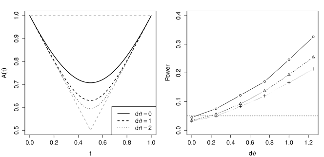
The right plot of Figure 1 displays the rejection rates of the three tests estimated from 2000 samples of size generated under such that, for each sample, the first (resp. last) 50 observations were drawn from c.d.f. (4.6) with (resp. ). As expected, the test based on is more powerful than its two competitors in this simple setting.
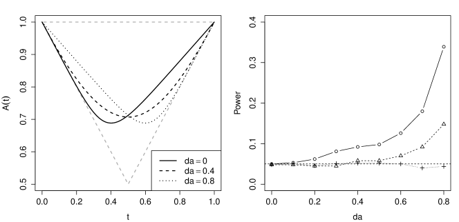
To investigate the influence of asymmetry on the power of the three tests, as a second experiment, we considered again the copula in (4.6), but this time with parameter defined as , for , and with parameter set to keep Kendall’s tau of equal to . The corresponding Pickands dependence functions for are represented in the left plot of Figure 2. The right plot displays the rejection rates of the tests based on , and versus estimated from 2000 samples of size such that, for each sample, the first (resp. last) 100 observations were drawn from the above mentioned copula with (resp. ). Although the rejection rates are overall relatively low, the test based is by far the best. The fact that the test based on has no power against such alternatives is due to the fact that Spearman’s remains almost constant.
| 5 | 50 | 0 | 5.5 | 6.2 | 6.0 | 5.5 | 6.3 | 6.2 |
|---|---|---|---|---|---|---|---|---|
| 0.25 | 6.6 | 6.1 | 6.2 | 5.2 | 4.1 | 3.7 | ||
| 0.5 | 4.3 | 3.3 | 2.5 | 4.4 | 2.8 | 2.7 | ||
| 0.75 | 3.9 | 2.2 | 1.2 | 2.7 | 2.5 | 1.1 | ||
| 100 | 0 | 5.1 | 5.1 | 5.4 | 5.0 | 5.9 | 6.0 | |
| 0.25 | 5.1 | 3.6 | 5.1 | 6.7 | 4.0 | 4.9 | ||
| 0.5 | 5.5 | 4.1 | 4.3 | 4.7 | 2.9 | 3.3 | ||
| 0.75 | 3.3 | 1.0 | 0.6 | 4.5 | 2.8 | 1.5 | ||
| 200 | 0 | 5.6 | 4.8 | 5.5 | 5.6 | 5.8 | 5.4 | |
| 0.25 | 4.8 | 5.1 | 5.1 | 3.9 | 3.6 | 3.4 | ||
| 0.5 | 4.6 | 2.5 | 2.9 | 5.2 | 3.4 | 4.0 | ||
| 0.75 | 4.0 | 0.8 | 1.0 | 5.0 | 3.0 | 2.1 | ||
| 15 | 50 | 0 | 4.5 | 5.6 | 5.3 | 4.7 | 5.3 | 5.3 |
| 0.25 | 7.6 | 5.7 | 5.0 | 6.8 | 6.5 | 6.8 | ||
| 0.5 | 5.2 | 2.8 | 2.1 | 8.6 | 6.7 | 5.3 | ||
| 0.75 | 18.3 | 1.5 | 0.3 | 20.0 | 15.9 | 4.6 | ||
| 100 | 0 | 4.3 | 4.4 | 4.9 | 4.2 | 4.2 | 4.6 | |
| 0.25 | 4.7 | 3.4 | 3.9 | 5.9 | 4.3 | 4.9 | ||
| 0.5 | 7.2 | 3.8 | 3.0 | 9.0 | 8.4 | 6.5 | ||
| 0.75 | 40.6 | 10.0 | 1.8 | 42.0 | 36.9 | 23.0 | ||
| 200 | 0 | 4.3 | 3.8 | 5.4 | 4.2 | 4.3 | 4.3 | |
| 0.25 | 6.4 | 5.5 | 5.2 | 7.7 | 5.5 | 6.5 | ||
| 0.5 | 9.3 | 7.4 | 6.3 | 14.1 | 15.7 | 14.7 | ||
| 0.75 | 75.2 | 56.5 | 36.8 | 79.2 | 79.3 | 71.5 | ||
Empirical power of the tests based on , and under an abrupt change in one margin only
Table 2 reports rejection rates of estimated from 1000 bivariate samples of size generated under where and are defined in (1.3) and (4.1), respectively, such that, for each sample, the first (resp. last ) observations were drawn from a c.d.f. whose copula is the Gumbel–Hougaard, whose first margin is GEV with parameters , and (resp. , and ), and whose second margin is standard normal (the results are unaffected by the choice of the second margin since the test is rank-based).
All three tests have little power against such alternatives when the shift in the location parameter of the first margin is relatively small (). This is a desirable property since the tests were designed to be sensitive to departures from . Higher rejection rates were obtained for and when the dependence is moderate or high, in particular if the (scaled) change-point in the first margin is non-central . The latter results illustrate the fact that the procedures based on , and are tests for and that one should not use them to reject unless holds. Additional changes in the dispersion or scale parameter of the first margin might even increase the phenomenon.
Empirical levels of the test based on
A consequence of Proposition 4.2 is that the test based on will hold its level asymptotically under one abrupt marginal change only, such as those considered in the previous experiment. To evaluate the corresponding finite-sample behavior, we considered again the setting of Table 1. Indeed, because of the rank-based nature of the test based on , samples generated under can equivalently be regarded as generated from . From the last two columns of Table 1, we see that the test based on holds its level equally well as the test based on . The test based on is however slightly too liberal for , although the agreement of its empirical levels with the 5% nominal level improves as increases.
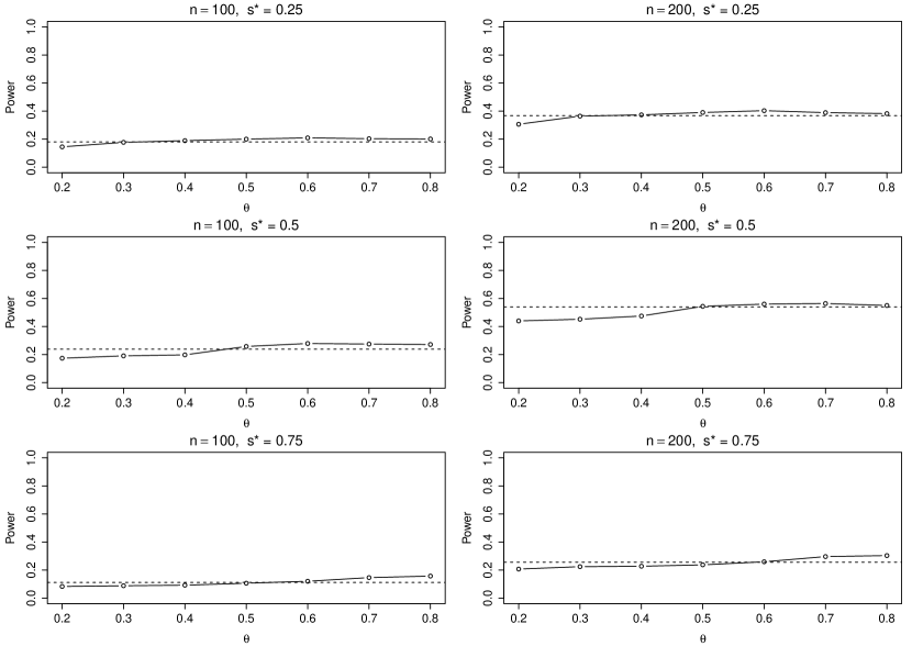
Empirical power of the test based on
As a last experiment, we investigated the influence of the value on the power of the test based on . Figure 3 displays the rejection rates of the test based on against estimated from 1000 bivariate samples of size , such that, for each sample, the first (resp. last ) observations are generated from a Gumbel–Hougaard copula with parameter 2 (resp. 3). The values 0.25, 0.5 and 0.75 were considered for . As one can see, the rejections rates are not too much affected by the value of . In addition, the power of the test based on remains overall reasonably close to that of the test based on . From a practical perspective, the latter result suggests that, under in (1.2), the somehow “non optimal” use of the test based on instead that based on does not incur a large power loss, if any. As a consequence, if one hesitates about which of in (1.2) or in (4.1) holds, it seems safer to use the test based on as, should be actually true, the latter test is more likely to hold its level by construction, and should be true, the power loss, if any, should not be too large.
6 Illustrations
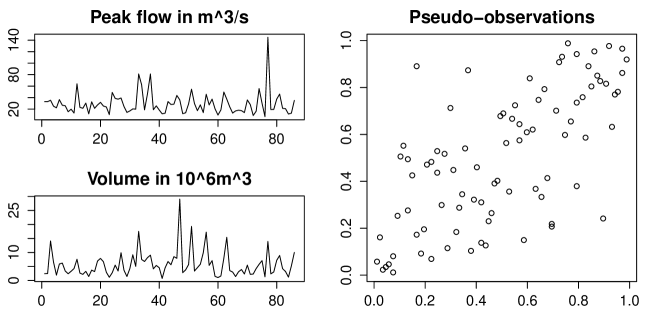
To illustrate the proposed tests, we consider two hydrological data sets. The first one consists of bivariate annual maxima measured between 1921 and 2011 (five years of data are missing) at a station located on the river Preßnitz in Streckewalde, Germany. The variables of interest are , the annual maximal peak flow (in ), and , the annual maximal volume of discharge (in ). Their observations are represented in Figure 4. The joint distribution of and is of strong interest to hydrologists as it can be used to assess the risk of catastrophic flood levels. For a recent case study, we refer to Mitková and Halmová (2014).
Because we are dealing with bivariate block maxima, it is natural to assume that the data arise from one or more bivariate extreme-value distributions. The aim of our analysis is to test for possible changes in the dependence between and that might have occurred during the long period of observation. An additional element to be taken into account here is that a dam was built on the river Preßnitz in 1973 (which corresponds to the th observation) a few kilometers upstream from the measurement station. We make the hypothesis that, if there are changes in the two components series, then, they are unique and they occurred simultaneously after observation 48 due to the construction of the dam. In other words, we assume that either in (1.2) holds or in (4.1) with holds. In the former case, it is natural to use the test for change-point detection based on in (3.7), while in the latter case, the extension based on in (4.5) with should be preferred. As mentioned in the previous section (see Figure 3 and the related discussion), using the test based on for some value of when in (1.2) actually holds does not seem to result in a strong power loss, if any. For that reason, we carried out the test based on with . The resulting approximate p-value of 0.068, obtained from multiplier bootstrap replicates, indicates that there is some weak evidence of change in the dependence between and . Interestingly enough, the maximum of the test statistic was not obtained for observation 48 but for observation 32 corresponding to year 1953.
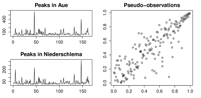
The second data set consists of peak flows (in ) simultaneously measured at two neighboring gauges for physically independent summer flood events. The two gauges are located in Germany, in Aue and Niederschlema, respectively, and the corresponding measurements will thus be denoted by and , respectively. The observations, chronologically ordered, span the period 1929-2011 and are represented in Figure 5. An event was classified as a flood, if each peak flow exceeded the smallest annual maximal peak flow measured between 1929 and 2011 in Aue and Niederschlema, respectively. The period of each flood event was identified by hand and only the largest value (peak flow) was included in the data set. Hence, by construction, the observations are formed subject to a block maximal procedure, with possibly slightly differing block sizes for each of the flood events. It therefore seems sensible to assume that the data-generating distribution(s) are extreme-value distributions.
There were two reasons why only summer events were included in the analysis. First, typical winter floods are produced from melting snow, whereas summer floods are due to short but heavy rainfalls. These very different physical mechanisms lead to different peak flow distributions. Second, very high peak flows, which are of particular interest, almost exclusively occur during the summer time. The joint distribution of peak flows is of interest, for instance, to evaluate the efficiency of water reservoirs (Schulte and Schumann, 2015).
The aim of our analysis is to assess whether the dependence between and changed during the long observation period. As for the previous illustration, it might be important to take into account the fact that dams where constructed on the river Mulde and one of its tributary upstream of the two gauges Aue and Niederschlema. A first dam, called Schönheiderhammer, was put in service in 1980 (which corresponds to observation 108) and a second dam, named Eibenstock, was put into service in 1982. As previously, we make the hypothesis that, if there are changes in the two components series, then, they are unique and they occurred simultaneously after observation 108 due to the construction of the dams. Following the same reasoning as for the first illustration, we apply the test based on in (4.5) with and obtain an approximate p-value of 0.195 based on multiplier bootstrap replicates. Hence, there is no evidence for a change in the dependence between and .
Appendix A Proofs of Propositions 3.1, 3.2 and 4.1
Propositions 3.1 and 3.2 will be corollaries of a more general result. Recall that and let for . Also, consider the process
| (A.1) |
where is defined in (3.5), and note that
| (A.2) |
is the process of interest in Proposition 3.1.
Theorem A.1.
Under the conditions of Proposition 3.2, in the normed space , we have , where
| (A.3) |
Proof.
Since for , we can write, for ,
where denotes the empirical copula, see (3.11). Similarly, for ,
Therefore, introducing the notation
we obtain, for any such that ,
| (A.4) |
where, for any ,
denotes the two-sided sequential empirical copula process studied in Bücher and Kojadinovic (2014). Since is continuously differentiable on , we have, from Example 5.3 in Segers (2012), that the first-order partial derivatives and of exist and are continuous on and , respectively. Hence, from Theorem 3.4 in Bücher and Kojadinovic (2014),
| (A.5) |
where, for any ,
| (A.6) |
with the convention that if , and where
with , . From (A.5), the fact that in under (see, e.g., van der Vaart and Wellner, 1996, Theorem 2.12.1), the fact that and and the continuous mapping theorem, it follows that the process
| (A.7) |
weakly converges in to in (A.3). The theorem is thus proved if we show that
| (A.8) |
For that purpose, let us first show that, for any with and any ,
| (A.9) |
First of all, we have, for any and any ,
The number of is , and of those, exactly do not exceed . The same is true for the . Hence, for at least
of the pairs, both pseudo-observations do not exceed . As a consequence,
In particular, we have for all such that . Since , we get that
| (A.10) |
Together with the fact that , the last display implies the bound in (A.9).
In order to prove (A.8), notice first that, by (A), (A.7), the triangle inequality and (A.9),
both sides of the inequality being zero if the suprema are restricted to such that . Next, fix . Using the fact that that vanishes when and that is asymptotically uniformly equicontinuous in probability, there exists such that, for all sufficiently large ,
The proof of (A.8) will thus be complete if we show that
which, in view of (A.9), would be an immediate consequence of the fact that
Using again the identity , the last display follows from the fact that
which completes the proof. ∎
Proof of Proposition 3.2..
The assertion is a mere consequence of the fact that, under ,
| (A.11) |
Theorem A.1, and the continuous mapping theorem. ∎
Lemma A.2.
Under and if is continuously differentiable on ,
Proof.
Both suprema are measurable, and they are equal in distribution to the same suprema calculated under . The assertions then follow from (A.5). ∎
Proof of Proposition 4.1.
Let
| (A.12) |
where is defined in (4.3). We shall first show that
| (A.13) |
and that
| (A.14) |
where is defined in (A.7). Proceeding as in (A), for , we have
Using the fact that for all , the supremum on the left of (A.13) is smaller than , where
and
From Lemma A.2, the weak convergence of in under , and the continuous mapping theorem, . Concerning , by the definition of in (4.2), we have that
Hence, in , which, from the continuous mapping theorem, implies that . This completes the proof of (A.13). The proof of (A.14) is similar.
To finish the proof, notice first that, under ,
where is defined in (A.12). Next, let
where and denote the minimum and maximum operators, respectively,
| (A.15) |
and is defined in (A.6), and let
The desired result shall then follow from the fact that
| (A.16) | |||
| (A.17) |
and
| (A.18) |
where is given in (3.9). To show that (A.16) holds, it suffices to restrict the supremum in (A.16) successively to and and use the triangle inequality, (A.8), and (A.13) and (A.14), respectively. The fact that (A.17) holds is obtained from the triangle inequality and Lemma A.2. Finally, (A.18) follows from the fact that, for any , , the weak convergence of under and the continuous mapping theorem. ∎
Appendix B Proofs of Propositions 3.3 and 4.2
Just as for the non-bootstrap results in Propositions 3.1 and 3.2, Propositions 3.3 and 4.2 can be conveniently proved using appropriate two-sided sequential processes. For and , let
| (B.1) |
and
| (B.2) |
Next, for and , let
and
Furthermore, from (2.2), for , we obtain that
| (B.3) |
and
| (B.4) |
where is extended by continuity at 0 and 1. Indeed, from the fact that for all , we have that for all , and, from the convexity of on , we have that is increasing on . In addition, we adopt the usual convention that . Finally, for and , let
| (B.5) |
and
| (B.6) |
Lemma B.1.
Proof.
Lemma B.2.
Under and if is continuously differentiable on , for any ,
Proof.
From the proof of Proposition 4.3 of Bücher et al. (2014) (see the term (B.3)), we have that, for ,
where and are defined in (3.10) and (B.1). The desired result will follow if we show that
| (B.7) |
where is defined in (B.2). The supremum on the left of the previous display is smaller than
Using the fact that the first supremum is bounded by 2, the asymptotic uniform equicontinuity in probability of the process (by Donsker’s theorem) which vanishes when , and the weak convergence in , we obtain that the latter display is . Hence, (B.7) holds. ∎
For and for , let
| (B.8) |
where is defined in (3.13). Furthermore, for and , let
| (B.9) | ||||
| (B.10) |
where is defined in (3.14) and with the convention that if . Finally, for and , let
Lemma B.3.
Proof.
Proof of Proposition 3.3..
For and , let
where is defined in (B.5), and let
where is defined in (B.6). From Lemma B.2, we then immediately obtain that
The latter combined with Lemma B.1, the continuous mapping theorem, (A.5), (A.8) and (A.11) gives
in , where is defined in (3.9) and are independent copies of . From the definitions in (3.12) and (B.8), we further have that, for ,
Hence, to complete the proof, it remains to show , which is implied by
| (B.12) |
Having in mind the fact that converges uniformly in probability to as a consequence of Proposition 3.1, (B.7) and the fact and , to prove (B.12), it suffices to show that
| (B.13) |
and
| (B.14) |
where , , and are given in (B.9), (B.10), (B.3) and (B.4), respectively.
From (A.10), it can be verified that, for any and any , . Since, by definition, in (3.14) is also uniformly bounded, and are uniformly bounded.
To prove (B.13), we can then proceed as in the proof of Proposition 4.3 of Bücher et al. (2014) (see the terms (B.4) and (B.5)). Using the asymptotic uniform equicontinuity in probability of which vanishes when , and the fact that and its estimator are uniformly bounded, it remains to show that, for any ,
| (B.15) |
The previous result is implied by the fact that
where is defined in (A.1), and an analogue result for defined in (3.14). The latter can be seen as follows: for in (3.15), we have
| (B.16) |
Since , extended by continuity, is (uniformly) continuous on (see the discussion below (B.4)), by the mean value theorem, the first term on the right converges to zero. The second term on the right is smaller than
by asymptotic uniform equicontinuity in probability of .
Proof of Proposition 4.2.
For , let be the analogue of in (B.8) based on the adapted pseudo-observations defined in (4.4). Then, by definition of , we have
Next, let
where is defined in (B.6), and let us first show that
| (B.17) |
To prove (B.17), we shall show that
| (B.18) |
and
| (B.19) |
We start with the proof of (B.18). Under , (B.12) continues to hold if the supremum is restricted to . This can be seen by essentially the same arguments as in the proof of Lemma A.2. Therefore, (B.18) will hold if
that is, if
| (B.20) |
and, having in addition (B.3), (B.4), (B.9) and (B.10) in mind, if
| (B.21) | |||
| (B.22) |
where is the analogue of in (3.14) defined from the adapted pseudo-observations in (4.4). The supremum on the left of (B.20) is smaller than
by Lemma A.2 and the weak convergence of under . The supremum on the left of (B.21) is smaller than
where is defined in (A.12), and is because of (A.13), (A.7), Lemma A.2 and the weak convergence of under . The proof of (B.22) is based on a decomposition similar to that used in (B.16) and relies again on (A.13). Hence, (B.18) holds. The proof of (B.19) is similar.
Using arguments of the same nature as those employed in the proof of Lemma A.2, we obtain the following extension of Lemma B.2 under :
By the triangular inequality, this implies that
| (B.23) |
where
and is defined in (B.5). The desired result is then a consequence of Lemma B.1, the continuous mapping theorem, (A.16), (A.17), (B.17) and (B.23). ∎
Appendix C Test statistic and multiplier bootstrap for
In Sections 3 and 4, we restricted ourselves to the case . Results for arbitrary dimension can be established at the cost of a more complex notation but without significant additional mathematical difficulties. We give the main steps of the generalization hereafter. Let be a random vector with c.d.f. and extreme-value copula of the form (2.1) and (2.2), respectively, and suppose that is continuously differentiable on the interior of with partial derivatives , . With the notation , , and , , we have, just as for ,
with the convention that for all .
Let , , be independent copies of and let be -variate generalizations of the “subsample” pseudo-observations in (3.4). We define a CUSUM-type process on by
where, for , , and
with the convention that if .
Let us introduce some additional notation. For any and , we define to be the vector with the convention that . Furthermore, for any and any , denotes the vector of whose components are all equal to one, except the th which is equal to .
Proposition C.1.
Suppose that all of the above conditions are met. Then, in the normed space , , where
Here, denotes a centered Gaussian process on defined through
where is a tight, centered Gaussian process on with covariance kernel given by
and , , denotes the th first-order partial derivative of .
The proof is almost identical to that of Proposition 3.2. For a corresponding bootstrap approximation of the limit , let , , be i.i.d. standard normal multipliers. Furthermore, from (2.2), we have that, for any and ,
The above quantities can be estimated consistently by plugging in subsample estimators of and , , respectively, namely and
with and a sequence such that (boundary effects can be dealt with by generalizing the approach adopted below (3.15)). Then, analogously to the bivariate case, we define
where, for ,
with and denoting the arithmetic mean over of
and where
Test statistics and corresponding multiplier bootstrap replicates can be defined analogously to Section 3, as functionals of and , , respectively. In addition, generalizations adapted to known breaks in the margins can be obtained by computing pseudo-observations from the subsamples determined by the marginal change-points, as explained in Section 4. We omit the details for the sake of brevity.
Acknowledgements. The authors would like to thank Markus Schulte and Andreas Schumann for providing us with the hydrological data sets and Betina Berghaus and Roland Fried for helpful discussions. This work has been supported by the Collaborative Research Center “Statistical modeling of nonlinear dynamic processes” (SFB 823) of the German Research Foundation (DFG) which is gratefully acknowledged.
References
- Aue and Horváth (2013) Aue, A. and L. Horváth (2013). Structural breaks in time series. J. Time Series Anal. 34(1), 1–16.
- Beirlant et al. (2004) Beirlant, J., Y. Goegebeur, J. Segers, and J. Teugels (2004). Statistics of extremes: Theory and Applications. Wiley Series in Probability and Statistics. Chichester: John Wiley & Sons Ltd.
- Bücher and Kojadinovic (2014) Bücher, A. and I. Kojadinovic (2014). A dependent multiplier bootstrap for the sequential empirical copula process under strong mixing. Bernoulli (to appear), arXiv:1306.3930.
- Bücher et al. (2014) Bücher, A., I. Kojadinovic, T. Rohmer, and J. Segers (2014). Detecting changes in cross-sectional dependence in multivariate time series. J. Multivariate Anal. 132(0), 111 – 128.
- Bücher and Segers (2014) Bücher, A. and J. Segers (2014). Extreme value copula estimation based on block maxima of a multivariate stationary time series. Extremes 17(3), 495–528.
- Cooley et al. (2007) Cooley, D., D. Nychka, and P. Naveau (2007). Bayesian spatial modeling of extreme precipitation return levels. Journal of the American Statistical Association 102(479), 824–840.
- Csörgő and Horváth (1997) Csörgő, M. and L. Horváth (1997). Limit theorems in change-point analysis. Wiley Series in Probability and Statistics. Chichester, UK: John Wiley & Sons.
- de Haan and Ferreira (2006) de Haan, L. and A. Ferreira (2006). Extreme value theory: an introduction. Springer.
- Dümbgen (1991) Dümbgen, L. (1991). The asymptotic behavior of some nonparametric change-point estimators. Annals of Statistics 19(3), 1471–1495.
- Ferreira (2013) Ferreira, M. (2013). Nonparametric estimation of the tail dependence coefficient. REVSTAT – Statistical Journal 11(1), 1–16.
- Genest et al. (1998) Genest, C., K. Ghoudi, and L.-P. Rivest (1998). Discussion of “Understanding relationships using copulas”, by E. Frees and E. Valdez. North American Actuarial Journal 3, 143–149.
- Genest et al. (2011) Genest, C., I. Kojadinovic, J. Nešlehová, and J. Yan (2011). A goodness-of-fit test for bivariate extreme-value copulas. Bernoulli 17(1), 253–275.
- Genest and Segers (2010) Genest, C. and J. Segers (2010). On the covariance of the asymptotic empirical copula process. J. Multivariate Anal. 101(8), 1837–1845.
- Gumbel (1958) Gumbel, E. J. (1958). Statistics of extremes. New York: Columbia University Press.
- Hofert et al. (2015) Hofert, M., I. Kojadinovic, M. Mächler, and J. Yan (2015). copula: Multivariate dependence with copulas. R package version 0.999-13.
- Hosking and Wallis (2005) Hosking, J. R. M. and J. R. Wallis (2005). Regional frequency analysis: an approach based on L-moments. Cambridge University Press.
- Jaruškova and Rencová (2008) Jaruškova, D. and M. Rencová (2008). Analysis of annual maximal and minimal temperatures for some European cities by change point methods. Environmetrics 19, 221–233.
- Katz and Brown (1992) Katz, R. and B. Brown (1992). Extreme events in a changing climate: Variability is more important than averages. Climatic Change 21(3), 289–302.
- Khoudraji (1995) Khoudraji, A. (1995). Contributions à l’étude des copules et à la modélisation des valeurs extrêmes bivariées. Ph. D. thesis, Université Laval, Québec, Canada.
- Kojadinovic (2014) Kojadinovic, I. (2014). npcp: Some nonparametric tests for change-point detection in (multivariate) observations. R package version 0.1-1.
- Kojadinovic et al. (2015) Kojadinovic, I., J.-F. Quessy, and T. Rohmer (2015). Testing the constancy of Spearman’s rho in multivariate time series. Annals of the Institute of Statistical Mathematics, in press.
- Liebscher (2008) Liebscher, E. (2008). Construction of asymmetric multivariate copulas. Journal of Multivariate Analysis 99, 2234–2250.
- Mitková and Halmová (2014) Mitková, V. B. and D. Halmová (2014). Joint modeling of flood peak discharges, volume and duration: a case study of the danube river in bratislava. Journal of Hydrology and Hydromechanics 62(3), 186–196.
- Nelsen (2006) Nelsen, R. B. (2006). An introduction to copulas (Second ed.). Springer Series in Statistics. New York: Springer.
- Pickands (1981) Pickands, III, J. (1981). Multivariate extreme value distributions. In Proceedings of the 43rd session of the International Statistical Institute, Vol. 2 (Buenos Aires, 1981), Volume 49, pp. 859–878, 894–902. With a discussion.
- R Core Team (2015) R Core Team (2015). R: A Language and Environment for Statistical Computing. Vienna, Austria: R Foundation for Statistical Computing.
- Rémillard and Scaillet (2009) Rémillard, B. and O. Scaillet (2009). Testing for equality between two copulas. J. Multivariate Anal. 100(3), 377–386.
- Ressel (2013) Ressel, P. (2013). Homogeneous distributions – And a spectral representation of classical mean values and stable tail dependence functions. Journal of Multivariate Analysis 117, 246–256.
- Scaillet (2005) Scaillet, O. (2005). A Kolmogorov-Smirnov type test for positive quadrant dependence. Canad. J. Statist. 33(3), 415–427.
- Schulte and Schumann (2015) Schulte, M. and A. Schumann (2015). Downstream-directed performance assessment of reservoirs in multi-tributary catchments by application of multivariate statistics. Water Resources Management 29(2), 419–430.
- Segers (2012) Segers, J. (2012). Asymptotics of empirical copula processes under non-restrictive smoothness assumptions. Bernoulli 18(3), 764–782.
- Sklar (1959) Sklar, A. (1959). Fonctions de répartition à dimensions et leurs marges. Publ. Inst. Statist. Univ. Paris 8, 229–231.
- van der Vaart and Wellner (1996) van der Vaart, A. W. and J. A. Wellner (1996). Weak Convergence and Empirical Processes - Springer Series in Statistics. New York: Springer.
- Yue et al. (1999) Yue, S., T. Ouarda, B. Bobée, P. Legendre, and P. Bruneau (1999). The gumbel mixed model for flood frequency analysis. Journal of Hydrology 226(1–2), 88 – 100.