Selective excitation of plasmons superlocalized
at sharp perturbations of metal nanoparticles

Abstract

Sharp metal corners and tips support plasmons localized on the scale of the curvature radius – superlocalized plasmons. We analyze plasmonic properties of nanoparticles with small and sharp corner- and tip-shaped surface perturbations in terms of hybridization of the superlocalized plasmons, which frequencies are determined by the perturbations shape, and the ordinary plasmons localized on the whole particle. When the frequency of a superlocalized plasmon gets close to that of the ordinary plasmon, their strong hybridization occurs and facilitates excitation of an optical hot-spot near the corresponding perturbation apex. The particle is then employed as a nano-antenna that selectively couples the free-space light to the nanoscale vicinity of the apex providing precise local light enhancement by several orders of magnitude.

I Introduction

Efficient coupling of light to nanometer size volumes is one of the biggest challenges of modern optics; it is desired for numerous potential applications. To overcome the light diffraction limit, localized plasmons (LPs) supported by metal nanoparticles and nanowires can be utilized.Novotny07 ; Klimov11 ; Schuller10 In this way, valuable progress has been achieved in creating plasmonic optical sensors of single atoms and molecules,Gissen11 bio-sensors,Brolo and nano-lasers.S1 The related local concentration of light fields strongly enhances the Raman scatteringSERS and the harmonic generation.SHG

Plasmonic properties of a metal nanoparticle are primarily determined by its shape.Novotny07 ; Klimov11 With analytical solutions available only for the simplest (e.g., spherical and ellipsoidal) shapes, many efforts have been spent on numerical modeling of LPs of complex-shape particles.Ruppin ; Kottmann1 ; Kottmann2 ; Kelly03 ; Gonzalez07 ; Prodan ; Hao ; PRB13 ; EPL13 ; JOSAB12 ; PRB14 ; Klimov2014 ; JOSAB14 It is recognized that adding new shape features enriches the LP spectrum considerably. In certain cases, it is possible to consider plasmons of complex particles as a result of hybridization of plasmons supported by constituents of simpler shapeProdan ; Hao similarly to hybridized diatomic electronic states.Landau3

Metal nanoparticles and nanowires with sharp shape features, such as corners and tips, represent an important special case. Perfectly sharp corners and tips are physically meaningless with regard to plasmons.PRB13 The simplest polyhedral 2D particles – wires of smoothed square, triangular and rhomboidal cross sections – exhibit highly specific plasmonic properties: The resonant values of the metal permittivity are determined by the geometric parameters of the corners – the apex angle and the curvature radius.EPL13 ; PRB13 A similar behavior was predicted for 3D particles of smoothed cubic shapes.Klimov2014 Generally, as the sharpness increases, the plasmons become superlocalized, i.e. localized on the scale of the curvature radius. The local values of electric field then exceed considerably those in the incident light wave. Solid links between such superlocalized plasmons (SLPs) of metal corners and tips and the optical singularity at perfectly sharp wedges and cones have been established.PRB14 ; JOSAB14

Nanosize perturbations of metal surface, both randomZhao2014 and regular,JOSAB12 strongly affect plasmons and their contribution to optical phenomena. Sharp perturbations of a flat metal surface also support SLPs which admit a relatively simple analysis including determination of plasmonic frequencies and field distributions.JOSAB14 One can expect that a sharp perturbation provides almost the same SLP properties whether it is placed on the flat metal surface or on a smooth nanoparticle surface. However, this expectation comes true only partially and its failure is worthy of attention. The point is that the frequencies of SLPs and LPs depend on essentially different shape parameters, and for this reason they can eventually be close to each other. In this case, a strong hybridization of large-scale LPs with short-shale SLPs of a nanoparticle can be anticipated.

In this paper, we analyze the SLP-LP hybridization and its optical consequences for the simplest unperturbed nanoparticle shapes with non-degenerate LP spectra (elliptic wires and spherical particles) and sharp corner- and tip-shaped surface perturbations.

II Basic relations

For subwavelength particles, the full set of Maxwell’s equations reduces in the quasi-static approximation to the Laplace equation for the electric potential $\phi$ .Novotny07 ; Klimov11 The latter satisfies the conventional boundary conditions including the relative (to the dielectric background) complex permittivity $\varepsilon(\omega)=\varepsilon^{\prime}(\omega)+i\varepsilon^{\prime\prime}(\omega)$. Furthermore, it is convenient to transfer from the differential eigenvalue problem for $\phi$ in space to an equivalent integral problem for the surface charge density $\sigma$.Klimov11 ; PhilMag89 ; Mayergoyz05 In this approach, the plasmonic eigenfunctions $\sigma_{j}$ obey the integral equation

$$\int_{B}K({\bf r},{\bf r}^{\prime})\,\sigma_{j}({\bf r}^{\prime})d{\bf r}^{\prime}=\Lambda_{j}\,\sigma_{j}({\bf r}),$$ (1)

where the eigenvalues $\Lambda_{j}=(\varepsilon_{j}+1)/(\varepsilon_{j}-1)$ are expressed by the real resonant permittivity $\varepsilon_{j}$, the kernels in the 3D case (nanoparticle) and the 2D case (nanowire) are

$$K_{\rm 3D}({\bf r},{\bf r}^{\prime})=\frac{{\bf n}\cdot({\bf r}-{\bf r}^{\prime})}{2\pi\,|{\bf r}-{\bf r}^{\prime}|^{3}},\ K_{\rm 2D}({\bf r},{\bf r}^{\prime})=\frac{{\bf n}\cdot({\bf r}-{\bf r}^{\prime})}{\pi\,|{\bf r}-{\bf r}^{\prime}|^{2}},$$ (2)

$B$ is the 3D or 2D boundary of the particle, and ${\bf n}={\bf n}({\bf r})$ is the unit vector of the external normal.

Although the integral operator in Eq. (1) is non-symmetric, its eigenvalues are real and its eigenfunctions are mutually orthogonal for the scalar product defined as Klimov11 ; PhilMag89

$$(\sigma_{1}\cdot\sigma_{2})_{\rm 3D}=\int_{B}\ \frac{\sigma_{1}({\bf r})\sigma_{2}({\bf r}^{\prime})}{|{\bf r}-{\bf r}^{\prime}|}d{\bf r}^{\prime}d{\bf r},$$ (3)

$$(\sigma_{1}\cdot\sigma_{2})_{\rm 2D}=-2\int_{B}\sigma_{1}({\bf r})\sigma_{2}({\bf r}^{\prime})\ln(|{\bf r}-{\bf r}^{\prime}|)d{\bf r}^{\prime}d{\bf r}.$$ (4)

This allows us to normalize $\sigma_{j}$ as $(\sigma_{j}\cdot\sigma_{k})=\int_{B}\sigma_{j}\phi_{k}d{\bf r}^{\prime}\equiv\langle\sigma_{j}\phi_{k}\rangle=\delta_{jk}$, where $\phi_{k}({\bf r})$ is the surface value of the electric potential induced by the charge density $\sigma_{k}$ and the brackets denote the surface integral. Note that $\phi_{k}$ can be also obtained directly as a solution (denoted as $\tau_{k}$ in Ref. Mayergoyz05, ) of the integral problems adjoint to Eq. (1), i.e., with the arguments of the kernels permuted.

Considering the particle in an external electric field ${\bf E}_{0}(\bf r)$, one can find the coefficients of expansion of $\sigma$ in terms of $\sigma_{j}$ and calculate the key observables.Klimov11 ; Mayergoyz05 ; PRB13 In particular, evaluation of the induced dipole moment of the particle $\langle{\bf r}\sigma\rangle$ yields the polarizability tensor

$$\alpha_{\mu\nu}=\sum\limits_{j}\frac{[\varepsilon(\omega)-1](\varepsilon_{j}-1)}{4\pi[\varepsilon_{j}-\varepsilon(\omega)]}{\langle r_{\mu}\sigma_{j}\rangle\langle\phi_{j}n_{\nu}\rangle},$$ (5)

where $r_{\mu}$ and $n_{\nu}$ are components of $\bf r$ and $\bf n$. One can also calculate the normal component of the total electric field above the particle surface and determine its ratio to the external field applied in the same direction:

$$\xi({\bf r})=1+\sum\limits_{j}\frac{\varepsilon_{j}[\varepsilon(\omega)-1]}{\varepsilon_{j}-\varepsilon(\omega)}\langle\phi_{j}({\bf r}^{\prime})\ {\bf n}({\bf r}^{\prime})\cdot{\bf n}({\bf r})\rangle\ \sigma_{j}({\bf r}).$$ (6)

The absolute value $|\xi|({\bf r})$ gives the local light-field enhancement factor.

Note the presence of the complex-valued factors $[\varepsilon_{j}-\varepsilon(\omega)]$ in the denominators of Eqs. (5) and (6) that reach their minimum absolute values $|\varepsilon^{\prime\prime}(\omega_{j})|$ at the resonant frequencies $\omega_{j}$ such that $\varepsilon^{\prime}(\omega_{j})=\varepsilon_{j}$. Accordingly, a strong resonant increase of the particle response can be expected if $\varepsilon^{\prime\prime}(\omega_{j})\ll|\varepsilon^{\prime}(\omega_{j})|$. Often it is sufficient to restrict ourselves to a single resonant term in Eqs. (5) and (6).

Numerical solution of the eigenvalue problem (1) is the most demanding stage of calculations. In the 2D case, it poses a one-dimensional integral eigenvalue problem which can be solved on a desktop computer. In the 3D case, it can be considerably simplified by choosing appropriate particular cases, e.g., by considering a particle of axially symmetric shape that allows surface parametrization in the spherical coordinates as a single-valued function $r=r(\theta)$. Then one can introduce the charge density $\sigma(\theta,\varphi)$ and search for the eigenfunctions in the form $e^{im\varphi}\sigma_{j}(\theta)$ with integer $m$. For the external electric field applied along the symmetry axis, only the modes with $m=0$ are excited, and Eq. (1) leads to a 1D integral eigenvalue problem.

III Numerical results

III.1 Sharp corner on wire

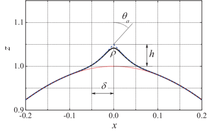
Figure 1: Profile of the corner-shaped perturbation of elliptical wire as described by Eqs. (7) and (8) for $a=2$, $\delta=0.05$, $h=0.05$, and $\rho=0.01$ (solid line). The dotted and dashed lines show the unperturbed wire and ideally sharp $\rho\rightarrow 0$ perturbation profiles respectively.

Let us consider a wire of elliptical cross-section with a sharp corner-shaped perturbation. The ellipticity removes the frequency degeneracy of LPs of a circular wire. The scale invariance allows for an arbitrary size normalization, and we parameterize the unperturbed wire boundary line in the polar coordinates as

$$r_{0}(\varphi)=(\cos^{2}\varphi+a^{2}\sin^{2}\varphi)^{-1/2},$$ (7)

where $a$ is the ellipse axis ratio. The perturbed boundary line $r(\varphi)=r_{0}(\varphi)+r_{1}(\varphi)$ includes a small sharp corner-shaped perturbation given by

$$r_{1}(\varphi)=\frac{h\delta\ e^{-\varphi^{2}/\delta^{2}}}{\sqrt{\delta^{2}+\varphi^{2}}+\sqrt{p^{2}+\varphi^{2}}},$$ (8)

where the height $h$ and the half-width $\delta$ are small positive parameters, the half apex angle of the corner is $\theta_{a}=\arctan(\delta/h)$, and the sharpness is controlled by the small parameter $p$ that determines the curvature radius $\rho=p\delta/h$, see Fig. 1.

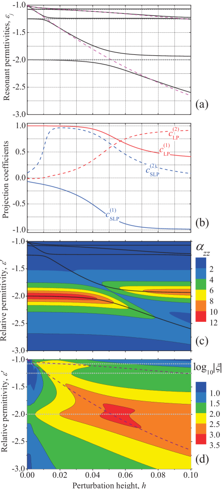
Figure 2: Plasmonic properties of elliptic wire (the axis ratio $a=2$) with the corner-shaped perturbation of the half-width $\delta=0.05$, the curvature radius $\rho=0.01$ and variable height $h$. (a): The lowest resonant permittivity branches (solid) compared to those for the same perturbation of plane surface JOSAB14 (dashed) and those of the unperturbed wire (dotted). (b): Projection coefficients for the plasmons with the lowest (solid) and second-lowest (dashed) resonant permittivities.(c): Color map of the wire polarizability with the resonant permittivity branches shown by lines. (d): Color map of the field enhancement factor with the SLP- and LP-branches shown by dashed and dotted lines respectively. The ratio $|\varepsilon^{\prime}|/\varepsilon^{\prime\prime}=20$ was assumed for (c) and (d).

With this parametrization we solved numerically Eq. (1) using a discretization with crowding of points near the corner apex. The typical number of points about $1000$ was sufficient, and it was made sure that the general modal properties – zero total charge, twin symmetry,Mayergoyz05 and orthogonality – were accurately fulfilled.

Four lowest branches $\varepsilon_{j}(h)$ for the perturbed elliptic cross-section are shown in Fig. 2a by solid lines. The intersecting horizontal dotted lines and negatively tilted dashed lines, given for comparison, show a few lowest resonant permittivity branches for the unperturbed wire (LP-branches) and for the same sharp perturbation placed on flat surfaceJOSAB14 (SLP-branches), respectively. Each $\varepsilon_{j}(h)$ branch stays close either to an LP-branch or to an SLP-branch except for the vicinities of their intersections. Evidently, in these regions we have a strong hybridization of localized and superlocalized plasmons with the avoided crossing structure of the branches typical for hybridized states.Landau3

Furthermore, we have found that the surface-charge distributions $\sigma_{j}(\varphi)$ are close to superpositions of $\sigma_{\rm LP}(\varphi)$ and $\sigma_{\rm SLP}(\varphi)$ corresponding to the LP resonances of the unperturbed wire and the SLP resonances of the perturbation placed on a flat surface:

$$\sigma_{j}\approx c^{(j)}_{\rm LP}\sigma_{\rm LP}+c^{(j)}_{\rm SLP}\sigma_{\rm SLP}.$$ (9)

The mixing coefficients can be evaluated as projections $c^{(j)}_{\rm LP}=(\sigma_{j}\cdot\sigma_{\rm LP})$ and $c^{(j)}_{\rm SLP}=(\sigma_{j}\cdot\sigma_{\rm SLP})$. As seen from Fig. 2b, the surface charge distributions are very close either to $\sigma_{\rm LP}$ (when $|c^{(j)}_{\rm LP}|\approx 1$ and $|c^{(j)}_{\rm SLP}|\ll 1$) or to $\sigma_{\rm SLP}$ (when $|c^{(j)}_{\rm SLP}|\approx 1$ and $|c^{(j)}_{\rm LP}|\ll 1$) when the $\varepsilon_{j}$ branches are close to LP- and SLP-branches respectively.

Near the avoided crossings, the LP and SLP contributions to $\sigma_{j}$ are comparable. Here the wire optical properties – the polarizability and the field enhancement factor – behave very peculiarly. A representative color map of the polarizability in Fig. 2c shows that a noticeable dipole response of the wire occurring only when the relative permittivity is close to that of the lowest LP resonance is suppressed by the perturbation near the avoided crossing. At the same time, the field enhancement factor $|\xi|$ experiences there a dramatic increase by several orders of magnitude (see Fig. 2d).

Figure 3: Plasmonic properties of the spherical particle with the tip-shaped perturbation of the half-width $\delta=0.1$, the curvature radius $\rho=0.01$ and variable height $h$. (a): The lowest resonant permittivity branches (solid) compared to those for the same perturbation of plane surface JOSAB14 (dashed) and those of the unperturbed sphere (dotted). (b): Projection coefficients of the plasmons with the lowest (solid) and second-lowest (dashed) resonant permittivities. (c): Color map of the polarizability with the resonant permittivity branches shown by lines. (d): Color map of the field enhancement factor with the SLP-and LP-branches shown by dashed and dotted lines respectively. The ratio $|\varepsilon^{\prime}|/\varepsilon^{\prime\prime}=20$ was assumed for (c) and (d).

III.2 Sharp tip on spherical particle

In the 3D case, a very similar situation occurs for a small sharp tip-shaped perturbation of a smoothly shaped nanoparticle. As the simplest example we consider a spherical particle with a conical tip of the same cross-section as above, i.e., of the shape obtained by rotating the profile in Fig. 1 around the vertical axis. Accordingly, the particle surface is parameterized in the spherical coordinates by the polar angle dependent radius vector $r(\theta)=r_{0}(\theta)+r_{1}(\theta)$ where the functions $r_{0}$ and $r_{1}$ are given by Eqs. (7) and (8) and $a=1$.

The obtained branches of the resonant permittivity shown in Fig. 3a follow either the horizontal LP-branches of the unperturbed sphere or the tilted SLP-branches of the conical tip on a flat surface. Near the intersections of the LP- and SLP-branches, the avoided crossings indicating strong hybridization occur. We evaluated the projection coefficients $c^{(j)}_{\rm LP}$ and $c^{(j)}_{\rm SLP1,2}$ using the charge distribution $\sigma_{\rm LP}$ of the lowest (dipolar) LP resonance of the unperturbed sphere and distributions $\sigma_{\rm SLP1}$ and $\sigma_{\rm SLP2}$ of the lowest (SLP1) and second-lowest (SLP2) resonances of the tip-shaped perturbation of a flat surface respectively. As illustrated by Fig. 3b, the plasmon charge densities are very close either to $\sigma_{\rm LP}$ or to $\sigma_{\rm SLP1,2}$ and a noticeable LP-SLP mixing occurs near the avoided crossings.

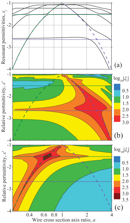
Figure 4: Plasmonic properties of elliptic wire of variable cross section axis ratio $a$ with a pair of corner-shaped perturbations of the same half-width $\delta=0.05$ and curvature radius $\rho=0.01$ and different heights, $h_{1}=0.1$ and $h_{2}=0.025$, located at $\varphi=0$ and $\varphi=\pi/2$ respectively. (a): The lowest resonant permittivity branches (solid) compared to those for the SLPs of the same perturbations of plane surface JOSAB14 (horizontal dotted) and for the LPs of elliptical wire (dashed). (b) and (c): Color maps of the local field enhancement factor on perturbations 1 and 2 respectively; the lowest SLP-branches for the same perturbations on plane surface and the LP-branches of the wire are shown as in (a); $|\varepsilon^{\prime}|/\varepsilon^{\prime\prime}=20$ is assumed.

The colormaps of polarizability and field enhancement factor presented in Figs. 3c and 3d respectively also show qualitative similarity with the 2D-case. Quantitatively, the band of high polarizability here is less affected by the perturbation showing a smaller decrease near the avoided crossings. The difference stems apparently from the weaker LP-SLP interaction in the 3D case (for the same perturbation size) as the tip-shaped perturbation is localized in all directions. Note that the field enhancement factor here is much higher (for the same perturbation curvature radius) and reaches the values of the order of $10^{5}$ near the avoided crossings.

III.3 Two sharp corners on wire

To clarify the situation when two sharp perturbations are present, we consider a wire of elliptical cross section with a well separated pair of corner-shaped perturbations of the form (8). We assume that both perturbations have equal widths and curvature radii but different heights, $h_{1}$ and $h_{2}$, and are located at $\varphi=0$ and $\varphi=\pi/2$ respectively. To demonstrate the sensitivity of the SLP excitation to the unperturbed wire shape, we consider the variable axis ratio $a$.

As seen in Fig. 4a, the resonant permittivity branches here also form avoided crossings near the intersections of the wire LP-branches (the lowest are given by $\varepsilon=a^{\pm 1}$) and the SLP-branches of the perturbations (independent of the wire cross section and represented by the horizontal lines). The local field enhancement at the perturbation apexes increases dramatically near the avoided crossing points as seen in Figs. 4b and 4c. Importantly, the difference in the perturbation height grants a well pronounced spectral isolation of these hot-spots and no interaction between them can be traced from our data.

IV Discussion

As we have seen, each small sharp perturbation of the nanoparticle shape supports plasmons superlocalized near the perturbation apex. Their frequencies are determined by the corresponding perturbation shape. When one of SLP frequencies is close to that of the ordinary LPs (localized on the whole particle) a strong LP-SLP hybridization occurs enabling an LP-SLP synergy. The latter is very beneficial for the light-particle interactions: Large resonant excitation cross-section of LPs is combined with the high local-field concentration in SLPs. As a result, the whole particle plays the role of a nano-antenna that couples free-space light to the nanoscale volume at the top of the perturbation.

When several small sharp perturbations are present, they are generally independent from each other. Accordingly, in real metal nanoparticles with possibly numerous small shape irregularities, only those SLPs will be selectively excited by light whose frequencies are close to the whole particle LP frequencies and only the corresponding perturbations will contribute to optical phenomena.

The conditions of selective SLP excitation are sensitive to the external conditions. By adjusting the background permittivity by 10–20$\%$, one can vary the local-field values by orders of magnitude (see Figs. 2d, 3d, 4b, and 4c). A similar effect can be achieved by changing the close environment, e.g. by displacing the adjacent nanoobjects. This paves the way for targeted design of multi-functional nanoscale optical systems based on metal particles with corner- and tip-shaped features.

The chosen three-scale hierarchy of the particle shape, $\rho\ll\delta\ll 1$, implying smallness of the perturbations and their sharpness, is crucial for our considerations. It ensures the compactness of the hybridization regions (especially in the 3D case) and huge near-field enhancement near the perturbation apexes. Thus, for example, downgrading to a two-scale shape with $\rho=\delta$ results in a dramatic drop of $|\xi|$ by several orders of magnitude. Practically, the chosen scale hierarchy can be realized with the curvature radius of $1$ nm, the corner/tip height and width in the range of $5-10$ nm, and the particle size about $100$ nm. Finally, the assumed ratio $|\varepsilon^{\prime}|/\varepsilon^{\prime\prime}=20$ is a good estimate for silver in the visible, gold in the infrared, and aluminum in the ultraviolet.JC ; Palik ; Rakic

V Conclusion

Plasmon resonances of metal nanoparticles with small sharp shape perturbations are hybrids of plasmons of the two elementary types: the superlocalized plasmons (SLPs) supported of the perturbations and the localized plasmons (LPs) of the unperturbed particles. An efficient optical excitation of an SLP is possible due to a strong LP-SLP hybridization when the SLP frequency is close to an LP frequency. Then the whole particle acts as a nano-antenna that selectively couples the free-space light to a nanoscale optical hot-spot at the top of the corresponding perturbation where the light fields are enhanced by several orders of magnitude.

- (1) L.Nolvotny and B.Hecht, Principles of Nano-Optics, Cambridge University Press (2007).
- (2) V. Klimov, Nanoplasmonics, Pan Stanford Publishing (2011).
- (3) J.A. Schuller, E.S. Barnard, W. Cai, Y.C. Jun, J.S. White, and M.L. Brongersma, Nature Mater. 9, 193 (2010).
- (4) N. Liu, M.L. Tang, M. Hentschel, H. Giessen and A.P. Alivisatos, Nature Mater. 10, 631 (2011).
- (5) A.G. Brolo, Nature Phot.6, 709 (2012).
- (6) D.J. Bergman and M.I. Stockman, Phys. Rev. Lett. 90, 027402 (2003).
- (7) K. Kneipp, M. Moskovits, and H. Kneipp, Electromagnetic Theory of SERS, Springer (2006).
- (8) A. Bouhelier, M. Beversluis, A. Hartschuh, and L. Novotny, Phys. Rev. Lett. 90, 13903 (2003).
- (9) R. Ruppin, Z. Phys. D 36, 69 (1996).
- (10) J.P. Kottmann and O.J.F. Martin, Appl. Phys. B 73, 299 (2001).
- (11) J.P. Kottmann, O.J.F. Martin, D.R. Smith, and S. Schultz, Phys. Rev. B 64, 235402 (2001).
- (12) K.L. Kelly, E. Coronado, L.L. Zhao, and G.C. Schatz, J. Phys. Chem. B 107, 668 (2003).
- (13) A.L. Gonzalez and C. Noguez, J. Computational and Theoretical Nanoscience 4, 231 (2007).
- (14) E. Prodan, C. Radloff, N.J. Halas and P. Nordlander, Science 302, 419 (2003).
- (15) F. Hao, C.L. Nehl , J.H. Hafner and P. Nordlander, Nano Lett. 7, 729 (2007).
- (16) B. Sturman, E. Podivilov, and M. Gorkunov, Phys. Rev. B 87, 115406 (2013).
- (17) B. Sturman, E. Podivilov, and M. Gorkunov, EPL 101, 57009 (2013).
- (18) V. Klimov, G.-Y. Guo, and M. Pikhota, J. Phys. Chem. C 118, 13052 (2013).
- (19) B. Sturman, E. Podivilov, and M. Gorkunov, Phys. Rev. B 89, 045429 (2014).
- (20) B. Sturman, E. Podivilov, and M. Gorkunov, J. Opt. Soc. Am. B 31, 1607 (2014).
- (21) B. Sturman, E. Podivilov, and M. Gorkunov, J. Opt. Soc. Am. B 29, 3248 (2012).
- (22) L.D. Landau and E.M. Lifshits, Quantum mechanics, Pergamon Press, Oxford (1991).
- (23) Y. Zhao, X. Liu, D.Y. Lei , and Y. Chai Nanoscale 6, 1311 (2014).
- (24) F. Ouyang and M. Isaacson Phil. Mag. B 60, 481492 (1989).
- (25) I.D. Mayergoyz, D.R. Fredkin, and Z. Zhang, Phys. Rev. B 72, 155412 (2005).
- (26) P.B. Johnson and R.W. Christy, Phys. Rev. B 6, 4370 (1972).
- (27) D.W. Lynch and W.R. Hunter, in Handbook of Optical Constants of Solids, ed. by E.D. Palik, Academic Press, New York (1985).
- (28) A.D. Rakic, A.B. Djurisic, J.M. Elazar, and M.L. Majewski, Appl. Opt. 37, 5271 (1998).