Recollimation Shocks in Magnetized Relativistic Jets

Abstract

We have performed two-dimensional special-relativistic magnetohydrodynamic simulations of non-equilibrium over-pressured relativistic jets in cylindrical geometry. Multiple stationary recollimation shock and rarefaction structures are produced along the jet by the nonlinear interaction of shocks and rarefaction waves excited at the interface between the jet and the surrounding ambient medium. Although initially the jet is kinematically dominated, we have considered axial, toroidal and helical magnetic fields to investigate the effects of different magnetic-field topologies and strengths on the recollimation structures. We find that an axial field introduces a larger effective gas-pressure and leads to stronger recollimation shocks and rarefactions, resulting in larger flow variations. The jet boost grows quadratically with the initial magnetic field. On the other hand, a toroidal field leads to weaker recollimation shocks and rarefactions, modifying significantly the jet structure after the first recollimation rarefaction and shock. The jet boost decreases systematically. For a helical field, instead, the behaviour depends on the magnetic pitch, with a phenomenology that ranges between the one seen for axial and toroidal magnetic fields, respectively. In general, however, a helical magnetic field yields a more complex shock and rarefaction substructure close to the inlet that significantly modifies the jet structure. The differences in shock structure resulting from different field configurations and strengths may have observable consequences for disturbances propagating through a stationary recollimation shock.

1. Introduction

Very Long Baseline Interferometry (VLBI) observations of Active Galactic Nuclei (AGN) jets often suggests the presence of quasi-stationary features (see, e.g.,  Jorstad et al., 2005; Lister et al., 2013; Cohen et al., 2014). These features can be associated with bends in the jet (see, e.g.,  Alberdi et al., 2000) leading to enhanced emission due to differential Doppler boosting (see, e.g.,  Gómez et al., 1993), or to recollimation shocks (see, e.g.,  Daly & Marscher, 1988; Gómez et al., 1995, 1997; Komissarov & Falle, 1997; Casadio et al., 2013). Most of the observed quasi-stationary features appear in the innermost jet regions (Jorstad et al., 2005, 2013; Fromm et al., 2013; Cohen et al., 2014) suggesting that they could be associated with recollimation, or reconfinement shocks produced by a pressure mismatch between the jet and the external medium.

Multi-wavelength observations of Blazars suggest that high-energy $\gamma$-ray flares are usually associated with the passing of new superluminal components through the VLBI core, defined as the bright compact feature in the upstream end of the jet (see, e.g.,  Marscher et al., 2008, 2010). In order to produce $\gamma$-ray flares, an increase in particle and magnetic energy density is required when jet disturbances cross the radio core. This increase in particle and magnetic density can naturally be explained by identifying the mm-VLBI radio core with a recollimation shock (Gómez et al., 1995, 1997; Marscher et al., 2010; Marscher, 2014). Note however that at centimeter-wavelengths, the opacity core-shift observed in many sources (see, e.g.,  Kovalev et al., 2008; O’Sullivan & Gabuzda, 2008; Sokolovsky et al., 2011) suggests that at these wavelengths the VLBI core corresponds to the transition between the optically thick-thin regimes.

Recollimation shocks have also been found at hundreds of parsecs from the central engine in 3C 120, 3C 380, and M 87 (Roca-Sogorb et al., 2010; Gabuzda et al., 2014; Asada & Nakamura, 2012; Asada et al., 2014). The case of M 87 is particularly interesting since the HST-1 complex, thought associated with a recollimation shock, shows behavior similar to a VLBI core, with new superluminal components emerging from its position (Giroletti et al., 2012). Very high-energy emission has also been observed in connection with variability in the HST-1 region (Cheung et al., 2007) similar to that observed in the VLBI core region of blazars.

When a jet propagates through an ambient medium, pressure mismatch between the jet and the ambient medium naturally arises as a result of ambient pressure decrease. The pressure mismatch drives a radial oscillating motion of the jet and multiple recollimation regions inside the jet (see, e.g.,  Gómez et al., 1997; Komissarov & Falle, 1997; Agudo et al., 2001; Aloy et al., 2003; Roca-Sogorb et al., 2008, 2009; Mimica et al., 2009; Matsumoto et al., 2012). The resulting recollimation structure has been investigated analytically through a self-similar treatment of hydrodynamic jets (Kohler et al., 2012) and magnetized jets (Kohler & Begelman, 2012), while Porth & Komissarov (2014) have studied the causality and stability of magnetized jets propagating in a decreasing pressure ambient medium. If a significant rarefaction wave is produced by the recollimation and propagates into the jet interior, the thermal energy of the plasma can be converted into kinetic energy, increasing considerably the jet Lorentz factor. This is a purely relativistic effect, also referred to as the Aloy-Rezzolla (AR) booster (Aloy & Rezzolla, 2006), which takes place in relativistic flows with a large tangential velocity discontinuity (Rezzolla & Zanotti, 2002). Under these conditions, because the quantity $\gamma h$ is conserved across the rarefaction wave, with $h$ the specific enthalpy and $\gamma$ the Lorentz factor, large jumps can take place in the latter, leading to a boost (Rezzolla & Zanotti, 2013). This boosting mechanism is very basic and has been confirmed by a number of studies in hydrodynamical and magnetized jets (Mizuno et al., 2008; Komissarov et al., 2010; Zenitani et al., 2010; Matsumoto et al., 2012; Sapountzis & Vlahakis, 2013).

In this paper we study in detail how various magnetic field configurations and strength affect the recollimation-shock structure using two-dimensional (2D) special relativistic magnetohydrodynamic (RMHD) simulations. In particular, we focus on the nonlinear rarefactions and shocks excited at the jet and ambient-medium boundary. Our present work provides an extension of the work presented by Gómez et al. (1997) to the case of a dynamically significant magnetic field.

The paper is organized as follows. In Section 2 we describe the numerical method and setup used for our simulations. We present our results in Section 3, illustrating in detail the four different cases of purely hydrodynamical jets, as well as of jets endowed with axial, toroidal and helical magnetic fields. Finally we discuss the astrophysical implications in Section 4, which also contains our conclusions.

2. Numerical Setup

We have perform 2D special-relativistic magnetohydrodynamics (SRMHD) simulations using the three-dimensional general relativistic MHD code RAISHIN adopting cylindrical coordinates ($R$, $\phi$, $z$) (Mizuno et al., 2006, 2011). In particular, we solve the SRMHD equations in the form

$$\partial_{t}\left(\gamma\rho\right) + {1\over R}\partial_{R}\left(R\gamma\rho v^{R}\right)+{1\over R}\partial_{\phi}\left(\gamma\rho v^{\phi}\right)+\partial_{z}\left(\gamma\rho v^{z}\right)=0\,,$$ (1)

$$\partial_{t}S^{R} + {1\over R}\partial_{R}\left[R\left(\gamma^{2}Hv^{R}v^{R}+p-b^{R}b^{R}\right)\right]+{1\over R}\partial_{\phi}\left(\gamma^{2}Hv^{R}v^{\phi}-b^{R}b^{\phi}\right)+\partial_{z}\left(\gamma^{2}Hv^{R}v^{z}-b^{R}b^{z}\right)={\gamma^{2}Hv^{\phi}v^{\phi}+p-b^{\phi}b^{\phi}\over R}\,,$$

$$\partial_{t}S^{\phi} + {1\over R}\partial_{R}\left[R\left(\gamma^{2}Hv^{\phi}v^{R}-b^{\phi}b^{R}\right)\right]+{1\over R}\partial_{\phi}\left(\gamma^{2}Hv^{\phi}v^{\phi}+p-b^{\phi}b^{\phi}\right)+\partial_{z}\left(\gamma^{2}Hv^{\phi}v^{z}-b^{\phi}b^{z}\right)=-{\gamma^{2}Hv^{R}v^{\phi}-b^{R}b^{\phi}\over R}\,,$$ (3)

$$\partial_{t}S^{z} + {1\over R}\partial_{R}\left[R\left(\gamma^{2}Hv^{z}v^{R}-b^{z}b^{R}\right)\right]+{1\over R}\partial_{\phi}\left(\gamma^{2}Hv^{z}v^{\phi}-b^{z}b^{\phi}\right)+\partial_{z}\left(\gamma^{2}Hv^{z}v^{z}+p-b^{z}b^{z}\right)=0\,,$$ (4)

$$\partial_{t}\tau + {1\over R}\partial_{R}\left[R\left(\gamma^{2}Hv^{R}-b^{R}b^{t}-\gamma\rho v^{R}\right)\right]+{1\over R}\partial_{\phi}\left(\gamma^{2}Hv^{\phi}-b^{\phi}b^{t}-\gamma\rho v^{\phi}\right)\partial_{z}\left(\gamma^{2}Hv^{z}-b^{z}b^{t}-\gamma\rho v^{z}\right)=0\,,$$ (5)

$$\partial_{t}B^{R} + {1\over R}\partial_{\phi}\left(v^{\phi}B^{R}-v^{R}B^{\phi}\right)+\partial_{z}\left(v^{z}B^{R}-v^{R}B^{z}\right)=0\,,$$ (6)

$$\partial_{t}B^{\phi} + {1\over R}\partial_{r}\left[R\left(v^{R}B^{\phi}-v^{\phi}B^{R}\right)\right]+\partial_{z}\left(v^{z}B^{\phi}-v^{\phi}B^{z}\right)={v^{R}B^{\phi}-v^{\phi}B^{R}\over R}\,,$$ (7)

$$\partial_{t}B^{z} + {1\over R}\partial_{r}\left[R\left(v^{R}B^{z}-v^{z}B^{R}\right)\right]+{1\over R}\partial_{\phi}\left(v^{\phi}B^{z}-v^{z}B^{\phi}\right)=0\,,$$ (8)

where we have set $c=1$ and used Lorentz-Heaviside units. Here $\rho$ is the rest-mass density, $v$ is the plasma three-velocity, $S$ is the three-momentum density, $\tau$ is the conserved energy density, $h=(e+p_{g})/\rho=1+\epsilon+p_{g}/\rho$ is the specific enthalpy, with $e=\rho(1+\epsilon)$ the total energy density, $\epsilon$ is the specific internal energy, and $p_{g}$ the gas pressure. Furthermore, $B$ is the magnetic field measured in the Eulerian frame, while $b^{\alpha}=(b^{t},\mbox{\boldmath$b$})$ is the magnetic field measured in the comoving frame, so that $b^{2}=b^{\alpha}b_{\alpha}=B^{2}/\gamma^{2}+(\mbox{\boldmath$v$}\cdot\mbox{\boldmath$B$})^{2}$, $H\equiv\rho h+b^{2}$ is the total enthalpy, $p_{m}=b^{2}/2$ is the magnetic pressure, and $p=p_{g}+p_{m}$ the total pressure. We also adopt as the equation of state that of an ideal gas with $p_{g}=\rho\epsilon(\Gamma-1)$ and the adiabatic index $\Gamma=4/3$ (Rezzolla & Zanotti, 2013).

In the RAISHIN code, a conservative high-resolution shock-capturing scheme is employed. The numerical fluxes are calculated using the Harten-Lax-van Leer (HLL) approximate Riemann solver (Harten et al., 1983), and the flux-interpolated constrained transport (flux-CT) is used to maintain a divergence-free magnetic field (Tóth, 2000). We use the monotonicity-preserving (MP5) spatial interoperation scheme (Suresh & Huynh, 1997) and the third-order Runge-Kutta time-stepping scheme (Shu & Osher, 1988) for all simulations. The RAISHIN code has the second-order accuracy based on flux-CT scheme even though we use higher spatial interoperation scheme (Mizuno et al., 2006). However, the higher-order spatial interoperation scheme leads to sharper transitions at the discontinuities.

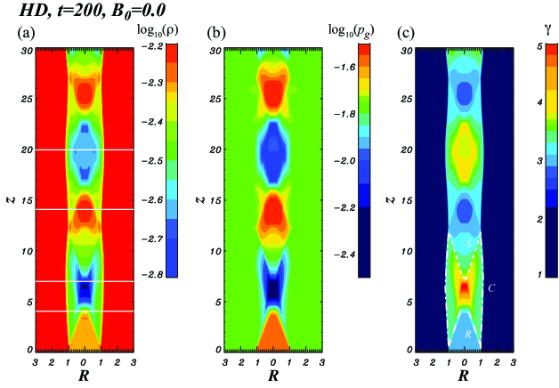
Figure 1.— Case HD. 2D plots of: (a) the rest-mass density, (b) the gas pressure, and (c) the Lorentz factor. The white solid lines in panel (a) indicate the locations along the $z$ axis used for the 1D plots in Fig. 2. Shown instead in panel (c) with dashed, dotted and dash-dotted lines are the worldlines of the rarefaction waves ($R$), of the the shock waves ($S$), and of the contact discontinuities ($C$), respectively.

In the simulations presented here, a preexisting cylindrical flow is established across the simulation domain with jet radius $R_{j}=1$. This setup represents a jet far behind the leading-edge Mach disk and bow shock (see, e.g.,  Mizuno et al., 2007, 2014). The flow is surrounded by a higher rest-mass density unmagnetized ambient medium. In all simulations the rest-mass density ratio is $\eta=\rho_{j}/\rho_{a}=5\times 10^{-3}$, where the subscripts $j$ and $a$ refer to jet and ambient values, respectively. The ambient rest-mass density is constant with $\rho_{a}=1.0\,\rho_{0}$. The jet speed is $v_{j}=0.9428$ in the $z$ direction and $\gamma_{j}=3$ with local Mach number $M_{s}=1.69$. We assume that the jet is initially uniformly over-pressured with $p_{g,j}=1.5\,p_{g,a}=1.5\,p_{g,0}$ where $p_{g,0}$ is in units of $\rho_{0}$ (see, e.g.,  Gómez et al., 1995, 1997; Agudo et al., 2001; Mimica et al., 2009). The gas pressure in the ambient medium is constant.

In order to investigate the effect of the magnetic field on the recollimation-shock structure, we have considered three different topologies: axial (or poloidal), toroidal, and helical. More specifically, for the axial-field case, the initial magnetic field $B$ is uniform and parallel to the jet flow with $B_{z}=B_{0}$, while for the toroidal-field case, we adopt the profile used by Lind et al. (1989) and Komissarov (1999) with

$$B_{\phi}=\left\{\begin{array}[]{llll}B_{0}{R/R_{m}}&\qquad\mbox{if\quad}&R&<R_{m}\,,\\ B_{0}{R_{m}/R}&\qquad\mbox{if\quad}R_{j}\geq&R&\geq R_{m}\,,\\ 0&\qquad\mbox{if\quad}&R&>R_{j}\,,\end{array}\right.$$ (12)

where the magnetization radius $R_{m}=R_{j}/4$. Finally, for the helical-field case, we chose a force-free helical magnetic field with constant magnetic “pitch”, as the one used in Mizuno et al. (2009, 2011, 2014). The poloidal and toroidal magnetic field components are given by

$$B_{z}={B_{0}\over 1+(R/a)^{2}}\,,\qquad B_{\phi}={B_{0}(R/a)\over 1+(R/a)^{2}}\,,$$ (13)

where $a$ is the characteristic radius of the magnetic field (the toroidal field component is maximum at radius $a$). The initial magnetic pitch is defined as

$$P_{0}\equiv\frac{R}{R_{j}}\left(\frac{B_{z}}{B_{\phi}}\right)=\frac{a}{R_{j}}\,,$$ (14)

which is independent of $B_{0}$ and such that a smaller $P_{0}$ refers to an increased magnetic helicity. In the magnetic helical-field case, we choose $a=R_{j}/2$, so that the initial magnetic field has constant helicity and pitch, with $P_{0}=1/2$. The values chosen for the initial $B_{0}$ and the corresponding values of the plasma beta parameter, $\beta_{p}\equiv p_{g}/p_{m}=2p_{g}/b^{2}$ (averaged and local minimum), as well as the magnetization parameter $\sigma\equiv b^{2}/\rho h$ (averaged and local maximum) are listed in Table 1 for each model. Note that in all cases the relativistic jet is kinematically dominated for all values of $B_{0}$.

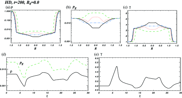
Figure 2.— Upper row: 1D profiles perpendicular to jet axis of: (a) the rest-mass density, (b) the gas pressure, and (c) the Lorentz factor as measured at $z=4$ (red dotted), $7$ (black solid), $14$ (green dashed), and $20$ (blue dash-dotted), respectively. Lower row: 1D profiles along the jet axis ($R=0$) of: (d) the rest-mass density (solid) and the gas pressure (green dashed), and (e) the Lorentz factor. All panels refer to $t_{s}=200$.

Case	$B$-field	$B_{0}$	$\langle\beta_{p}\rangle$	$\beta_{p,{\rm min}}$	$\langle\sigma\rangle$	$\sigma_{\rm max}$
HD	–	$0.0$	–	–	–	–
MHD-a	axial	$0.1$	$6.2$	$5.3$	$8.4\times 10^{-2}$	$9.0\times 10^{-2}$
MHD-b	toroidal	$0.2$	$140.5$	$13.3$	$1.1\times 10^{-2}$	$3.6\times 10^{-2}$
MHD-c	helical	$0.2$	$10.8$	$1.3$	$1.4\times 10^{-1}$	$3.6\times 10^{-1}$

Table 1Basic properties of the various cases simulated. Listed are the magnetic-field topology, the initial magnetic-field strength $B_{0}$, the average and minimum plasma beta parameters $\langle\beta_{p}\rangle$ and $\beta_{p,{\rm min}}$, as well as the average and maximum magnetization parameters $\langle\sigma\rangle$ and $\sigma_{\rm max}$.

The computational domain is $5\,R_{j}\times 30\,R_{j}$ with a uniform grid of $(R,z)=(128,300)$ computational zones. We impose outflow boundary conditions on the surfaces at $R=R_{\rm max}$ and $z=z_{\rm max}$. At $z=0$ we use fixed boundary conditions and continuously inject the over-pressured jet into the computational domain. The axisymmetry implies reflecting boundary conditions at $R=0$.

3. Results

In what follows we present the results of the simulations going through the four different magnetic-field configurations considered, i.e., cases HD, MHD-a, MHD-b, and MHD-c.

3.1. Purely hydrodynamic jet

We start our discussion of the results by illustrating what can be considered our reference configuration, that is, a purely hydrodynamical jet (case HD). Figure 1 shows 2D plots of the rest-mass density, gas pressure and Lorentz factor for the hydrodynamic case at $t_{s}=200$, where $t_{s}$ is in units of $R_{j}$. Multiple recollimation shocks and rarefactions are evident along the jet propagation direction. Downstream of the inlet the over-pressured jet produces initially a weak conical shock that propagates into the ambient medium and a quasi-stationary conical rarefaction wave that propagates into the jet (dashed lines in panel (c) of Fig. 1). The initial shock is rather weak because of the small initial pressure discontinuity and leads to relatively smooth transition between jet and ambient medium. The over-pressured jet expands (following contact discontinuities, dash-dotted lines in Fig. 1) and the rarefaction wave leads to the conversion of thermal energy into kinetic energy of the jet (see, e.g.,  Aloy & Rezzolla, 2006; Matsumoto et al., 2012). The resulting acceleration is however rather modest given the choice made here for the initial conditions.

One-dimensional (1D) profiles of hydrodynamic quantities perpendicular to the jet at axial positions $z=4$, $7$, $14$, and $20$ are shown in the upper row of Fig. 2 and help interpret the dynamics of the recollimation shocks. Note that at $z\simeq 4$ the conical rarefaction wave converges to the jet axis and at this point the rest-mass density and pressure drop significantly and the flow is considerably accelerated, going from $\gamma\sim 3$ to $\sim 4.6$ (see the solid lines in Fig. 2). At the same time, the convergence of the rarefaction wave towards the jet axis leads to strong gas-pressure gradients, which slow jet expansion. The radial expansion of the jet ceases at $z\simeq 7$ and at $z\gtrsim 7$ the jet starts to contract. Beyond $z\simeq 8$, a conical shock wave moves outward from the jet axis (see dotted lines in the panel (c) of Fig. 1) and reaches the jet edge at $z\simeq 13$. At the conical shock, between $z\simeq 8-13$, the rest-mass density and gas pressure increase and the jet Lorentz factor decreases. Furthermore, when the shock encounters the contact discontinuity at $z\simeq 13$, the jet structure has mostly returned to the initial structure, albeit at slightly higher pressure and lower velocity in the jet. The innermost recollimation structures become stationary within several light crossing times.

The panels in the bottom row of Fig. 2 offer a complementary view and, in particular, they show 1D profiles of hydrodynamical quantities along the jet axis, i.e., at $R=0$. Note that, as one would expect, the pressure profile follows exactly that of the rest-mass density as a result of the ideal-gas equation of state employed. The Lorentz factor, on the other hand, is inversely proportional to the rest-mass density, so that the energy conversion from thermal to kinetic operated by the rarefaction wave leads to a maximum in the Lorentz factor there where the rest-mass density has a minimum. Additional accelerations (i.e., peaks in the Lorentz factor) can be seen at $z\simeq 17-22$, but these are less pronounced as the second set of rarefaction waves are not as efficient in reducing the rest-mass density locally. Note also that after the first cycle of recollimation shocks and rarefaction waves, the jet does not return to the initial conditions and so the subsequent recollimation shocks and rarefactions are weaker overall.

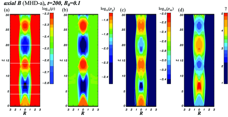
Figure 3.— Case MHD-a. 2D plots of: (a) the rest-mass density, (b) the gas pressure, (c) the magnetic pressure, and (d) the Lorentz factor for the axial magnetic-field case with $B_{0}=0.1$. The white solid lines in panel (a) indicate the locations along the $z$ axis used for the 1D plots in Fig. 4. All panels refer to $t_{s}=200$. The white solid lines in panel (a) indicate the 1D plot locations in Fig. 4.

3.2. Axial magnetic field

Next, we consider the dynamics of the recollimation shocks when an axial magnetic field is present initially (case MHD-a). Figure 3 shows 2D plots of the rest-mass density, gas pressure, Lorentz factor and magnetic pressure for the axial field case with $B_{0}=0.1$ (MHD-a) at $t_{s}=200$.

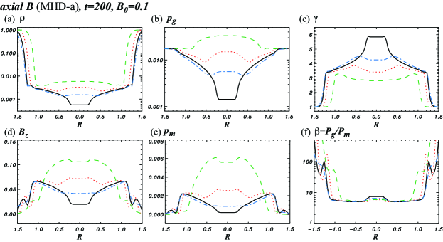
Figure 4.— 1D profiles perpendicular to jet axis of: (a) the rest-mass density, (b) the gas pressure, (c) the Lorentz factor, (d) the axial magnetic field, (e) the magnetic pressure, and (f) the plasma beta. Different lines refer to $z=4$ (black solid), $7$ (red dotted), $14$ (green dashed), and $20$ (blue dash-dotted). All quantities refer for the axial magnetic-field case (MHD-a) with $B_{0}=0.1$ and $t_{s}=200$.

As in the hydrodynamic case discussed in the previous Section, immediately downstream of the inlet, the over-pressured axially magnetized jet produces a weak conical shock that propagates into the ambient medium and a quasi-stationary conical rarefaction wave that propagates into the jet. Also in this case, the flow is boosted as a result of the exchange from thermal energy to kinetic energy. More precisely, at $z\simeq 4.5$ the conical rarefaction wave converges to the jet axis and the rest-mass density, the gas- and the magnetic pressures drop significantly, leading to an acceleration of the flow from $\gamma\sim 3$ to $\sim 6.0$ (see the solid lines in Fig. 4).

Note that the acceleration is larger than in the hydrodynamic case because the rarefaction wave is stronger and the latter is stronger because the axial magnetic field pressure acts in concert with the gas pressure but with different dependence on the jet radius. Similar results were obtained in 2D planar simulations of a flow bounded by a lower pressured ambient medium (Mizuno et al., 2008; Zenitani et al., 2010). Furthermore, downstream of the rarefaction the gas pressure decreases more than the magnetic pressure and the plasma beta decreases.

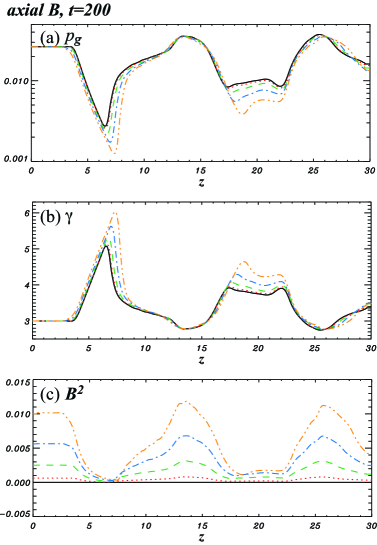
Figure 5.— 1D profiles along the jet axis ($R=0$) of: (a) the gas pressure, (b) the Lorentz factor, and (c) the magnetic pressure for the axial magnetic-field case. Different lines refer to different values of the initial magnetic-field strength, i.e., $B_{0}=0$ (black solid), $0.025$ (red dotted), $0.05$ (green dashed), $0.075$ (blue dash-dotted), and $0.1$, respectively (orange dash-double-dotted). All panels refer to $t_{s}=200$.

Figure 4 reports 1D profiles of various physical quantities perpendicular to the jet axis at axial positions $z=4$, $7$, $14$, and $20$ [see white solid lines in panel (a) of Fig. 3]. In this way it is possible to appreciate that the convergence of the rarefaction wave towards the jet axis leads to strong pressure gradients (both gas and magnetic), which slow jet expansion. Indeed, the radial expansion ceases at $z\simeq 7$ and at $z\gtrsim 7$ the jet starts to contract. Beyond $z\simeq 8$, a conical shock wave moves outward from the jet axis and reaches the jet edge at $z\simeq 13$. When the shock encounters the contact discontinuity at $z\simeq 13$, the jet has mostly returned to the initial structure, albeit at a slightly lower velocity.

In summary, while maintaining many similarities with the purely hydrodynamical evolution, the presence of an axial magnetic field leads to stronger recollimation shock and rarefaction waves. In turn, because the AR booster is sensitive only to jumps in the specific enthalpy and not on whether a magnetic field is present, the sharper discontinuities in the flow lead to stronger boosts (see also the discussion in Sect. 4).

Finally, to assess the role played by the initial strength of the magnetic field $B_{0}$ on the subsequent dynamics, we show in Fig. 5 the 1D profiles of the gas pressure, of the Lorentz factor and of the magnetic-field strength along the jet axis, i.e., at $R=0$. The different lines refer respectively to $B_{0}=0.0$, i.e., the purely hydrodynamical evolution, as well as $B_{0}=0.025$, $0.05$, $0.075$, and $0.1$ respectively. The main feature to note in this case is that an increasingly stronger axial magnetic field does not introduce qualitative changes in the flow dynamics. Indeed, the changes are only quantitative, with smaller values for the rest-mass density and pressure and consequently larger values of the Lorentz factor. It follows that the observational knowledge of the plasma velocity at different positions in the jet could be used to deduce the strength of the magnetic field in the jet.

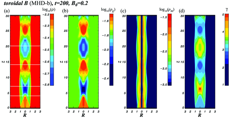
Figure 6.— Case MHD-b. The same as in Fig. 3 but for the toroidal magnetic-field case with $B_{0}=0.2$.

3.3. Toroidal magnetic field

We continue our investigation by considering the dynamics of the recollimation shocks when a toroidal magnetic field is initially present (case MHD-b). In particular, Fig. 6 shows 2D plots of the rest-mass density, gas pressure, magnetic pressure and Lorentz factor for the toroidal field case with $B_{0}=0.2$ at $t_{s}=200$.

The general behavior is similar to both the hydrodynamic and axial magnetic-field cases. Namely, the over-pressured toroidally magnetized jet produces an initially weak conical shock that propagates into the ambient medium and, at the same time, a conical rarefaction wave that propagates into the jet. The latter expands radially, but the rarefaction waves produced are also responsible for the conversion of the thermal energy of the plasma into kinetic energy of the jet following the basic mechanism of the AR booster. At $z\simeq 4.5$, this process leads to an increase in the Lorentz factor of flow that is accelerated from $\gamma\sim 3$ to $\sim 4.2$ (see the solid lines in Fig. 7c).

Despite these analogies, the toroidal-field case also presents an important qualitative difference. Although it increases, the maximum value attained by the jet Lorentz factor is smaller than in the hydrodynamical case; this is in contrast with what was found for the axial magnetic-field case in the previous Section. The origin of this different behaviour is to be found in the magnetic tension introduced by the toroidal magnetic field and that essentially resists both inwards and outwards motions. This is quite visible in the behaviour along the $z$ direction of the magnetic pressure [see panel (c) of Fig. 6], which shows a “pinching” effect at $z\sim 4,13$ and $z\sim 25$, which also correspond to the locations where the rarefaction waves converge at the jet axis [see panel (a) of Fig. 6].

This structure in the magnetic pressure also appears in the radial profile of the plasma beta in Fig. 7, which reports 1D profiles of several quantities perpendicular to the jet at axial positions $z=4$, $7$, $14$, and $20$. In particular, the panel (f) shows that plasma beta has two minima of the order of $\beta_{p}\sim 20$ on either side of the jet axis where the toroidal magnetic field is at a maximum (i.e., at $R\sim\pm 0.3$); this behaviour should be contrasted with the corresponding one shown in (f) of Fig. 4 for the axial magnetic-field case, where instead the smallest value of the beta parameter is $\beta_{p}\sim 5$.

Figure 7.— The same as in Fig. 5, but for the toroidal-magnetic field case.

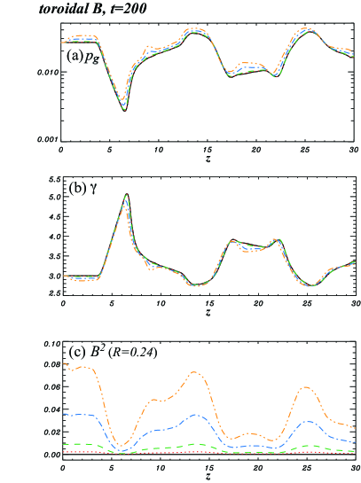
Figure 8.— The same as in Fig. 5, but for the toroidal magnetic field case with $B_{0}=0$ (black solid), $0.05$ (red dotted), $0.1$ (green dashed), $0.2$ (blue dash-dotted), and $0.3$ (orange dash-double-dotted).

The presence of a toroidal magnetic field also alters considerably the flow after the shock encounters the contact discontinuity at $z\simeq 13$, breaking the appearance of a periodicity in the recollimation-shock structure. Interestingly, both the gas pressure and the Lorentz factor show an “O”-shaped structure around $z\simeq 16-23$ [see panels (b) and (d) of Fig. 6], with both of these quantities reaching a local minimum around $z\simeq 20$ and $R\simeq 0$ [see also panels (b) and (f) of Fig. 7].

In summary, the presence of a toroidal magnetic field leads to weaker recollimation shocks and rarefaction waves, with a more complicated downstream structures than those found for the hydrodynamic and axial magnetic field cases. If observed, this different phenomenology should provide useful information to deduce the properties of the magnetic-field topology in the jet and, in particular, to establish whether this is purely toroidal.

Finally, also in this case, we report in Fig. 8 the 1D profiles of the gas pressure and of the Lorentz factor along the jet axis, i.e., at $R=0$, as well as the magnetic-field strength along a direction slightly off the axis, i.e., at $R=0.24$ (we recall that the magnetic field is zero along the axis). The figure aims at establishing the variations introduced by the initial magnetic-field strength $B_{0}$ and so different lines refer to $B_{0}=0.0$ (i.e., the purely hydrodynamical case) as well as to $B_{0}=0.05$, $0.1$, $0.2$, and $0.3$. Perhaps not remarkably, only minimal changes are visible in the radial profiles of the rest-mass density, of the gas pressure and of the jet Lorentz factor as the magnetic field strength is increased. This is mostly due to the fact that the magnetic tension introduced by the toroidal magnetic field acts mostly in the $R$ direction, producing only high-order variations in the direction of propagation of the jet. Such a behaviour is markedly different from the one encountered in the case of an axial magnetic field, and indeed Fig. 8 should be contrasted with the corresponding Fig. 5.

3.4. Helical magnetic field

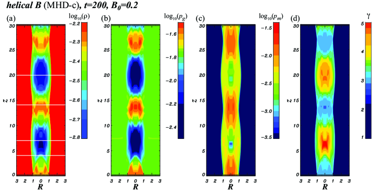
Figure 9.— Case MHD-c. The same as in Fig. 3, but for the helical magnetic-field case with $B_{0}=0.2$.

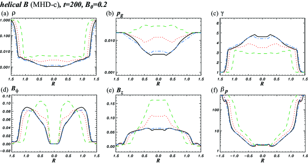
Figure 10.— 1D profiles perpendicular to the jet axis of: (a) the rest-mass density, (b) the gas pressure, (c) the Lorentz factor, (d) the toroidal magnetic field, (e) the axial magnetic field, and (f) the plasma beta as measure at $z=4$ (black solid), $7$ (red dotted), $14$ (green dashed), and $20$ (blue dash-dotted). All panels refer to the helical magnetic-field case with $B_{0}=0.2$ at $t_{s}=200$.

Finally, we consider the dynamics of the recollimation shocks when a helical magnetic field is present initially (case MHD-c), with constant initial pitch $P_{0}=1/2$. As for the other cases, we show in Fig. 9 2D plots at $t_{s}=200$ of the rest-mass density, of the gas- and magnetic pressures, and of the Lorentz factor when $B_{0}=0.2$.

Similar to the other magnetic-field topologies, also in this case the over-pressured jet produces an initially weak conical shock that propagates into the ambient medium and a conical rarefaction wave that propagates into the jet. Again, conservation across the rarefaction wave of $\gamma h$ implies that a conversion of thermal energy to jet kinetic energy takes place across the rarefaction wave, with a consequent acceleration of the flow. Although the pitch considered here is less than one, so that the toroidal magnetic field is larger than the axial one at least initially, the effective behaviour of the plasma is closer to the one seen in the case of an axial magnetic field than in the case of a toroidal magnetic field. In particular, the increase in the Lorentz factor is larger than in the hydrodynamical case, although only slightly, i.e., with downstream Lorentz factors going up to $\gamma\simeq 5.0$. On the other hand, as we have encountered in the previous section for a purely toroidal magnetic field, the small pitch also implies that the plasma beta reach its minimum values there [cf., (f) in Fig. 7].

Figure 10 reports the 1D profiles of several quantities perpendicular to the jet axis at the positions $z=4$, $7$, $14$, and $20$. Note the close analogies with the corresponding behaviours shown in Fig. 7 in the case of a purely toroidal magnetic field. Also here, the convergence of the rarefaction waves towards the jet axis leads to strong gas and magnetic-pressure gradients, which ultimately slow the jet expansion. This ceases at $z\simeq 10-14$, when weak shocks return the jet to an over-pressured structure and with a reduced Lorentz factor and rather different conditions than the initial ones.

In summary, the presence of a helical magnetic field in the jet leads to a rather complex behaviour in both the recollimation shock and rarefaction structure. While the flow can be magnetically dominated with plasma beta of order unity, the Lorentz factor is increased with respect to the purely hydrodynamical case, mimicking the behaviour seen for purely axial fields. This global behaviour is clearly influenced in part by our choice for the initial pitch and we expect that if a lower magnetic pitch parameter is chosen, corresponding to a more tightly wrapped helical field, the toroidal field will dominate over the axial field effects, with a sub-hydrodynamical Lorentz factor boost (see also the discussion in Section 4).

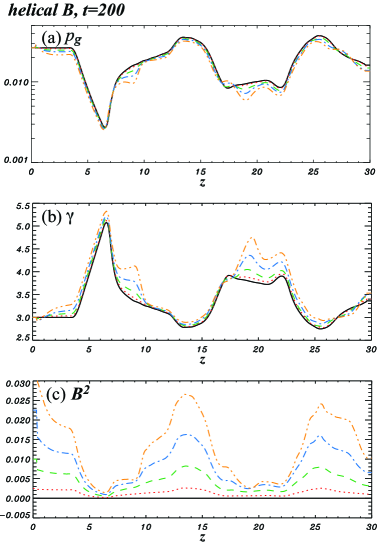
Figure 11.— The same as in Fig. 5, but for the helical magnetic-field case with $B_{0}=0$ (black solid), $0.05$ (red dotted), $0.1$ (green dashed), $0.15$ (blue dash-dotted), and $0.2$ (orange dash-double-dotted).

Finally, the role played by the initial strength of the magnetic field $B_{0}$ on the subsequent dynamics is shown in Fig. 11, which reports the 1D profiles along the jet’s axis of the gas pressure, of the Lorentz factor and of the magnetic field strength. Again, the different lines refer respectively to $B_{0}=0.0$, and to $B_{0}=0.05$, $0.1$, $0.15$, and $0.2$ (dotted, dashed, dash-dotted and dash-double-dotted lines, respectively). Also in this case, it is possible to observe how the phenomenology of the helical field is a combination of the one seen for purely axial and purely toroidal magnetic fields. In particular, as in the toroidal-field case, the gas pressure shows only modest changes along the $z$ direction when the magnetic field is increased. On the other hand, as in the axial-field case, the Lorentz factor shows peaks that increase and move downstream with increasing magnetic-field strengths.

4. Jet Acceleration

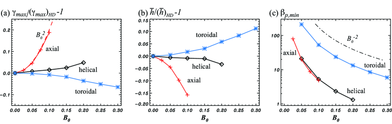
Figure 12.— Dependence of: (a) the relative difference of the maximum Lorentz factor $\gamma_{\rm max}/(\gamma_{\rm max})_{{}_{\rm HD}}-1$, (b) the relative difference of the specific enthalpy $\bar{h}/(\bar{h})_{{}_{\rm HD}}-1$, and (c) the minimum plasma beta. All quantities are shown as a function of the initial magnetic-field strength, $B_{0}$ in the case of axial (red crosses), toroidal (blue stars), and helical magnetic fields (black diamonds) with $P_{0}=0.5$. The red dashed line in panel (a) indicates a quadratic fit [cf., Eq. (15)], while the black dot-dashed line in panel (c) refers to a $B_{0}^{-2}$ scaling.

In the previous Sections we have illustrated in detail how a robust feature of the recollimation shocks considered here is the acceleration of the flow downstream of the inlet as a result of the AR booster. We have also remarked that the occurrence of this acceleration is the result of the conversion of the plasma thermal energy into kinetic energy of the jet, or, more precisely, of the conservation of the quantity $\gamma h$ across a rarefaction wave (Aloy & Rezzolla, 2006). In addition, we have discussed how different magnetic field topologies lead to systematically different values of the maximum increase in the Lorentz factor measured downstream of the inlet, i.e., $\Delta\gamma_{\rm max}\equiv{\rm max}({\gamma})-\gamma_{0}$. What we have not yet discussed, however is how this accelerating mechanism depends on our choice of the initial magnetic-field strength, $B_{0}$.

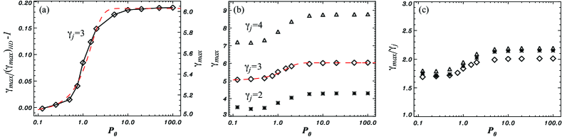
Figure 13.— Left panel: Dependence of the maximum Lorentz factor $\gamma_{\rm max}$ (right vertical axis) and relative difference of the maximum Lorentz factor relative to the purely hydrodynamical case $\gamma_{\rm max}/(\gamma_{\rm max})_{{}_{\rm HD}}-1$ (left vertical axis) as a function of the initial magnetic pitch, $P_{0}$; the initial jet Lorenz factor is set to $\gamma_{j}=3$; the red dashed line indicates the fitting with a hyperbolic tangent function [cf., Eq. (16)]. Central panel: Dependence of the maximum Lorentz factor as a function of the initial magnetic pitch, for three different values of the initial jet Lorenz factor $\gamma_{j}=2$ (stars), $3$ (diamonds), and $4$ (triangles); the red dashed line indicates the fitting as in the left panel. Right panel:. The same as in the central panel but when the maximum Lorentz factors are normalized to the initial one; note that in this case all curves essentially overlap. All cases refer to an initial magnetic field $B_{0}=0.1$.

This point is addressed in the left panel of Fig. 12, which reports the relative increase of the Lorentz factor with respect to the purely hydrodynamical evolution, namely, $\Delta\gamma_{\rm max}/(\gamma_{\rm max})_{{}_{\rm HD}}\equiv\gamma_{\rm max}/(\gamma_{\rm max})_{{}_{\rm HD}}-1$, as a function of the initial magnetic field. Obviously, this quantity can either be positive or negative and provides a direct measure of the fractional boost. Shown with different symbols are the different magnetic-field topologies, with crosses referring to the axial magnetic field (case MHD-a), diamonds to the helical magnetic-field (case MHD-c), and star crosses to the toroidal magnetic-field (case MHD-b).

When presented in this manner, it is then straightforward to realize that axial and helical initial magnetic fields lead to Lorentz boosts that are larger than in the hydrodynamical case, while the opposite is true for purely toroidal magnetic fields, for which an acceleration is still present but this is smaller than in the hydrodynamical case. We have already discussed in the previous Sections that the origin of this different behaviour has to be found in the fact that an axial magnetic field adds an effective gas pressure and results in larger rest-mass density and pressure gradients across the rarefaction waves induced downstream of the inlet. In turn, the AR booster translates these stronger waves into larger accelerations of the flow. It is also instructive that, in the case of a purely axial magnetic field, the behaviour of the relative boost has a simple quadratic dependence on the initial magnetic field. This is simply because the relative boost scales as

$$\frac{\Delta\gamma_{\rm max}}{(\gamma_{\rm max})_{{}_{\rm HD}}}\propto\frac{p}{p_{g}}-1=\frac{p_{m}}{p_{g}}\propto B_{z}^{2}\,.$$ (15)

This is confirmed by the very good match between the numerical data and a quadratic fit, which is indicated with a red dashed line.

Also shown in Fig. 12, but in the middle panel, are the fractional differences in the specific enthalpy at the position of the maximum Lorentz factor, i.e., $\bar{h}/(\bar{h})_{{}_{\rm HD}}-1$. Here too, different symbols refer to the various magnetic-field topologies (cf., left panel) and different initial strengths. Clearly, this panel offers a complementary view to the one in the left panel and summarizes much of what already discussed in the previous Sections. Namely, that axial and helical magnetic fields leads to smaller values of the specific enthalpy in the downstream solution, in contrast to the case of toroidal magnetic fields where instead the values of the specific enthalpy at Lorentz-factor maximum increases with the initial magnetic field. Finally, shown in the right panel of Fig. 12 is the behaviour of the minimum plasma beta $\beta_{p,{\rm min}}$ as a function of the initial magnetic field. Interestingly, all magnetic-field topologies show the same (and expected) quadratic dependence as $B^{-2}_{0}$.

4.1. Dependence on magnetic pitch

As discussed in Section 2, in the case of a helical magnetic field, we have an additional degree of freedom represented by the initial magnetic pitch as defined in Eq. (14). By suitably choosing the initial pitch, i.e., the ratio $a/R_{j}$, it is possible to scan the range of possible magnetic-field configurations, which range from an essentially toroidal magnetic field for $P_{0}\ll 1$ to an axial axial magnetic field for $P_{0}\gg 1$.

Given this freedom in the parameterization, and given that different magnetic-field topologies lead to different amplifications to the AR booster, it is interesting to ask whether a correlation exists between the initial pitch and the increase in the maximum Lorentz factor downstream of the inlet. This is shown in Fig. 13, which shows $\Delta\gamma_{\rm max}/(\gamma_{\rm max})_{{}_{\rm HD}}$ as a function of the initial pitch $P_{0}$ for a number of simulations carried out with $B_{0}=0.1$. Interestingly, we found that the relative increase in the maximum Lorentz factor has a very clear dependence with the pitch, smoothly joining the two extreme cases of a toroidal and axial magnetic fields, respectively. Furthermore, the transition between the two regimes takes place at $P_{0}\gtrsim 1$, that is, when $a\gtrsim R_{j}$, saturating to the axial field case when $a\simeq 10\,R_{j}$. Finally, the dependence can be accurately approximated with a simple expression of the type

$$\gamma_{\rm max}\simeq c_{1}+c_{2}\tanh[c_{3}(P_{0}-1.0)]\,,$$ (16)

where $c_{1}\simeq 5.43,c_{2}\simeq 0.6$, and $c_{3}\simeq 0.8$, and is indicated with the red dashed line in Fig. 13.

The relevance of expression (16) is that it provides, at least in principle, yet another useful tool to deduce the properties of the magnetic-field topology from the observations of the jet dynamics. Indeed, if radio-astronomical observations could provide a reliable measure of the Lorentz factor in the bulk of the jet and at its base, i.e., $\gamma_{\rm max}$ and $\gamma_{j}$, then expression (16) would provide a simple way to deduce the degree of helicity of the magnetic field in the jet. This is because while the relation between $\gamma_{\rm max}$ and the pitch $P_{0}$ changes with the initial Lorentz factor in the jet $\gamma_{j}$, the fact that $\gamma_{\rm max}$ and $\gamma_{j}$ scale linearly [cf., left panel of Fig. 15] implies that the functional dependence of $\gamma_{\rm max}/\gamma_{j}$ with $P_{0}$ will not change. This is shown in the right panel of Fig. 13. Hence, once and if $\gamma_{\rm max}/\gamma_{j}$ is measured, a direct estimate on $P_{0}$ is possible, which is only weakly dependent on the jet overpressure. Conversely, if the magnetic field pitch angle could be determined, e.g., from polarimetric observations, then it could be possible to estimate $\gamma_{\rm max}$. Such a measurement would obviously be of great importance for the interpretation of the very rapid TeV variability in AGN jets.

5. Conclusion

We have performed 2D SRMHD simulations of the propagation of an over-pressured relativistic jet leading to the generation of a series of recollimation shocks and rarefaction waves. The overall dynamics of this process is rather well known. Downstream of the inlet, the jet produces a weak conical shock that propagates into the ambient medium and a quasi-stationary conical rarefaction wave that propagates inwards. The significant drops in rest-mass density and pressure produced by the rarefaction waves are also responsible for the conversion of the thermal energy into kinetic energy of the jet (see, e.g.,  Aloy & Rezzolla, 2006; Matsumoto et al., 2012). This is a purely relativistic effect that develops in the presence of strong tangential discontinuities in the flow (Rezzolla & Zanotti, 2002), and that leads to a consistent and robust boost of the fluid. In addition, the nonlinear interaction of the shocks and rarefaction waves lead to a stationary and multiple recollimation-shock structure along the jet, which has been reproduced by a number of the hydrodynamic simulations under different physical conditions (see, e.g.,  Gómez et al., 1997; Komissarov & Falle, 1997; Agudo et al., 2001; Aloy et al., 2003; Roca-Sogorb et al., 2008, 2009; Mimica et al., 2009; Matsumoto et al., 2012).

We have here extended previous hydrodynamic work to determine the effect that magnetic fields with axial, toroidal, and helical topologies have on the jet dynamics. In particular, we have found that an axial magnetic field behaves as an additional gas pressure, leading to a sharper recollimation-shock structure and thus larger flow accelerations. On the other hand, a toroidal magnetic field tends to reduce the inward motion of the rarefaction waves, thus leading to a weaker recollimation-shock structure and accelerations that are even smaller than in the case of a purely hydrodynamical evolution. Finally, a helical magnetic field tends to yield a behaviour which is a combination of those observed for purely axial/toroidal magnetic fields, with larger Lorentz factors, but also with a rather complex recollimation-shock substructure.

As predicted by the basic properties of the AR booster, we have found that the boost in the jet flow, as measured in terms of the maximum Lorentz factor, is anti-correlated with the values of the specific enthalpy. Furthermore, the boost grows quadratically with the initial magnetic field in the case of a purely axial flow, at smaller rates in the case of a helical magnetic field, and it decreases systematically when a purely toroidal magnetic field is present. Finally, we have shown that the maximum Lorentz factor exhibits a smooth behaviour in terms of the initial pitch in the case of an axial magnetic field.

Stationary components are commonly seen in parsec-scale VLBI observations of AGN jets (see, e.g.,  Jorstad et al., 2005; Lister et al., 2013; Cohen et al., 2014), being normally associated with recollimation shocks. Studying in detail the structure in these stationary components for a direct comparison with our simulations requires however resolving the jet structure across the jet width. This can be achieved through “regular” cm-VLBI observations of nearby sources, like M87, but for the majority of the AGN jets it would require a significant increase in angular resolution. This can be obtained through VLBI observations at even shorter wavelengths, in which the 3 mm GMVA (Global Millimeter VLBI Array) and 1.3 mm VLBI observations with the Event Horizon Telescope and Black-Hole Cam projects can achieve angular resolutions between 50 and 20 microarcseconds (see, e.g.,  Fish et al., 2014; Krichbaum et al., 2013), and through space VLBI observations. The space VLBI mission “RadioAstron” has recently successfully achieved ground-space fringe detections for observations at 1.3 cm on baselines longer than eight Earth diameters, allowing imaging the innermost regions in AGN jets with an unprecedented angular resolution of $\sim$ 20 microarcseconds (Gómez et al., 2015).

Whilst the range of simulations carried out here have tried to explore a rather large portion of the space of parameters, a number of improvements on the approach followed here can be made. First, even though we have assumed an over-pressured jet to produce the recollimation-shock structure, a pressure mismatch between jet and ambient medium arises naturally if the pressure in the ambient medium decreases with distance from the central object. In this case, the recollimation-shock structure depends on the ambient-medium pressure scale (see, e.g.,  Gómez et al., 1997; Komissarov & Falle, 1997; Agudo et al., 2001; Aloy et al., 2003; Mimica et al., 2009; Kohler et al., 2012; Matsumoto et al., 2012; Porth & Komissarov, 2014). Although we do not expect that significant qualitative differences will emerge from a more realistic modelling of the ambient medium, we will extend the current investigation to include larger overpressure ratios, as well as declining pressure profiles outside the jet.

Second, in this work we assume the relativistic jet is kinematically dominated initially for all values of the initial magnetic field. However, magnetically dominated relativistic jets (Poynting-flux dominated jets) might be plausible from the results of previous analytical (e.g.,  Heyvaerts & Norman, 2003; Beskin & Nokhrina, 2009; Lyubarsky, 2009) and numerical studies (e.g.,  Komissarov et al., 2006; Tchekhovskoy et al., 2009; Porth et al., 2011; McKinney et al., 2012). We will investigate this type of relativistic jets in future work.

Third, it is clear that the magnetic modifications of the recollimation-shock structure found here may affect in a significant way the signatures of stationary components seen in several AGN jets, especially in polarized flux. An even clearer signature difference may be obtained when a shock like disturbance propagates through the stationary recollimation-shock structure. In view of this, we will investigate the propagation of such a shock-like disturbance through a magnetized recollimation shock and calculate the corresponding emission following the approach presented in, e.g., Gómez et al. (1997).

Finally, although our simulations show that the recollimation-shock strength depends on the jet magnetization and magnetic field structure, it is clear that its observed appearance as imaged by VLBI would also depend on the jet-viewing angle, and is obviously influenced by Doppler-boosting effects. Hence, depending on the jet bulk flow Lorentz factor and viewing angle, the Doppler boosting may cancel, or even reverse, the increased emissivity obtained in the recollimation shock and due to the enhanced particle and magnetic-field energy rest-mass density (see, e.g.,  Gómez et al., 1997; Aloy et al., 2003; Roca-Sogorb et al., 2008, 2009; Mimica et al., 2009). These effects will also be the focus of future investigations.

Appendix A Convergence Tests

A.1. Large-scale hydrodynamical jet

Due to the uniform ambient medium, the modifications of the recollimation-shock and rarefaction-wave structures is expected to be rather small and a quasi-periodic structure should develop on larger axial scales (see also Matsumoto et al., 2012). In this Appendix we test this assumption, and hence the development of a self-similarity in the recollimation-shock structure, by considering a purely hydrodynamical simulation having the same resolution discussed in Section 3.1, but with an extent in the $z$ direction from $0$ to $90$, that is, three times larger than what presented in the main text. The results of this simulation are reported in Fig. 14, with the top three panels referring to a two-dimensional view, and the bottom two panels to a cut along the $z$ axis at $t_{s}=600$. It is clear that the shock/rarefaction structure is periodic and with periodicity $\simeq 12R_{j}$. This separation distance depends on the initial jet velocity, over-pressure ratio between jet and ambient pressure, and opening angle of the jet.

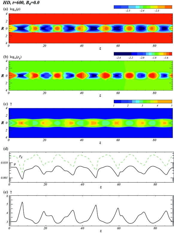
Figure 14.— Upper panels: 2D plots of: (a) the rest-mass density, (b) the gas pressure, and (c) the Lorentz factor. Lower panels: 1D profiles along the jet axis ($R=0$) of: (d) the rest-mass density (solid) and the gas pressure (green dashed), and (e) the Lorentz factor. All panels refer to $t_{s}=600$ for a purely hydrodynamical jet and an extent in the $z$ direction that is three times larger than the one considered in the main text.

A.2. Dependence on initial jet Lorentz factor and over-pressure ratio of the maximum jet Lorentz factor

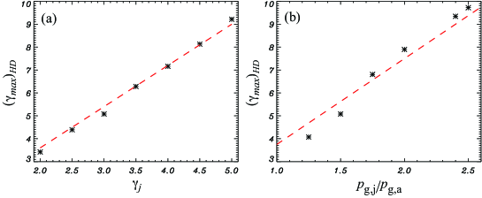
Figure 15.— Dependence of the maximum Lorentz factor in a purely hydrodynamical jet $(\gamma_{jet})_{{}_{\rm HD}}$ as a function of: (a) the initial jet Lorentz factor $\gamma_{j}$ with fixed over-pressure ratio $p_{g,j}/p_{g,a}=1.5$ and (b) the over-pressure ratio $p_{g,j}/p_{g,a}$ with fixed initial jet Lorentz factor $\gamma_{j}=3$. The red dashed lines indicate the linear fitting.

As discussed in Section 4, the relative difference of the maximum jet Lorentz factor with respect to the purely hydrodynamic case depends on the initial magnetic field strength and magnetic pitch. It is important to know the maximum jet Lorentz factor of a pure hydrodynamic case. In this Appendix, we have investigated the dependence of the maximum jet Lorentz factor of a pure hydrodynamic jet on the initial jet Lorentz factor and over-pressure ratio. Figure 15 shows $(\gamma_{max})_{{}_{\rm HD}}$ as a function of the initial jet Lorentz factor ($\gamma_{j}$) and of the over-pressure ratio ($p_{g,j}/p_{g,a}$). Clearly, $(\gamma_{jet})_{{}_{\rm HD}}$ has a simple linear dependence on both the initial jet Lorentz factor and the over-pressure ratio with a coefficient of $\simeq 1.8$ and $\simeq 3.75$ respectively, which we indicate with the red dashed lines in Fig. 15.

References

- Agudo et al. (2001) Agudo, I., Gómez, J. L., Martí, J.-M. et al. 2001, ApJ, 549, L183
- Alberdi et al. (2000) Alberdi, A., Gómez. J. L., Marcaide, J. M., Marscher, A. P., & Pérez-Torres, M. A. 2000, A&A, 361, 529
- Aloy & Rezzolla (2006) Aloy, M. A., & Rezzolla, L. 2006, ApJ, 640, L115
- Aloy et al. (2003) Aloy, M. A., Martí, J.-M., Gómez, J. L., Agudo, I., Müller, E., & Ibáñez, J.-M. 2003, ApJ, 585, L109
- Asada & Nakamura (2012) Asada, K., & Nakamura, M. 2012, ApJ, 745, L28
- Asada et al. (2014) Asada, K., Nakamura, M., Doi, A., Nagai, H., & Inoue, M. 2014, ApJ, 781, L2
- Beskin & Nokhrina (2009) Beskin, V. S., & Nokhrina, E. E. 2009, MNRAS, 397, 1486
- Casadio et al. (2013) Casadio, C., Gómez, J. L., Giroletti, M., et al. 2013, in EPJ Web of Conferences, Vol. 61, The Innermost Regions of Relativistic Jets and Their Magnetic Fields (Les Ulis, France: EDP Sciences), 06004
- Cheung et al. (2007) Cheung, C. C., Harris, D. E., & Stawarz, Ł, 2007, ApJ, 663, L65
- Cohen et al. (2014) Cohen, M. H., Meier, D. L., Arshakian, T. G., et al. 2014, ApJ, 787, 151
- Daly & Marscher (1988) Daly, R. A., & Marscher, A. P. 1988, ApJ, 334, 539
- Fish et al. (2014) Fish, V. L., Johnson, M. D., Lu R.-S., et al. 2014, ApJ, 795, 134
- Fromm et al. (2013) Fromm, C. M., Ros, E., Perucho, M., et al. 2013, A&A, 551, A32
- Gabuzda et al. (2014) Gabuzda, D. C., Cantwell, T. M., & Cawthorne, T. V. 2014, MNRAS, 438, L1
- Giroletti et al. (2012) Giroletti, M. Hada, K., Giovannini, G. et al. 2012, A&A, 538, L10
- Gómez et al. (1993) Gómez, J. L., Alberdi, A., & Marcaide, J. M. 1993, A&A, 274, 55
- Gómez et al. (1995) Gómez, J. L., Marti, J. M. A., Marscher, A. P., Ibanez, J. M. A., & Marcaide, J. M. 1995, ApJ, 449, L19
- Gómez et al. (1997) Gómez, J. L., Martí, J. M., Marscher, A. P., Ibáñez, J. M., & Alberdi, A. 1997, ApJ, 482, L33
- Gómez et al. (2015) Gómez et al. 2015, in preparation
- Harten et al. (1983) Harten, A., Lax, P. D., & van Leer, B. 1983, SIAM Rev., 25, 35
- Heyvaerts & Norman (2003) Heyvaerts, J., & Norman, C., 2003, ApJ, 596, 1240
- Jorstad et al. (2005) Jorstad, S. G., Marscher, A. P., Lister, M. L., et al. 2005, AJ, 130, 2473
- Jorstad et al. (2013) Jorstad, S. G., Marscher, A. P., Smith P. S., et al. 2013, ApJ, 773, 147
- Krichbaum et al. (2013) Krichbaum, T. P., Roy, A., Wagner, J. et al. 2013, arXiv:1305.2811
- Kohler & Begelman (2012) Kohler, S., & Begelman, M. C. 2012, MNRAS, 426, 595
- Kohler et al. (2012) Kohler, S., Begelman, M. C., & Beckwith, K. 2012, MNRAS, 422, 2282
- Komissarov (1999) Komissarov, S. S. 1999, MNRAS, 308, 1069
- Komissarov & Falle (1997) Komissarov, S. S., & Falle, S. A. E. G. 1997, MNRAS, 228, 833
- Komissarov et al. (2010) Komissarov, S. S., Vlahakis, N., & Königl, A. 2010, MNRAS, 407, 17
- Komissarov et al. (2006) Komissarov, S. S., Barkov, M., Vlahakis, N., & Königl, A. 2006, MNRAS, 380, 51
- Kovalev et al. (2008) Kovalev, Y. Y., Lobanov, A. P., Pushlarev, A. B., & Zensus, J. A. 2008, A&A, 483, 759
- Lind et al. (1989) Lind, K. R., Payne, D. G., Meier, D. L. & Blandford, R. D. 1989, ApJ, 344, 89
- Lister et al. (2013) Lister, M. L., Aller, M. F., Aller, H. D., et al. 2013, AJ, 146, 120
- Lyubarsky (2009) Lyubarsky, Y. 2009, ApJ, 698, 1570
- Marscher et al. (2008) Marscher, A. P., Jorstad, S. G., D’Arcangelo, F. D. et al. 2008, Nature, 452, 966
- Marscher et al. (2010) Marscher, A. P., Jorstad, S. G., Larionov, V. M. et al. 2010, ApJ, 710, L126
- Marscher (2014) Marscher, A. P. 2014, ApJ, 780, 87
- Matsumoto et al. (2012) Matsumoto, J., Masada, Y., & Shibata, K. 2012, ApJ, 751, 140
- McKinney et al. (2012) McKinney, J. C., Tchekhovskoy, A., & Blandford, R. D. 2012, MNRAS, 423, 2083
- Mimica et al. (2009) Mimica, P., Aloy, M.-A., Agudo, I., Martí, J. M., Gómez, J. L., & Miralles, J. A. 2009, ApJ, 696, 1142
- Mizuno et al. (2007) Mizuno, Y., Hardee, P., & Nishikawa, K.-I. 2007, ApJ, 662, 835
- Mizuno et al. (2011) Mizuno, Y., Hardee, P. E., & Nishikawa, K.-I. 2011, ApJ, 734, 19
- Mizuno et al. (2014) Mizuno, Y., Hardee, P. E., & Nishikawa, K.-I. 2014, ApJ, 784, 167
- Mizuno et al. (2009) Mizuno, Y., Lyubarsky, Y., Nishikawa, K.-I., & Hardee, P. E. 2009, ApJ, 700, 684
- Mizuno et al. (2006) Mizuno, Y., Nishikawa, K.-I., Koide, S., Hardee, P., & Fishman, G. J. 2006, arXiv:astro-ph/0609004
- Mizuno et al. (2008) Mizuno, Y., Hardee, P., Hartmann, D. H., Nishiakwa, K.-I., & Zhang, B. 2008, ApJ, 672, 72
- O’Sullivan & Gabuzda (2008) O’Sullivan, S. P., & Gabuzda, D. C. 2008, MNRAS, 400, 26
- Porth & Komissarov (2014) Porth, O., & Komissarov, S. S. 2014, arXiv:1408.3318
- Porth et al. (2011) Porth, O., Fendt, C., Meliani, Z., & Vaidya, B. 2011, ApJ, 737, 42
- Rezzolla & Zanotti (2002) Rezzolla, L. and Zanotti, O. 2002, Phys. Rev. Lett. 89, 114501.
- Rezzolla & Zanotti (2013) Rezzolla, L., & Zanotti, O. 2013, Relativistic Hydrodynamics (Oxford: Oxford University Press)
- Roca-Sogorb et al. (2010) Roca-Sogorb, M., Gómez, J. L., Agudo, I., Marscher, A. P., & Jorstad, S. G. 2010, ApJ, 712, L160
- Roca-Sogorb et al. (2008) Roca-Sogorb, M., Perucho, M., Gómez, J. L., Martí, J. M., Antón, L., Aloy, M. A., & Agudo, I. 2008, Mem. S. A. It., 79, 1174
- Roca-Sogorb et al. (2009) Roca-Sogorb, M., Perucho, M., Gómez, J. L., Martí, J. M., Antón, L., Aloy, M. A., & Agudo, I. 2009, in ASP Conf. Ser. 402, Approaching Micro-Arcsecond Resolution with VSOP-2: Astrophysics and Technologies, ed. Y. Hagiwara, E. Fomalont, M. Tsuboi, & Y. Murata (San Francisco, CA: ASP), 353
- Sapountzis & Vlahakis (2013) Sapuntzis, K., & Vlahakis, N. 2013, MNRAS, 434, 1779
- Shu & Osher (1988) Shu, C. W., & Osher, S. J. 1988, JCoPh, 77, 439
- Suresh & Huynh (1997) Suresh, A., & Huynh, H. T. 1997, JCoPh, 136, 83
- Sokolovsky et al. (2011) Sokolovsky, K. V., Kovalev, Y. Y., Pushkarev, A. B., & Lobanov, A. P. 2011, A&A, 532, A38
- Tóth (2000) Tóth, G. 2000, JCoPh, 161, 605
- Tchekhovskoy et al. (2009) Tchekhovskoy, A., McKinney, J. C., & Narayan, R. 2009, ApJ, 699, 1789
- Zenitani et al. (2010) Zenitani, S., Hesse, M., & Klimas, A. 2010, ApJ, 712, 951