Shear viscosity of the $\Phi^{4}$ theory from classical simulation

Abstract

Shear viscosity of the classical $\Phi^{4}$ theory is measured using classical microcanonical simulation. To calculate the Kubo formula, we measure the energy-momentum tensor correlation function, and apply the Green-Kubo relation. Being a classical theory, the results depend on the cutoff which should be chosen in the range of the temperature. Comparison with experimentally accessible systems is also performed.

1 Introduction

Transport coefficients, in particular shear viscosity, are very hardly accessible quantities in perturbative quantum field theory calculations. Transport is characteristic to systems where information is spread by diffusion, the time evolution is $\sim\sqrt{Dt}$, the diffusion constant being the corresponding transport coefficient. The diffusion constant itself is proportional to the quasiparticle lifetime $D\sim\tau$. This is infinite in a free gas, and inversely proportional to some powers of the coupling constant for weak couplings. Therefore the perturbative evaluation of the Kubo formula [1] requires resummation of an infinite set of diagrams [2]. To circumvent this difficulty one can use effective methods to calculate the transport coefficients. One of these methods is the use of Boltzmann equations which is equivalent with the resummation of the singular part of the full perturbation series [3, 4]. Boltzmann equation method is used to obtain general results in gauge theories [5, 6] proving that to the leading order one has a shear viscosity $\eta\sim\frac{1}{g^{4}\ln g}$. Boltzmann equation methods are used also in other models to compute shear viscosity, like in meson models [7, 8, 9] or in full QCD [10, 11]. Other perturbation theory motivated methods to calculate the shear viscosity are 2PI resummation techniques [12] or the generalized quasiparticle approach [13].

Apart from the technical difficulties, also the applicability of perturbation theory makes these results less relevant for strongly interacting QCD-like systems. Small value of the shear viscosity of the QCD plasma, reported by analyses of experimental data [14] suggests that the QCD matter is close to a perfect liquid [15]. This implies that the interaction is rather strong, the quasiparticle lifetime is very short, and so perturbation theory is hardly applicable.

Where perturbation theory is not well applicable, one seeks non-perturbative methods. Computer Monte Carlo (MC) simulation of QCD was used to extract shear viscosity data roughly in agreement with measurements [16]. The temporal range of the Euclidean formalism of the MC setup, however, makes the correlations less sensitive to long range physics which are relevant for transport [17]. Other popular method is to use the dual theory approach, based on AdS/CFT correspondence. Then weakly coupled five dimensional gravity can be used to compute transport coefficients in strongly coupled (conformal) field theories [18, 19]. There are several model studies in this field which calculate shear viscosity by this method.

Another nonperturbative method to approach the dynamics of quantum field theory is the use of classical theories to study both equilibrium [20, 21, 22, 23, 24, 25] and nonequilibrium phenomena [26, 27, 28, 29]. Here one applies classical equations of motion starting from some initial conditions, and solve them by numerical methods on a finite mesh. The system thermalizes, which in a classical system means equipartition of the energy. From the classical trajectories we can evaluate expectation values of different observables as time averages.

From the point of view of perturbation theory classical and quantum systems are similar [22]. In particular one can study expectation values of composite operators like $\left\langle\Phi^{2}(x)\Phi^{2}(y)\right\rangle$. Comparing the classical and quantum computations one finds that with an appropriate choice of the cutoff of the classical theory $\Lambda_{cl}\sim T$ the quantum results can be nicely reproduced [30].

Encouraged by these results we tried to use classical simulations to compute the shear viscosity in a simple bosonic classical system, the $\Phi^{4}$ model. The Kubo formula for the shear viscosity [1] contains commutator of spatial components of the energy-momentum tensor. We computed it with help of the Green-Kubo relation which is the classical counterpart of the quantum Kubo-Martin-Schwinger relation (fluctuation dissipation theorem) [31]. This system has the potential to show a phase transition, similarly to the QCD case (although it is a second order here, as opposed to the crossover nature in QCD). This makes possible to study the $\eta/s$ ratio near the phase transition.

The paper is organized as follows. First we overview the details of the discretization and classical simulation method for the $\Phi^{4}$ model in Section II. In Section III we discuss the thermalization process and the measured characteristics of the thermal equilibrium, in particular thermal mass. In Section IV we report on our results of the energy-momentum tensor correlation functions and the classical values of the shear viscosity. In Section V we apply our method to quantum systems and present the $\eta/s$ ratio, also in comparison with the experimentally measured values in different systems. The paper is closed with Conclusions.

2 The system, discretization and simulation algorithm

The system we study is the quartic scalar model, which has the Hamiltonian density

$$\mathcal{H}_{\mathbf{x}}=\frac{1}{2}\Pi^{2}(\mathbf{x})+\frac{1}{2}(\nabla\Phi(\mathbf{x}))^{2}+\frac{m^{2}}{2}\Phi^{2}(\mathbf{x})+\frac{\lambda}{24}\Phi^{4}(\mathbf{x}).$$ (1)

Here $\Phi$ denotes the field, $\Pi$ its canonical conjugate. The corresponding equations of motion (EoM) are

$$\dot{\Phi}=\Pi,\qquad\dot{\Pi}=\triangle\Phi-m^{2}\Phi-\frac{\lambda}{6}\Phi^{3}.$$ (2)

We remark that by rescaling the fields $\Phi\to\Phi/\sqrt{\lambda}$ and $\Pi\to\Pi/\sqrt{\lambda}$, the equations of motion become $\lambda$-independent. We could work therefore with $\lambda=1$, but for better readability we keep the notation of $\lambda$.

We discretize the model on a symmetric finite spacelike mesh

$$U=\{{\bf x}=\sum_{i=1}^{3}n_{i}a{\bf e}_{i}\,|\,n_{i}=0\dots N-1\},$$

where ${\bf e}_{i}$ are orthogonal unit vectors and $a$ is the lattice spacing; we express all dimensional quantities in lattice units and so we choose $a=1$. For the lattice size we have in our simulations $N=36,\,40$ and $50$, and use periodic boundary conditions. The discretized Laplacian is

$$\triangle\Phi(\mathbf{x})=\sum_{i=1}^{3}\left[\Phi(\mathbf{x}+\mathbf{e}_{i})-2\Phi(\mathbf{x})+\Phi(\mathbf{x}-\mathbf{e}_{i})\right].$$

The discretized Hamiltonian can be written as $H=\sum_{\mathbf{x}\in U}\mathcal{H}_{\mathbf{x}}$, where the Hamiltonian density formally equivalent to (1), with $(\nabla\Phi(\mathbf{x}))^{2}=\sum_{i=1}^{3}\left[\Phi(\mathbf{x}+\mathbf{e}_{i})-\Phi(\mathbf{x})\right]^{2}.$ This is, however, not a local expression anymore, as it connects nearest neighbor field values.

For the evaluation of expectation values we also need Fourier transformation. It is defined on the reciprocal lattice $\bar{U}$ with the following definition (which corresponds to the fftw++ conventions [32])

$$f_{\textbf{k}\in\bar{U}}=\sum_{\textbf{x}\in U}\exp^{-2\pi i(\textbf{kx})/N}f_{\textbf{x}},\qquad f_{\textbf{x}\in{U}}=\frac{1}{N^{3}}\sum_{\textbf{k}\in\bar{U}}\exp^{2\pi i(\textbf{kx})/N}f_{\textbf{k}}.$$ (3)

The reciprocal lattice is equivalent with the original lattice in case of cubic lattices we used. The Fourier-transformed Hamiltonian reads

$$H=\frac{1}{N^{3}}\sum_{\mathbf{k}\in\bar{U}}\left[\frac{1}{2}|\Pi_{\textbf{k}}|^{2}+\frac{1}{2}\omega_{k}^{2}|\Phi_{\textbf{k}}|^{2}\right]+\frac{\lambda}{24N^{6}}\!\!\!\sum_{\mathbf{k}_{i}\in\bar{U}}\!\!\!\Phi_{\textbf{k}_{1}}\Phi_{\textbf{k}_{2}}\!\Phi_{\textbf{k}_{3}}\!\Phi_{\textbf{k}_{4}}.$$ (4)

where $\omega_{k}^{2}=m^{2}+\sum_{i=1}^{3}4\sin^{2}\left(\frac{\pi\textbf{ke}_{i}}{N}\right)$, and $\sum_{i}\mathbf{k}_{i}=0$ in the last term.

The time evolution in computer is realized using the leap-frog algorithm. Here one chooses a time step $dt$, so at $n$th step one arrives at time $t=n\,dt$. In the time step from $n-1$ to $n$, the two equations of (2) are treated subsequently: first one evolves the field configuration

$$\Phi^{(n)}(\mathbf{x})=\Phi^{(n-1)}+dt\,\Pi^{(n-1)}(\mathbf{x}),$$ (5)

then the canonically conjugated field configuration, using the new values of the field:

$$\Pi^{(n)}(\mathbf{x})=\Pi^{(n-1)}(\mathbf{x})+dt\,\left(\triangle\Phi^{(n)}(\mathbf{x})-m^{2}\Phi^{(n)}(\mathbf{x})-\frac{\lambda}{6}\left(\Phi^{(n)}(\mathbf{x})\right)^{3}\right),$$ (6)

with the discretized Laplacian.

We can use the notion of the energy in the discretized model, too, as $E=H=\sum_{\mathbf{x}\in U}\mathcal{H}$. This quantity is conserved only for continuous time evolution; since we evolve the time in discrete steps, the total energy is not necessarily conserved. An important consistency check for the reliability of the algorithm is that in a long run the energy remains conserved. The leap-frog algorithm satisfies this requirement.

The classical ground state of the system, ie. the minimum of the energy is at spatially homogeneous field. If $m^{2}$ and $\lambda$ is positive, the minimum is reached at $\Phi=\Pi=0$. The coupling $\lambda$ must be positive otherwise the Hamiltonian of the system is not bounded from below. If $m^{2}<0$, the minimal energy is reached at a finite $|\Phi|=\Phi_{0}$ value: this is the spontaneous symmetry broken (SSB) phase. The minimum condition yields $\Phi_{0}^{2}=\frac{-6m^{2}}{\lambda}$.

3 Description of the thermal equilibrium

Since we are primarily interested in the equilibrium properties of the system, we may start from an arbitrary initial condition. Practically we started with $\Phi(\mathbf{x})\equiv 0$, and from random values of $\Pi(\mathbf{x})$. After a certain time evolution (practically around $t/a\sim 10000$) we arrive at a steady equilibrium state. While the complete system forms a microcanonical ensemble, for local observables we can use a canonical ensemble. To determine its properties, we have taken the histogram of $\Pi_{\mathbf{x}}$, and found that it can be described by a Gaussian. This corresponds to the Boltzmann distribution $\sim e^{-\beta\Pi_{x}^{2}}$ with $\beta$ as a parameter interpreted as the “inverse temperature”. Therefore one can compute the expectation value of a local operator $A(\Phi,\Pi)$ which depends on the fields as

$$\left\langle A(\Phi,\Pi)\right\rangle=\frac{1}{Z}\int\prod_{x\in U}d\Phi_{x}d\Pi_{x}A(\Phi,\Pi)e^{-\beta H(\Phi,\Pi)},$$ (7)

where $Z=\int\prod_{x\in U}d\Phi_{x}d\Pi_{x}e^{-\beta H(\Phi,\Pi)}$. In Fourier space we should handle the problem that there is a relation between the integration variables $\Phi_{\mathbf{k}}=\Phi_{-\mathbf{k}}^{*}$, and similarly for $\Pi_{\mathbf{k}}$, because of $\Phi$ and $\Pi$ in coordinate space are real. To overcome this problem we introduce a purely real field

$$\tilde{\Phi}_{\textbf{k}}=\left\{\begin{array}[]{l l}\mathrm{Re}\Phi_{\textbf{k}}&\textrm{if }k_{3}\geq 0\\ \mathrm{Im}\Phi_{\textbf{k}}&\textrm{if }k_{3}<0.\\ \end{array}\right.$$ (8)

This allows to write

$$\langle A(\Phi,\Pi)\rangle=\frac{1}{Z}\int\prod_{\textbf{k}\in\bar{U}}d\tilde{\Pi}_{\textbf{k}}d\tilde{\Phi}_{\textbf{k}}\,A(\Phi,\Pi)e^{-\beta H(\Phi,\Pi)}.$$ (9)

To measure the temperature we use the relation

$$\langle|\Pi_{\textbf{k}}|^{2}\rangle=\frac{1}{\tilde{Z}_{\textbf{k}}}\int_{-\infty}^{\infty}d\tilde{\Pi}_{\textbf{k}}\left(\tilde{\Pi}_{\textbf{k}}^{2}+\tilde{\Pi}_{-\textbf{k}}^{2}\right)e^{-\beta\frac{1}{2N^{3}}\left(\tilde{\Pi}_{\textbf{k}}^{2}+\tilde{\Pi}_{-\textbf{k}}^{2}\right)}=2N^{3}T$$ (10)

with $T=1/\beta$. Using this formula we can check that the system arrived at equilibrium, by verifying that $\langle|\Pi_{\textbf{k}}|^{2}\rangle$ is independent of $\mathbf{k}$ (equipartition). An example for this distribution in a completely thermalized state is shown in Fig. 1.

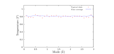
Figure 1: Mode dependence of temperature ($\bar{k}^{2}=\sum_{i=1}^{3}\sin^{2}\left(2\pi\frac{\textbf{ke}_{i}}{N}\right)$)

We remark that the above canonical equilibrium description is in fact a 3D field theory of the initial conditions. As compared to the original action which is four dimensional, we have a dimensionally reduced theory. As a consequence the mass (energy) dimension of the field is $[\Phi]=1/2$. This fact will be used later when we apply dimensional analysis.

In the thermal equilibrium we can perform perturbation theory. Although at large coupling (where we actually performed our simulations) results of perturbation theory are not necessarily perfect, but in several aspects these may “guide the eye” to understand some robust features of the results. The details of perturbation theory in the classical theory can be found in [22]. One uses here two types of propagators

$$G_{ret}(k)=\frac{1}{(k_{0}+i\varepsilon)^{2}-\omega_{k}^{2}},\qquad iG_{3D}(k)=\frac{T}{k_{0}}\,\varrho(k)$$ (11)

where the free spectral function is

$$\varrho(k)=2\pi\mathrm{sgn}(k_{0})\delta(k_{0}^{2}-\omega_{k}^{2}),$$ (12)

and

$$\omega_{k}^{2}=\sum_{i=1}^{3}4\sin^{2}\left(\frac{\pi k_{i}}{N}\right)+m^{2},\qquad k_{i}\in 0\dots N-1.$$ (13)

As a final, technical issue, we remark that solving the field equation corresponds to the pure microcanonical, energy conserving approach to the thermodynamics. However, knowing that the system reaches equilibrium with Boltzmann distribution, we can also use a canonical approach with a heat bath: in the language of the equations of motion it can be realized as a Langevin equation. There we introduce a $\gamma$ damping parameter and a noise represented by $\xi(\mathbf{x})$ independent stochastic variables with uniform distribution at each time step. We then change the update of $\Pi$ to

$$\Pi^{(n)}(\mathbf{x})=(1-\gamma dt)\Pi^{(n-1)}(\mathbf{x})+dt\left(\triangle\Phi^{(n)}(\mathbf{x})-m^{2}\Phi^{(n)}(\mathbf{x})-\frac{\lambda}{6}\left(\Phi^{(n)}(\mathbf{x})\right)^{3}+\xi(\mathbf{x})\right).$$ (14)

This stochastic process drives the system towards an equilibrium distribution with ${\cal P}(E)\sim e^{-\beta E}$ distribution function. Because of the Einstein relation $2\gamma T=\langle{\xi\xi}\rangle$ we can control the temperature of the thermal distribution. This algorithm can largely speed up the thermalization. After the system arrived at the equilibrium, we switched off the noise and damping terms in order that it does not influence the measurements.

4 Equilibrium observables

After we reached the equilibrium state, we can measure expectation values using time average

$$\left\langle A(\Phi,\Pi)\right\rangle=\frac{1}{t}\int\limits_{t_{0}}^{t_{0}+t}\!dt^{\prime}A(\Phi(t),\Pi(t)).$$ (15)

The equilibrium system can be characterized by a single value, for example the temperature.

4.1 Energy

We measured the relation between the temperature and the energy density, the results are shown in Fig. 2.. We found that the relation is linear, with slightly different slope in the symmetric and SSB regimes.

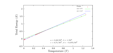
Figure 2: Temperature dependence of total energy ($N^{3}=V=50^{3}$), $\lambda=5$, $m^{2}=-0.5$

One can clearly identify the phase transition region. Since our goal was not to study the phase transition point very accurately, we did not try to focus on this regime close enough to be able to tell details about it.

This figure tells us that the heat capacity is proportional to the number of modes, as it is expected from a classical theory. Rewriting the lattice spacing $a$, this also means that the specific heat is proportional to $a^{3}$. This is the well known Rayleigh instability (ultraviolet catastrophe) of the classical plasma. To have physically meaningful result, the lattice spacing must have a finite value.

4.2 Mass and symmetry breaking

It is important to notice, that the mass parameter of the Lagrangian (the bare mass) is not the same as the mass appearing in the observables (the effective mass). Physically it happens because of the nontrivial effect of the fluctuations.

To estimate this effect (cf. Refs. [26, 27]) we used background field method. We shifted the classical field with its expectation value: $\Phi\to\Phi_{0}+\varphi$, where $\left\langle\varphi\right\rangle=0$. The shifted Lagrangian reads

$${\cal L}= -\frac{m^{2}}{2}\bar{\Phi}^{2}-\frac{\lambda}{24}\bar{\Phi}^{4}-\varphi\left(m^{2}\bar{\Phi}+\frac{\lambda}{6}\bar{\Phi}^{3}\right)+\frac{1}{2}\varphi(-d^{2}-m^{2})\varphi-\frac{\lambda}{4}\bar{\Phi}^{2}\varphi^{2}-$$ (16)

$$-\frac{\lambda}{6}\bar{\Phi}\varphi^{3}-\frac{\lambda}{24}\varphi^{4}.$$

To lowest order (Hartree approximation) we substitute the fluctuations by their expectation values. Using the fact that $\left\langle{\varphi}\right\rangle=0$ we find up to a constant

$${\cal L}=-\frac{1}{2}\left(m^{2}+\frac{\lambda}{2}\left\langle{\varphi^{2}}\right\rangle\right)\bar{\Phi}^{2}-\frac{\lambda}{24}\bar{\Phi}^{4}.$$ (17)

This means that the effective mass is modified by the effect of the fluctuations. Since the mass dimension of the field is $[\varphi]={1/2}$, by dimensional reasons $\left\langle{\varphi^{2}}\right\rangle\sim T$. On the other hand this is a correction to the mass squared, and so the coefficient is also dimensionful, with finite lattice spacing it is proportional to $a^{-1}$. The coefficient in leading order in perturbation theory reads

$$\left\langle{\varphi^{2}}\right\rangle=\frac{T}{N^{3}}\sum\limits_{k\in\bar{U}}\frac{1}{\sum_{i=1}^{3}4\sin^{2}\left(\frac{\pi k_{i}}{N}\right)+m^{2}}\stackrel{{\scriptstyle N\to\infty}}{{\longrightarrow}}0.2527T-\frac{mT}{4\pi}+{\cal O}(m^{2}),$$ (18)

but this number is unreliable for large couplings.

One consequence of this formula is that at fixed negative bare mass the effective mass term will be positive at high enough temperature. This means that the minimum of the effective action for the constant field (the constrained free energy) will become zero at this temperature: the symmetry is restored. To see it we measured the expectation value of the field for various tree level masses at different temperatures. The result can be seen on Fig. 3.

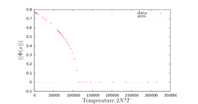
Figure 3: Temperature dependence of the expectation value of the field.

A more delicate question is that in the 3D classical field theory, unlike in the 4-dimensional theory, the temperature influences the renormalization. This means that the meaning of mass and temperature cannot be separated from each other in that clear way as it can be done in the 4D case. We therefore also performed simulations with fixed effective mass at different temperatures: this requires to tune the bare mass parameter. In practice we fix the desired effective mass and the bare mass, and tune the temperature accordingly with the application of Langevin equations described earlier.

For the definition of the mass we measured the correlation function

$$G(t,\textbf{x}):=\langle\Phi(t,\textbf{x})\Phi(0)\rangle$$ (19)

In leading order of perturbation theory we expect that this correlator is the free one, where we should also take into account the mass modification:

$$G(t,\textbf{k})=\left\langle|\Phi_{k}|^{2}\right\rangle\cos\omega_{k}t,$$ (20)

where $\omega_{k}^{2}=\textbf{k}^{2}+m^{2}+\frac{\lambda}{2}\left\langle{\varphi^{2}}\right\rangle$. If one goes beyond the first order of perturbation theory, then one obtains self-energy corrections, and the pure harmonic behavior of the correlator will be spoiled. If a one-particle particle mass shell is dominant, then we can speak about quasiparticle excitations. In that case in real time evolution one can observe a damped oscillation

$$G(t,\textbf{k})\sim\exp(-t/\tau_{k})\cos(\omega_{k}t).$$ (21)

However, the closer we are to the phase transition point, the worse behavior could be observed for the static $\Phi$ field, as it is demonstrated in Fig. 4.

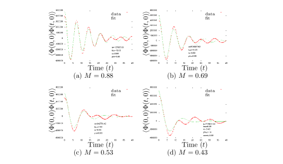
Figure 4: The real time behavior of the field correlation function at different bare masses, $\lambda=5$.

We can see that far from the phase transition point, where the effective mass is large, the quasiparticle assumption is valid. With decreasing effective mass the fit works worse and worse. In this case the definition of the notion “mass” is not unique anymore. For a more sophisticated description we should use the complete spectral function; but we just need a characterization of the mass and temperature. For that purpose we use the best quasiparticle fit to the real time data for the zero mode. This is some mean value of the spectral peak, in the vicinity of the phase transition point it remains finite, as opposed to the inverse spatial correlation length.

The temperature dependence of the so-defined mass is shown in Fig. 5 with fixed bare mass $m^{2}=-0.5$. We can clearly see the position of the phase transition point which sits at the minimum of this curve.

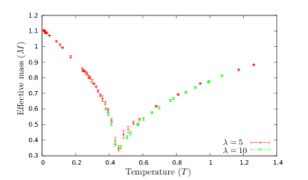
Figure 5: Temperature dependence of the effective mass parameter for various interaction strength ($\lambda$) where $m^{2}=-0.5$. It has a minimum at the phase transition point, but with our definition the minimum is not at zero.

One may also check, whether we reached the infinite volume (thermodynamical) limit. For that we determined the temperature dependence of the mass at various volumes, see left panel of Fig. 6. This plot suggests that we reached already the thermodynamical limit. We can also check the temperature dependence of the effective mass, this is shown in the right panel of Fig. 6. We see that for different bare masses the effective mass values sit on a unique curve.

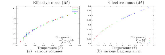
Figure 6: Left panel: effective mass at different volumes. Right panel: effective mass in theories with different bare mass.

5 Viscosity

The central topic of this paper is the determination of the shear viscosity. The Kubo-formula for momentum transport [1] requires to compute

$$\eta=\lim_{\omega\rightarrow 0}\frac{\varrho_{T_{12}T_{21}}(\omega,\textbf{k}=0)}{\omega},$$ (22)

where

$$\varrho_{AB}(x)=\langle\left[A(x),B(0)\right]\rangle,$$ (23)

$\eta$ is the shear-viscosity and $T_{12}$ is the $12$ component of the energy momentum tensor; in case of the scalar field theory it is $T_{12}=\partial_{1}\Phi\partial_{2}\Phi$. In classical theory we cannot measure the commutator of two operators, but we can measure the correlation function instead. For $A(x)$ and $B(0)$ operators it is defined as

$$S_{AB}(x)=\langle A(x)B(0)\rangle_{cl},$$ (24)

where the “cl” subscript refers to the classical correlation function. To connect this quantity with the viscosity we use the Green-Kubo formula, which claims that

$$\varrho_{AB,cl}(\omega,\mathbf{k})=\beta\omega S_{AB,cl}(\omega,\mathbf{k}),$$ (25)

which is a direct consequence of the quantum Kubo-Martin-Schwinger relation

$$\varrho_{AB}(\omega,\mathbf{k})=(1-e^{-\beta\omega})S_{AB,cl}(\omega,\mathbf{k}),$$ (26)

in the $\beta\omega\to 0$ limit. Using this relation the viscosity is

$$\eta_{cl}=\beta S_{T_{12}T_{12}}(k=0).$$ (27)

The direct result of our simulations in real time can be seen in Fig. 7. We repeated the measurements of $S_{T_{12}T_{12}}$ for five different configurations, meaning that after each measurement we allowed the system evolve in time until we reached an independent configuration. This makes it possible to estimate the statistical error of the simulation.

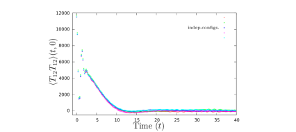
Figure 7: $T_{12}$ autocorrelation function in real time.

The relevant information, the transport-peak can be extracted from the Fourier-transformed data shown in Fig. 8. To understand what we see in this figure we recall that in the leading order of perturbation theory we expect a branch cut starting at $2m$, and a Dirac-delta peak at $k=0$, just like in the Fourier transform of $\langle{\Phi^{2}(x)\Phi^{2}(0)}\rangle$. The higher order terms result in the smearing of the cut and the Dirac-delta peak as well, the former yielding a broad bump, the latter leading to the transport peak. The desired result is the height of this peak at $\omega=0$.

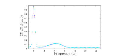
Figure 8: $T_{12}$ correlator in frequency space.

One can repeat this measurement at different temperatures as well, this can be seen on Fig. 9. This figure suggests that the classical shear viscosity depends more or less linearly on the temperature. It also follows from dimensional analysis: since $[\Phi]=1/2$ is the mass dimension of the field, $[T_{12}]\sim 3$, its correlator has $6$th power of energy dimension. After Fourier transformation there remains $2$, and after division by the temperature, there remains $1$, a linear energy dependence. Since the main source of energy dependence in the classical case is the temperature, we expect proportionality with $T$.

To verify numerically this, we also present the $\eta_{cl}/T$ curve in Fig. 10. We see that the ratio is approximately constant, but with an enhanced behavior near the critical point. This figure suggests that the classical viscosity, just like other susceptibilities, shows a critical behavior, exhibiting a peak at the phase transition point.

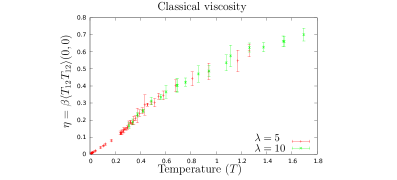
Figure 9: Temperature dependence of the classical shear-viscosity.

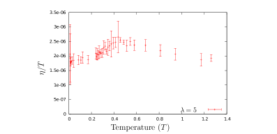
Figure 10: Classical shear viscosity over temperature as a function of the temperature. The enhanced behavior is around the phase transition point, suggesting that the viscosity also shows a critical behavior.

5.1 Interpretation

One can compute the classical viscosity in perturbation theory to leading order, similarly what was done in Ref. [30]. With point splitting we can write

$$S(x)=\left\langle{T_{12}(x)T_{12}(0)}\right\rangle =\lim\limits_{{x^{\prime}\to x}\atop{y^{\prime}\to y\to 0}}\partial_{x1}\partial_{x^{\prime}1}\partial_{y1}\partial_{y^{\prime}1}\left\langle{\Phi(x)\Phi(x^{\prime})\Phi(y)\Phi(y^{\prime})}\right\rangle=$$ (28)

$$=\partial_{1}^{2}iG_{3D}(x)\partial_{2}^{2}iG_{3D}(x)+(\partial_{1}\partial_{2}iG_{3D}(x))^{2}.$$

After Fourier transformation we have

$$S(p) =\int\frac{d^{4}k}{(2\pi)^{4}}\left[k_{1}^{2}(p-k)_{2}^{2}+k_{1}k_{2}(p-k)_{1}(p-k)_{2}\right]iG_{3D}(k)iG_{3D}(p-k)=$$ (29)

$$=T^{2}\int\frac{d^{4}k}{(2\pi)^{2}}\frac{k_{1}^{2}(p-k)_{2}^{2}+k_{1}k_{2}(p-k)_{1}(p-k)_{2}}{k_{0}(p_{0}-k_{0})}\varrho(k)\varrho(p-k).$$

This is very similar to the $\Phi^{2}\Phi^{2}$ correlation function discussed in [30], and also very similar to the discontinuity of the quantum version of it.

To proceed we use the Green-Kubo relation (27) to write

$$\eta_{cl}=2T\int\!\frac{d^{4}k}{(2\pi)^{4}}\,\frac{k_{1}^{2}k_{2}^{2}}{k_{0}^{2}}\varrho^{2}(k).$$ (30)

Evaluating this expression with the free spectral function (12) we obtain infinity: this means that for free theories the viscosity, like all other transport coefficient, is infinite. We can apply a Breit-Wigner approximation for the spectral function

$$\varrho(k)=\frac{4k_{0}\gamma_{k}}{(k_{0}^{2}-\omega_{k})^{2}+4k_{0}^{2}\gamma_{k}^{2}},$$ (31)

then we can approximate for small width and for $k_{0}>0$:

$$\varrho^{2}(k)\approx\frac{2\pi}{\gamma_{k}\omega_{k}^{2}}\delta(k_{0}-\omega_{k}).$$ (32)

This leads to

$$\eta_{cl}=4T\int\!\frac{d^{3}\mathbf{k}}{(2\pi)^{3}}\,\frac{k_{1}^{2}k_{2}^{2}}{\gamma_{k}\omega_{k}^{4}}.$$ (33)

This integral is still divergent in the continuum limit. The leading contribution comes from large momenta. The asymptotics of $\gamma_{k}\omega_{k}$ has been found in [30] (see also [24]), it is $\frac{\lambda^{2}T^{2}}{384\pi}$. In the remaining $\omega_{k}^{-3}$ factor one can put $m=0$. Therefore to leading order we have

$$\eta_{cl}=\frac{1536\pi}{\lambda^{2}T}\int\!\frac{d^{3}\mathbf{k}}{(2\pi)^{3}}\,\frac{k_{1}^{2}k_{2}^{2}}{(k_{1}^{2}+k_{2}^{2}+k_{3}^{2})^{3/2}}+\dots.$$ (34)

Rewriting this integral in terms of the dimensionless momenta $ka$, and integrating it in the Brillouin zone $-\pi<ka<\pi$, one finds

$$\eta_{cl}=\frac{\eta_{lat}}{a^{4}},\qquad\eta_{lat}=\frac{321.3\pi}{\lambda^{2}T}+\dots.$$ (35)

The fact that $\eta_{cl}\sim a^{-4}$ is consistent with the results of [30] for the $\Phi^{2}$ autocorrelation function. There a logarithmic divergence was found, therefore the energy-momentum tensor correlation function, which has two derivatives more than $\Phi^{2}$, should scale as $a^{-4}$.

Although this result is just a first order perturbative estimate, the robust part of the result is that the classical shear viscosity is proportional to $a^{-4}$. After determining $\eta_{lat}$ by lattice simulations, this is the way how one can recover the classical value of the viscosity.

The next question is how can one relate $\eta_{cl}$ to the shear viscosity of quantum systems. The facit of the comparison of the classical and quantum calculations [30, 33] was that the perturbative quantum result was rather close to the classical one, if one chooses a cutoff $\Lambda\sim T$. The exact value of the coefficient is not known to be universal, probably it depends on the quantity in question. But, up to a constant, we can estimate the result of the full quantum result by setting $\eta\sim(aT)^{4}\eta_{cl}$. If we measure the shear viscosity from the lattice, we have

$$\eta\sim T^{4}\eta_{lat}.$$ (36)

Below we will use unity for the proportionality constant.

Of course, this formula is based on the assumption that the quantum result is dominated by the classical fields. Also, unfortunately, we do not know the coefficient in this formula, nevertheless, we can give a temperature profile of the $\eta/s$ ratio.

The entropy density of the quantum system is poorly approximated by the classical modes, so we use for the $\eta/s$ estimate the entropy density of a free one component gas with

$$s=\int\!\frac{d^{3}\mathbf{k}}{(2\pi)^{3}}\,\left[\frac{\omega_{k}}{e^{\beta\omega_{k}}-1}-\ln(1-e^{-\beta\omega_{k}})\right].$$ (37)

Here $\omega_{k}^{2}=\mathbf{k}^{2}+m_{eff}^{2}$, where $m_{eff}$ was taken from the classical simulations. In this way we can present our estimate for the $\eta/s$ ratio in Fig. 11.

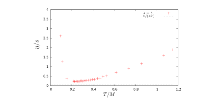
Figure 11: The quantum $\eta/s$ estimated by the classical $\Phi^{4}$ theory, using $a=T^{-1}$ lattice spacing.

We see a curve typical for the behavior of the shear viscosity in any matter near the phase transition point. For a qualitative comparison we show the $\eta/s$ ratio for QCD [34] in Fig. 12 versus our results that was rescaled to fit to the high temperature part.

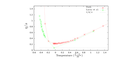
Figure 12: Qualitative comparison of $\eta/s$ of QCD plasma and the classical $\Phi^{4}$ theory, after rescaling. The QCD data are taken from [34].

6 Summary

In this work we used numerical simulations of the quartic classical field theory to give an estimate for the shear viscosity. To this end we solved the discretized classical equations of motion. This leads to thermalization, where one can determine the expectation value of different observables by time averaging. We first determined the field autocorrelation function, and analyzed it by assuming quasiparticle behavior. Then we measured the correlator of the $12$ component of the energy-momentum tensor. Using the Green-Kubo formula this quantity is proportional to the shear viscosity. The shear viscosity $\eta_{lat}$ was found to depend approximately linearly on $T$ which was expected by classical dimensional analysis. This behaviour was superimposed by a characteristic critical behavior near the phase transition regime. Finally we pointed out that the classical viscosity comes from the lattice viscosity as $\eta_{cl}=\eta_{lat}a^{-4}$ where $a$ is the lattice spacing. Translating the classical result into the shear viscosity of the quantum system, we argued that $a^{-1}\sim T$ is the correct choice, but the proportionality constant is not known. This allows us to make an estimate also on the temperature profile of $\eta/s$, which turns out to be rather similar to the result of QCD near the critical region.

As future prospects we plan to repeat this analysis to other models including gauge theories. Another interesting extension could be to study the effects of the quantum corrections to the equations of motion. This could give a hint on the reliability of the classical estimate.

References

- [1] A. Hosoya, M. a. Sakagami and M. Takao, Annals Phys. 154, 229 (1984).
- [2] S. Jeon, Phys. Rev. D 52, 3591 (1995) [hep-ph/9409250].
- [3] S. Jeon and L. G. Yaffe, Phys. Rev. D 53, 5799 (1996) [hep-ph/9512263].
- [4] A. Jakovac, Phys. Rev. D 65, 085029 (2002) [hep-ph/0112188].
- [5] P. B. Arnold, G. D. Moore and L. G. Yaffe, JHEP 0011, 001 (2000) [hep-ph/0010177].
- [6] P. B. Arnold, G. D. Moore and L. G. Yaffe, JHEP 0305, 051 (2003) [hep-ph/0302165].
- [7] A. Dobado and F. J. Llanes-Estrada, Phys. Rev. D 69, 116004 (2004) [hep-ph/0309324].
- [8] M. Buballa, K. Heckmann and J. Wambach, Prog. Part. Nucl. Phys. 67, 348 (2012) [arXiv:1202.0724 [hep-ph]].
- [9] S. Mitra and S. Sarkar, Phys. Rev. D 87, no. 9, 094026 (2013) [arXiv:1303.6408 [hep-ph]].
- [10] Z. Xu and C. Greiner, Phys. Rev. C 71, 064901 (2005) [hep-ph/0406278].
- [11] Z. Xu and C. Greiner, Phys. Rev. C 76, 024911 (2007) [hep-ph/0703233].
- [12] G. Aarts and J. M. Martinez Resco, JHEP 0402, 061 (2004) [hep-ph/0402192].
- [13] A. Peshier and W. Cassing, Phys. Rev. Lett. 94, 172301 (2005) [hep-ph/0502138].
- [14] S. S. Adler et al. [PHENIX Collaboration], Phys. Rev. Lett. 91, 182301 (2003) [nucl-ex/0305013].
- [15] J. Liao and V. Koch, Phys. Rev. C 81, 014902 (2010) [arXiv:0909.3105 [hep-ph]].
- [16] H. B. Meyer, Phys. Rev. D 76, 101701 (2007) [arXiv:0704.1801 [hep-lat]].
- [17] P. Petreczky, J. Phys. G 35, 044033 (2008) [arXiv:0710.5561 [nucl-th]].
- [18] P. Kovtun, D. T. Son and A. O. Starinets, JHEP 0310, 064 (2003) [hep-th/0309213].
- [19] P. Kovtun, D. T. Son and A. O. Starinets, Phys. Rev. Lett. 94, 111601 (2005) [hep-th/0405231].
- [20] G. Aarts and J. Smit, Phys. Lett. B 393, 395 (1997) [hep-ph/9610415].
- [21] B. J. Nauta and C. G. van Weert, Phys. Lett. B 444, 463 (1998) [hep-ph/9709401].
- [22] W. Buchmuller and A. Jakovac, Phys. Lett. B 407, 39 (1997) [hep-ph/9705452].
- [23] W. Buchmuller and A. Jakovac, Nucl. Phys. B 521, 219 (1998) [hep-th/9712093].
- [24] G. Aarts and J. Berges, Phys. Rev. Lett. 88, 041603 (2002) [hep-ph/0107129].
- [25] B. Holdom, J. Phys. A 39, 7485 (2006) [hep-th/0602236].
- [26] S. Borsanyi, A. Patkos and D. Sexty, Phys. Rev. D 66, 025014 (2002) [hep-ph/0203133].
- [27] S. Borsanyi, A. Patkos and D. Sexty, Phys. Rev. D 68, 063512 (2003) [hep-ph/0303147].
- [28] D. Boyanovsky, C. Destri and H. J. de Vega, Phys. Rev. D 69, 045003 (2004) [hep-ph/0306124].
- [29] J. Berges, B. Schenke, S. Schlichting and R. Venugopalan, Nucl. Phys. A 931, 348 (2014) [arXiv:1409.1638 [hep-ph]].
- [30] A. Jakovac, Phys. Lett. B 446, 203 (1999) [hep-ph/9808349].
- [31] M. Le Bellac, Thermal Field Theory (Cambridge University Press, 1996)
-
[32]
www.fftw.org - [33] E. k. Wang, U. W. Heinz and X. f. Zhang, Phys. Rev. D 53, 5978 (1996) [hep-ph/9509331].
- [34] R. A. Lacey, N. N. Ajitanand, J. M. Alexander, P. Chung, W. G. Holzmann, M. Issah, A. Taranenko and P. Danielewicz et al., Phys. Rev. Lett. 98, 092301 (2007) [nucl-ex/0609025].