On a linear partial differential equation of the higher order in two variables with initial condition whose coefficients are real-valued simple step functions

Abstract

By using the method developed in the paper [Georg. Inter. J. Sci. Tech., Volume 3, Issue 1 (2011), 107-129], it is obtained a representation in an explicit form of the weak solution of a linear partial differential equation of the higher order in two variables with initial condition whose coefficients are real-valued simple step functions

2000 Mathematics Subject Classification: Primary 34Axx ; Secondary 34A35, 34K06.

Key words and phrases: linear partial differential equation of the higher order in two variables, Fourier differential operator.

1. Introduction

In [5] has been obtained a representation in an explicit form of the solution of the linear partial differential equation of the higher order in two variables with initial condition whose coefficients were real-valued coefficients. The aim of the present manuscript is resolve an analogous problem for a linear partial differential equation of the higher order in two variables with initial condition whose coefficients are real-valued simple step functions.

The paper is organized as follows.

In Section 2, we consider some auxiliary results obtained in the paper [5]. In Section 3, it is obtained a representation in an explicit form of the weak solution of the partial differential equation of the higher order in two variables with initial condition whose coefficients are real-valued simple step functions.

2. Some auxiliary results

Definition 2.1.

Fourier differential operator $(\mathcal{F}){\frac{\partial}{\partial x}}$ in $R^{\infty}$ is defined as follows :

$$(\mathcal{F}){\frac{\partial}{\partial x}}\begin{pmatrix}\frac{a_{0}}{2}\\ a_{1}\\ b_{1}\\ a_{2}\\ b_{2}\\ a_{3}\\ b_{3}\\ \vdots\end{pmatrix}=\begin{pmatrix}0&0&0&0&0&0&0&\dots&\\ 0&0&\frac{1\pi}{l}&0&0&0&0&\dots&\\ 0&-\frac{1\pi}{l}&0&0&0&0&0&\dots&\\ 0&0&0&0&\frac{2\pi}{l}&0&0&\dots&\\ 0&0&0&-\frac{2\pi}{l}&0&0&0&\dots&\\ 0&0&0&0&0&0&\frac{3\pi}{l}&\ddots&\\ 0&0&0&0&0&-\frac{3\pi}{l}&0&\ddots&\\ \vdots&\vdots&\vdots&\vdots&\vdots&\vdots&\ddots&\ddots&\end{pmatrix}\times\begin{pmatrix}\frac{a_{0}}{2}\\ a_{1}\\ b_{1}\\ a_{2}\\ b_{2}\\ a_{3}\\ b_{2}\\ \vdots\end{pmatrix}.$$

For $n\in\mathbb{N}$, let $FD^{n}[-l,l[$ be a vector space of all $n$-times differentiable functions on $[-l,l[$ such that for arbitrary $0\leq k\leq n-1$, a series obtained by a differentiation term by term of the Fourier series of $f^{(k)}$ pointwise converges to $f^{(k+1)}$ for all $x\in[-l,l[$.

Lemma 2.2.

Let $f\in FD^{(1)}[-l,l[$. Let $G_{M}$ be an embedding of the $FD^{(1)}[-l,l[$ in to $R^{\infty}$ which sends a function to a sequence of real numbers consisting from its Fourier coefficients. i.e., if

$$f(x)=\frac{c_{0}}{2}+\sum_{k=1}^{\infty}c_{k}\cos(\frac{k\pi x}{l})+d_{k}\sin(\frac{k\pi x}{l})~{}(x\in[-l,l[),$$

then $G_{F}(f)=(\frac{c_{0}}{2},c_{1},d_{1},c_{2},d_{2},\dots)$. Then, for $f\in FD^{(1)}[-l,l[$, the following equality

$$\Big{(}G_{F}^{-1}\circ(\mathcal{F}){\frac{\partial}{\partial x}}\circ G_{F}\Big{)}(f)=\frac{\partial}{\partial x}(f)$$

holds.

Proof.

Assume that for $f\in FD^{(1)}[-l,l[$, we have the following representation

$$f(x)=\frac{c_{0}}{2}+\sum_{k=1}^{\infty}c_{k}\cos\Big{(}\frac{k\pi x}{l}\Big{)}+d_{k}\sin\Big{(}\frac{k\pi x}{l}\Big{)}~{}(x\in[-l,l[).$$

By the definition of the class $FD^{(1)}[-l,l[$, we have

$$\frac{d}{dx}(f)=\frac{\partial}{\partial x}(\frac{c_{0}}{2}+\sum_{k=1}^{\infty}c_{k}\cos\Big{(}\frac{k\pi x}{l}\Big{)}+d_{k}\sin\Big{(}\frac{k\pi x}{l}\Big{)})=$$

$$\sum_{k=1}^{\infty}c_{k}\frac{\partial}{\partial x}(\cos\Big{(}\frac{k\pi x}{l}\Big{)})+d_{k}\frac{\partial}{\partial x}(\sin\Big{(}\frac{k\pi x}{l}\Big{)})=$$

$$\sum_{k=1}^{\infty}-c_{k}\frac{k\pi}{l}\sin\Big{(}\frac{k\pi x}{l}\Big{)}+d_{k}\frac{k\pi}{l}\cos\Big{(}\frac{k\pi x}{l}\Big{)}=$$

$$\sum_{k=1}^{\infty}\frac{k\pi d_{k}}{l}\cos\Big{(}\frac{k\pi x}{l}\Big{)}-\frac{k\pi c_{k}}{l}\sin\Big{(}\frac{k\pi x}{l}\Big{)}.$$

By the definition of the composition of mappings, we have

$$\Big{(}G_{F}^{-1}\circ(\mathcal{F}){\frac{\partial}{\partial x}}\circ G_{F}\Big{)}(f)=G_{F}^{-1}((\mathcal{F}){\frac{\partial}{\partial x}}((G_{F}(f))))=G_{F}^{-1}((\mathcal{F}){\frac{\partial}{\partial x}}\begin{pmatrix}\frac{c_{0}}{2}\\ c_{1}\\ d_{1}\\ c_{2}\\ d_{2}\\ c_{3}\\ d_{3}\\ \vdots\end{pmatrix})=$$

$$G_{F}^{-1}(\begin{pmatrix}0&0&0&0&0&0&0&\dots&\\ 0&0&\frac{1\pi}{l}&0&0&0&0&\dots&\\ 0&-\frac{1\pi}{l}&0&0&0&0&0&\dots&\\ 0&0&0&0&\frac{2\pi}{l}&0&0&\dots&\\ 0&0&0&-\frac{2\pi}{l}&0&0&0&\dots&\\ 0&0&0&0&0&0&\frac{3\pi}{l}&\ddots&\\ 0&0&0&0&0&-\frac{3\pi}{l}&0&\ddots&\\ \vdots&\vdots&\vdots&\vdots&\vdots&\vdots&\ddots&\ddots&\end{pmatrix}\times\begin{pmatrix}\frac{c_{0}}{2}\\ c_{1}\\ d_{1}\\ c_{2}\\ d_{2}\\ c_{3}\\ d_{3}\\ \vdots\end{pmatrix})=$$

$$G_{F}^{-1}(\begin{pmatrix}0\\ \frac{1\pi d_{1}}{l}\\ -\frac{1\pi c_{1}}{l}\\ \frac{2\pi d_{2}}{l}\\ -\frac{2\pi c_{2}}{l}\\ \frac{3\pi d_{3}}{l}\\ -\frac{3\pi c_{3}}{l}\\ \vdots\end{pmatrix})=\sum_{k=1}^{\infty}\frac{k\pi d_{k}}{l}\cos\Big{(}\frac{k\pi x}{l}\Big{)}-\frac{k\pi c_{k}}{l}\sin\Big{(}\frac{k\pi x}{l}\Big{)}.$$

∎

By the scheme used in the proof of Lemma 2.1, we can get the validity of the following assertion.

Lemma 2.3.

Let $G_{M}$ be an embedding of the $FD^{n}[-l,l[$ in to $R^{\infty}$ which sends a function to a sequence of real numbers consisting from its Fourier coefficients.

Then, for $f\in FD^{(n)}[-l,l[$ and $A_{k}\in R(0\leq k\leq n)$, the following equality

$$\Big{(}G_{F}^{-1}\circ\Big{(}\sum_{k=0}^{n}A_{k}((\mathcal{F}){\frac{\partial}{\partial x}})^{k}\Big{)}\circ G_{F}\Big{)}(f)=\sum_{k=0}^{n}a_{k}\frac{\partial^{k}}{\partial x^{k}}(f)$$

holds.

Example 2.4.

[3] If $A$ is the real matrix

$$\begin{pmatrix}\sigma&\omega&\\ -\omega&\sigma&\end{pmatrix},$$

then

$$e^{tA}=e^{\sigma t}\begin{pmatrix}\cos(\omega t)&\sin(\omega t)&\\ -\sin(\omega t)&\cos(\omega t)&\end{pmatrix}.$$

Lemma 2.5.

For $m\geq 1$, let us consider a linear autonomous nonhomogeneous ordinary differential equations of the first order

$${\frac{d}{dt}}((a_{k})_{k\in\mathbb{N}})=\Big{(}\sum_{n=0}^{2m}A_{n}\Big{(}(\mathcal{F})\frac{\partial}{\partial x}\Big{)}^{n}\Big{)}\times((a_{k})_{k\in\mathbb{N}})+(f_{k})_{k\in\mathbb{N}}$$

with initial condition

$$(a_{k}(0))_{k\in\mathbb{N}}=(C_{k})_{k\in\mathbb{N}},$$

where

$(i)$ $(C_{k})_{k\in\mathbb{N}}\in{\bf R}^{\infty}$;

$(ii)$ $f=(f_{k})_{k\in\mathbb{N}}$ is the sequence of continuous functions of a parameter $t$ on $R$.

For each $k\geq 1$, we put

$$\sigma_{k}=\sum_{n=0}^{m}(-1)^{n}A_{2n}(\frac{k\pi}{l})^{2n},$$

$$\omega_{k}=\sum_{n=0}^{m-1}(-1)^{n}A_{2n+1}(\frac{k\pi}{l})^{2n+1}.$$

Then the solution of (2.6)-(2.7) is given by

$$(a_{k}(t))_{k\in\mathbb{N}}=e^{t(\sum_{n=0}^{2m}A_{n}\Big{(}(\mathcal{F})\frac{\partial}{\partial x}\Big{)}^{n})}\times(C_{k})_{k\in\mathbb{N}}+\int_{0}^{t}e^{(\tau-t)(\sum_{n=0}^{2m}A_{n}\Big{(}(\mathcal{F})\frac{\partial}{\partial x}\Big{)}^{n})}\times f(\tau)d\tau,$$

where $e^{t((\sum_{n=0}^{2m}A_{n}\Big{(}(\mathcal{F})\frac{\partial}{\partial x}\Big{)}^{n})}$ denotes an exponent of the matrix $t(\sum_{n=0}^{2m}A_{n}\Big{(}(\mathcal{F})\frac{\partial}{\partial x}\Big{)}^{n})$ and it exactly coincides with an infinite-dimensional $(1,2,2,\dots)$ -cellular matrix $D(t)$ with cells $(D_{k}(t))_{k\in\mathbb{N}}$ for which $D_{0}(t)=(e^{tA_{0}})$ and

$$D_{k}(t)=e^{\sigma_{k}t}\begin{pmatrix}\cos(\omega_{k}t)&\sin(\omega_{k}t)&\\ -\sin(\omega_{k}t)&\cos(\omega_{k}t)&\end{pmatrix},$$

where for $k\geq 1$, $\sigma_{k}$ and $\omega_{k}$ are defined by (2.8)-(2.9), respectively.

Proof.

We know that if we have a linear autonomous inhomogeneous ordinary differential equations of the first order

$${\frac{d}{dt}}((a_{k})_{k\in\mathbb{N}})=E\times((a_{k})_{k\in N})+(f_{k})_{k\in\mathbb{N}}$$

with initial condition

$$(a_{k}(0))_{k\in\mathbb{N}}=(C_{k})_{k\in\mathbb{N}},$$

where

$(i)$ $(C_{k})_{k\in\mathbb{N}}\in{\bf R}^{\infty}$;

$(ii)$ $(f_{k}))_{k\in\mathbb{N}}$ is the sequence of continuous functions of parameter $t$ on $R$;

$(iii)$ $E$ is an infinite dimensional $(1,2,2,\dots)$-cellular matrix with cells $(E_{k})_{k\in\mathbb{N}}$.

Then the solution of (2.6)-(2.7) is given by (cf. [3], §6, Section 1)

$$(a_{k}(t))_{k\in\mathbb{N}}=e^{tE}\times(C_{k})_{k\in\mathbb{N}}+\int_{0}^{t}e^{(\tau-t)E}\times f(\tau)d\tau,$$

where $e^{tE}$ and $e^{(\tau-t)E}$ denote exponents of matrices $tE$ and $(\tau-t)E$, respectively.

Note that $t\sum_{n=0}^{2m}A_{n}\Big{(}(\mathcal{F})\frac{\partial}{\partial x}\Big{)}^{n}$ is an infinite-dimensional $(1,2,2,\dots)$-cellular matrix with cells $(tE_{k})_{k\in\mathbb{N}}$ such that $tE_{0}=(tA_{0})$ and

$$tE_{k}=\begin{pmatrix}t\sigma_{k}&t\omega_{k}&\\ -t\omega_{k}&t\sigma_{k}&\end{pmatrix}$$

for $k\geq 1$. Under notations (2.8)-(2.9), by using Example 2.4 we get that for $t\in R$, $e^{tE}$ exactly coincides with an infinite-dimensional $(1,2,2,\dots)$ -cellular matrix $D(t)$ with cells $(D_{k}(t))_{k\in\mathbb{N}}$ for which $D_{0}(t)=(e^{tA_{0}})$ and

$$D_{k}(t)=e^{\sigma_{k}t}\begin{pmatrix}\cos(\omega_{k}t)&\sin(\omega_{k}t)&\\ -\sin(\omega_{k}t)&\cos(\omega_{k}t)&\end{pmatrix}.$$

Note that, for $0\leq\tau\leq t$, the matrix $e^{(\tau-t)E}$ exactly coincides with an infinite-dimensional $(1,2,2,\dots)$ -cellular matrix $D(\tau-t)$.

∎

The following proposition is a simple consequence of Lemma 2.5.

Corollary 2.6.

For $m\geq 1$, let us consider a linear partial differential equation

$$\frac{\partial}{\partial t}\Psi(t,x)=\sum_{n=0}^{2m}A_{n}\frac{\partial^{n}}{\partial x^{n}}\Psi(t,x)~{}((t,x)\in[0,+\infty[\times[-l,l[)$$

with initial condition

$$\Psi(0,x)=\frac{c_{0}}{2}+\sum_{k=1}^{\infty}c_{k}\cos\Big{(}\frac{k\pi x}{l}\Big{)}+d_{k}\sin\Big{(}\frac{k\pi x}{l}\Big{)}\in FD^{(0)}[-l,l[.$$

If $(\frac{c_{0}}{2},c_{1},d_{1},c_{2},d_{2},\dots)$ is such a sequence of real numbers that a series $\Psi(t,x)$ defined by

$$\Psi(t,x)=\frac{e^{tA_{0}}c_{0}}{2}+\sum_{k=1}^{\infty}e^{\sigma_{k}t}\Big{(}(c_{k}\cos(\omega_{k}t)+$$

$$d_{k}\sin(\omega_{k}t))\cos(\frac{k\pi x}{l})+(d_{k}\cos(\omega_{k}t)-c_{k}\sin(\omega_{k}t))\sin(\frac{k\pi x}{l})\Big{)}$$

belongs to the class $FD^{(2m)}[-l,l[$ as a series of a variable $x$ for all $t\geq 0$, and is differentiable term by term as a series of a variable $t$ for all $x\in[-l,l[$, then $\Psi$ is a solution of $(2.17)$-$(2.18)$.

3. Solution of a linear partial differential equation of the higher order in two variables with initial condition when coefficients are real-valued simple step functions

Let $0=t_{0}<\cdots<t_{I}=T$ and $-l=x_{0}<\cdots<x_{J}=l$. Suppose that

$$A_{n}(t,x)=\sum_{i=0}^{I-1}\sum_{j=0}^{J-1}A_{n}^{(i,j)}\times\chi_{[t_{i},t_{i+1}[\times[x_{j},x_{j+1}[}(t,x).$$

For $m\geq 1$, let us consider a partial differential equation

$$\frac{\partial}{\partial t}\Psi(t,x)=\sum_{n=0}^{2m}A_{n}(t,x)\frac{\partial^{n}}{\partial x^{n}}\Psi(t,x)~{}((t,x)\in[0,T[\times[-l,l[)$$

with initial condition

$$\Psi(0,x)=\frac{c_{0}}{2}+\sum_{k=1}^{\infty}c_{k}\cos\Big{(}\frac{k\pi x}{l}\Big{)}+d_{k}\sin\Big{(}\frac{k\pi x}{l}\Big{)}\in FD^{(0)}[-l,l[.$$

Definition 3.1.

We say that $\Psi(t,x)$ is a weak solution of (3.1)-(3.2) if the following conditions hold:

(i)  $\Psi(t,x)$ satisfies (3.1) for each $(t,x)\in[0,T[\times[-l,l[$ for which $t\neq t_{i}(0\leq i\leq I)$ or $x\neq x_{j}(0\leq j\leq J)$;

(ii) $\Psi(t,x)$ satisfies (3.2);

(iii)  for each fixed $x\in[-l,l[$, the function $\Psi(t,x)$ is continuous with respect to $t\in[0,T[$, and for each $t\in[0,T[$ the function $\Psi(t,x)$ is continuous with respect to $x$ on $[-l,l[$ except points $\{x_{j}:0\leq j\leq J-1\}$.

First, let fix $j$ and consider a partial differential equation

$$\frac{\partial}{\partial t}\Psi_{(0,j)}(t,x)=\sum_{n=0}^{2m}A^{(0,j)}_{n}(t,x)\frac{\partial^{n}}{\partial x^{n}}\Psi_{(0,j)}(t,x)~{}((t,x)\in[0,+\infty[\times[-l,l[)$$

with initial condition

$$\Psi_{(0,j)}(t_{0},x)=\frac{c_{0}}{2}+\sum_{k=1}^{\infty}c_{k}\cos\Big{(}\frac{k\pi x}{l}\Big{)}+d_{k}\sin\Big{(}\frac{k\pi x}{l}\Big{)}=$$

$$\frac{c^{(0,j)}_{0}}{2}+\sum_{k=1}^{\infty}c^{(0,j)}_{k}\cos\Big{(}\frac{k\pi x}{l}\Big{)}+d^{(0,j)}_{k}\sin\Big{(}\frac{k\pi x}{l}\Big{)}\in FD^{(0)}[-l,l[,$$

By Corollary 2.6, under some restrictions on $(\frac{c_{0}}{2},c_{1},d_{1},c_{2},d_{2},\dots)$, a series $\Psi_{(0,j)}(t,x)$ defined by

$$\Psi_{(0,j)}(t,x)=\frac{e^{tA^{(0,j)}_{0}}c^{(0,j)}_{0}}{2}+\sum_{k=1}^{\infty}e^{\sigma^{(0,j)}_{k}t}\Big{(}(c^{(0,j)}_{k}\cos(\omega^{(0,j)}_{k}t)+$$

$$d^{(0,j)}_{k}\sin(\omega^{(0,j)}_{k}t))\cos(\frac{k\pi x}{l})+(d^{(0,j)}_{k}\cos(\omega^{(0,j)}_{k}t)-c^{(0,j)}_{k}\sin(\omega^{(0,j)}_{k}t))\sin(\frac{k\pi x}{l})\Big{)}$$

is a solution of $(0.j)(PDE)$-$(0,j)(IC)$,

Now let consider a partial differential equation

$$\frac{\partial}{\partial t}\Psi_{(1,j)}(t,x)=\sum_{n=0}^{2m}A^{(1,j)}_{n}(t,x)\frac{\partial^{n}}{\partial x^{n}}\Psi_{(1,j)}(t,x)~{}((t,x)\in[0,+\infty[\times[-l,l[)$$

with initial condition

$$\Psi_{(1,j)}(t_{1},x)=\Psi_{(0,j)}(t_{1},x)$$

We wiil try to present the solution of the $(1,j)(PDE)$ by the following form

$$\Psi_{(1,j)}(t,x)=\frac{e^{tA^{(1,j)}_{0}}c^{(1,j)}_{0}}{2}+\sum_{k=1}^{\infty}e^{\sigma^{(1,j)}_{k}t}\Big{(}(c^{(1,j)}_{k}\cos(\omega^{(1,j)}_{k}t)+$$

$$d^{(1,j)}_{k}\sin(\omega^{(1,j)}_{k}t))\cos(\frac{k\pi x}{l})+(d^{(1,j)}_{k}\cos(\omega^{(1,j)}_{k}t)-c^{(1,j)}_{k}\sin(\omega^{(1,j)}_{k}t))\sin(\frac{k\pi x}{l})\Big{)}$$

In order to get validity of the condition $(1,j)(IC)$, we consider the following infinite system of equations:

$$\frac{e^{t_{1}A^{(1,j)}_{0}}c^{(1,j)}_{0}}{2}=\frac{e^{t_{1}A^{(0,j)}_{0}}c^{(0,j)}_{0}}{2},$$

$$e^{\sigma^{(1,j)}_{k}t_{1}}(c^{(1,j)}_{k}\cos(\omega^{(1,j)}_{k}t_{1})+d^{(1,j)}_{k}\sin(\omega^{(1,j)}_{k}t_{1}))=$$

$$e^{\sigma^{(0,j)}_{k}t_{1}}(c^{(0,j)}_{k}\cos(\omega^{(0,j)}_{k}t_{1})+d^{(0,j)}_{k}\sin(\omega^{(0,j)}_{k}t_{1}))(k\in\mathbb{N}),$$

$$e^{\sigma^{(1,j)}_{k}t_{1}}(d^{(1,j)}_{k}\cos(\omega^{(1,j)}_{k}t_{1})-c^{(1,j)}_{k}\sin(\omega^{(1,j)}_{k}t_{1}))=e^{\sigma^{(0,j)}_{k}t_{1}}(d^{(0,j)}_{k}\cos(\omega^{(0,j)}_{k}t_{1})-c^{(0,j)}_{k}\sin(\omega^{(0,j)}_{k}t_{1}))(k\in\mathbb{N}).$$

We have

$$c^{(1,j)}_{0}=e^{t_{1}(A^{(0,j)}_{0}-A^{(1,j)}_{0})}c^{(0,j)}_{0}.$$

For $k\in\mathbb{N}$ we can rewrite equations (3.6)-(3.7) as follows:

$$c^{(1,j)}_{k}\cos(\omega^{(1,j)}_{k}t_{1})+d^{(1,j)}_{k}\sin(\omega^{(1,j)}_{k}t_{1}))=e^{(\sigma^{(0,j)}_{k}-\sigma^{(1,j)}_{k})t_{1}}(c^{(0,j)}_{k}\cos(\omega^{(0,j)}_{k}t_{1})+d^{(0,j)}_{k}\sin(\omega^{(0,j)}_{k}t_{1})),$$

$$-c^{(1,j)}_{k}\sin(\omega^{(1,j)}_{k}t_{1})+d^{(1,j)}_{k}\cos(\omega^{(1,j)}_{k}t_{1})=e^{(\sigma^{(0,j)}_{k}-\sigma^{(1,j)}_{k})t_{1}}(d^{(0,j)}_{k}\cos(\omega^{(0,j)}_{k}t_{1})-c^{(0,j)}_{k}\sin(\omega^{(0,j)}_{k}t_{1})).$$

Setting

$$\mathbb{A}=e^{(\sigma^{(0,j)}_{k}-\sigma^{(1,j)}_{k})t_{1}}(c^{(0,j)}_{k}\cos(\omega^{(0,j)}_{k}t_{1})+d^{(0,j)}_{k}\sin(\omega^{(0,j)}_{k}t_{1}))$$

and

$$\mathbb{B}=e^{(\sigma^{(0,j)}_{k}-\sigma^{(1,j)}_{k})t_{1}}(d^{(0,j)}_{k}\cos(\omega^{(0,j)}_{k}t_{1})-c^{(0,j)}_{k}\sin(\omega^{(0,j)}_{k}t_{1})),$$

for $k\in\mathbb{N}$ we obtain

$$c^{(1,j)}_{k}\cos(\omega^{(1,j)}_{k}t_{1})+d^{(1,j)}_{k}\sin(\omega^{(1,j)}_{k}t_{1})=\mathbb{A}$$

and

$$-c^{(1,j)}_{k}\sin(\omega^{(1,j)}_{k}t_{1})+d^{(1,j)}_{k}\cos(\omega^{(1,j)}_{k}t_{1})=\mathbb{B}.$$

It is obvious that the system of equations (3.13)-(3.14) has the unique solution which can be done as follows:

$$c^{(1,j)}_{k}=\mathbb{A}\cos(\omega^{(1,j)}_{k}t_{1})-\mathbb{B}\sin(\omega^{(1,j)}_{k}t_{1})$$

and

$$d^{(1,j)}_{k}=\mathbb{B}\cos(\omega^{(1,j)}_{k}t_{1})+\mathbb{A}\sin(\omega^{(1,j)}_{k}t_{1})$$

for $k\in\mathbb{N}$.

By Corollary 2.6, under some restrictions on $(\frac{c^{(1,j)}_{0}}{2},c^{(1,j)}_{1},d^{(1,j)}_{1},c^{(1,j)}_{2},d^{(1,j)}_{2},\dots)$, the series $\Psi_{(1,j)}(t,x)$ defined by (3.4) is the solution of $(1.j)(PDE)$-$(1,j)(IC)$,

It is obvious that under nice restrictions on coefficients participated in (3.1) and (3.2), we can continue our procedure step by step. Correspondingly we can construct a sequence $(\Psi_{(s,j)})_{0\leq s\leq I-1,1\leq j\leq J-1}$ such that $\Psi_{(s,j)}$ satisfies a linear partial differential equation

$$\frac{\partial}{\partial t}\Psi_{(s,j)}(t,x)=\sum_{n=0}^{2m}A^{(k,j)}_{n}(t,x)\frac{\partial^{n}}{\partial x^{n}}\Psi_{(s,j)}(t,x)~{}((t,x)\in[0,+\infty[\times[-l,l[)$$

with initial condition

$$\Psi_{(s,j)}(t_{s},x)=\Psi_{(s-1,j)}(t_{s},x)=\frac{c^{(s,j)}_{0}}{2}+\sum_{k=1}^{\infty}c^{(s,j)}_{k}\cos\Big{(}\frac{k\pi x}{l}\Big{)}+d^{(s,j)}_{k}\sin\Big{(}\frac{k\pi x}{l}\Big{)}$$

Now it is obvious to observe that we have proved the validity of the following assertion.

Theorem 3.2.

If for coefficients $(\frac{c^{(i,j)}_{0}}{2},c^{(i,j)}_{1},d^{(i,j)}_{1},c^{(i,j)}_{2},d^{(i,j)}_{2},\dots)(1\leq i\leq I,1\leq j\leq J)$ functions $\Psi_{(i,j)}(t,x)$ satisfy conditions of Corollary 2.6, then a function $\Psi(t,x):[0,T[\times[-l,l[\to R$ defined by

$$\sum_{i=0}^{I-1}\sum_{j=0}^{J-1}\Psi_{(i,j)}(x,t)\times\chi_{[t_{i},t_{i+1}[\times[x_{j},x_{j+1}[}(t,x)$$

is a weak solution of (3.1)-(3.2).

Example 3.3.

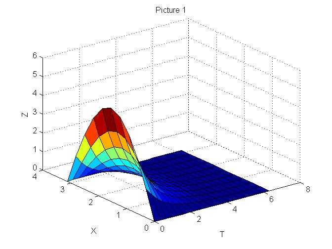
Let consider a linear partial differential equation of the $22$ order in two variables

$$\frac{\partial}{\partial t}\Psi(t,x)=A(t,x)\times\frac{\partial^{2}}{\partial x^{2}}\Psi(t,x)+B(t,x)\times\frac{\partial^{22}}{\partial x^{22}}\Psi(t,x)~{}((t,x)\in[0,2\pi[\times[0,\pi[)$$

with initial condition

$$\Psi(0,x)=\frac{0.015}{2}+5\sin(x),$$

where

$$A(t,x)=\chi_{[0,\pi[\times[0,\pi[}(t,x)+1.55\times\chi_{[\pi,2\pi[\times[0,\pi[}(t,x)$$

and

$$B(t,x)=2\times\chi_{[0,\pi[\times[0,\pi[}(t,x)-2\times\chi_{[\pi,2\pi[\times[0,\pi[}(t,x).$$

The programm in MathLab for a solution of $(3.18)-(3.19)$, has the following form:

$A1=[0,1,0,0,0,0,0,0,0,0,0,0,0,0,0,0,0,0,0,0,0,2];$

$A2=[0,1.55,0,0,0,0,0,0,0,0,0,0,0,0,0,0,0,0,0,0,0,-2];$

$C1=[0,0,0,0,0,0,0,0,0,0,0,0,0,0,0,0,0,0,0,0];$

$D1=[5,0,0,0,0,0,0,0,0,0,0,0,0,0,0,0,0,0,0,0];$

$A10=0;A20=0;C10=0.015;$

for $k=1:20$

$S1(k)=A10;S2(k)=A20;$

for $n=1:10$

$S1(k)=S1(k)+(-1)^{(}n)*A1(2*n)*k^{(}2*n);$

$S2(k)=S2(k)+(-1)^{(}n)*A2(2*n)*k^{(}2*n);$

end

end

for $k=1:20$

$O1(k)=0;$

$O2(k)=0;$

end

for $k=1:20$

for $n=1:10$

$O1(k)=O1(k)+(-1)^{n}*A1(2*n+1)*k^{(}2*n+1);$

$O2(k)=O2(k)+(-1)^{n}*A2(2*n+1)*k^{(}2*n+1);$

end

end

$[T1,X1]=\mbox{meshgrid}(0:(pi/10):pi,0:(pi/10):pi);$

$Z1=0.5*C10*\exp(T1.*A10);$

for $k=1:20$

$Z1=Z1+C1(k)*\exp(T1*S1(k)).*\cos(X1.*k).*\cos(T1*O1(k))+D1(1)*\exp(T1*S1(k)).*\cos(X1.*k).*\sin(T1*O1(k))+$

$D1(k)*\exp(T1*S1(k)).*\sin(X1.*k).*\cos(T1*O1(k))-C1(k)*\exp(T1*S1(k)).*\sin(X1.*k).*\sin(T1*O1(k));$

end

$C20=\exp(pi*(A10-A20))*C10;$

for $k=1:20$

$A(k)=\exp((S1(k)-S2(k))*pi)*(C1(k)*\cos(O1(k)*pi)+D1(k)*\sin(O1(k)*pi));$

$B(k)=\exp((S1(k)-S2(k))*pi)*(D1(k)*\cos(O1(k)*pi)-C1(k)*\sin(O1(k)*pi));$

end

for $k=1:20$

$C2(k)=A(k)*\cos(O2(k)*pi)-B(k)*\sin(O2(k)*pi);$

$D2(k)=B(k)*\cos(O2(k)*pi)+A(k)*\sin(O2(k)*pi);$

end

$[T2,X2]=\mbox{meshgrid}(pi:(pi/10):(2*pi),0:(pi/10):pi);$

$Z2=0.5*C20*exp((T2)*A20);$

for $k=1:20$

$Z2=Z2+C2(k)*\exp(T2*S2(k)).*\cos(X2.*k).*\cos(T2*O2(k))+D2(1)*\exp(T2*S1(k)).*\cos(X2.*k).*\sin(T2*O2(k))+$

$D2(k)*\exp(T2*S2(k)).*\sin(X2.*k).*\cos(T2*O2(k))-C2(k)*\exp(T2*S2(k)).*\sin(X2.*k).*\sin(T2*O2(k));$

end

$\mbox{surf}(T1,X1,Z1)$

hold on

$\mbox{surf}(T2,X2,Z2)$

hold off

 1.: Graphic of the solution of the LPDE-(3.18) with IC-(3.19)).

Example 3.4.

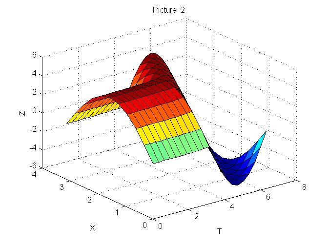
Let consider a linear partial differential equation of the $22$ order in two variables ∂∂tΨ(t,x)=A(t,x)Ψ(t,x)+ B(t,x)×∂2∂x2Ψ(t,x)+C(t,x)×∂3∂x3Ψ(t,x)+

 2.: Graphic of the solution of the LPDE-(3.20) with IC-(3.21)).

D(t,x)×∂22∂x22Ψ(t,x) ((t,x) ∈[0,2π[×[0,π[) with initial condition Ψ(0,x)=0.0152+5sin(x), where A(t,x)=1χ_[0,π[×[0,π[(t,x)+0 ×χ_[π,2π[×[0,π[(t,x), B(t,x)=χ_[0,π[×[0,π[(t,x)+0 ×χ_[π,2π[×[0,π[(t,x), C(t,x)=0×χ_[0,π[×[0,π[(t,x)+1 ×χ_[π,2π[×[0,π[(t,x) and D(t,x)=2×χ_[0,π[×[0,π[(t,x)+2 ×χ_[π,2π[×[0,π[(t,x).

The graphical solution of (3.20)-(3.21) can be obtained by MathLab programm used in Example 3.3 for the following data:

$A1=[0,1,0,0,0,0,0,0,0,0,0,0,0,0,0,0,0,0,0,0,0,2];$

$A2=[0,0,1,0,0,0,0,0,0,0,0,0,0,0,0,0,0,0,0,0,0,2];$

$C1=[0,0,0,0,0,0,0,0,0,0,0,0,0,0,0,0,0,0,0,0];$

$D1=[5,0,0,0,0,0,0,0,0,0,0,0,0,0,0,0,0,0,0,0];$

$A10=1;A20=0;C10=0.015;$

Example 3.5.

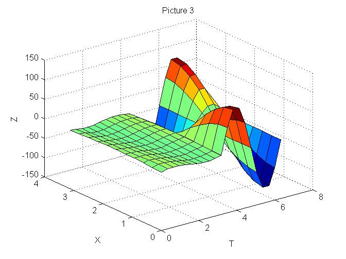
Let consider a linear partial differential equation of the $21$ order in two variables with constant coefficients ∂∂tΨ(t,x)=A(t,x)Ψ(t,x)+ ∂2∂x2Ψ(t,x)+2 ∂21∂x21Ψ(t,x) ((t,x) ∈[0,2π[×[0,π[)

 3.: Graphic of the solution of the LPDE-(3.22) with IC-(3.23)).

with initial condition Ψ(0,x)=0.152+5sin(x), where A(t,x)=1χ_[0,π[×[0,π[(t,x)+0 ×χ_[π,2π[×[0,π[(t,x).

Since 1=1 ×χ_[0,π[×[0,π[(t,x)+1 ×χ_[π,2π[×[0,π[(t,x) and 2=2×χ_[0,π[×[0,π[(t,x)+2 ×χ_[π,2π[×[0,π[(t,x), the graphical solution of (3.22)-(3.23) can be obtained by MathLab programm used in Example 3.3 for the following data:

$A1=[0,1,0,0,0,0,0,0,0,0,0,0,0,0,0,0,0,0,0,0,2,0];$

$A2=[0,1,0,0,0,0,0,0,0,0,0,0,0,0,0,0,0,0,0,0,2,0];$

$C1=[0,0,0,0,0,0,0,0,0,0,0,0,0,0,0,0,0,0,0,0];$

$D1=[5,0,0,0,0,0,0,0,0,0,0,0,0,0,0,0,0,0,0,0];$

$A10=1;A20=0;C10=0.15;$

Example 3.6.

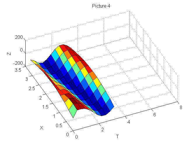
Let consider a linear partial differential equation of the $21$ order in two variables ∂∂tΨ(t,x)=A(t,x)Ψ(t,x)+ B(t,x)×∂2∂x2Ψ(t,x)+100∂3∂x3Ψ(t,x) 2∂21∂x21Ψ(t,x) ((t,x) ∈[0,2π[×[0,π[)

 4.: Graphic of the solution of the LPDE-(3.24) with IC-(3.25)).

with initial condition Ψ(0,x)=0.0152+100sin(x), where A(t,x)=1χ_[0,π[×[0,π[(t,x)+0 χ_[π,2π[×[0,π[(t,x) and B(t,x)=χ_[0,π[×[0,π[(t,x)- χ_[π,2π[×[0,π[(t,x).

The graphical solution of (3.24)-(3.25) can be obtained by MathLab programm used in Example 3.3 for the following data:

$A1=[0,1,100,0,0,0,0,0,0,0,0,0,0,0,0,0,0,0,0,0,2,0];$

$A2=[0,-1,100,0,0,0,0,0,0,0,0,0,0,0,0,0,0,0,0,0,2,0];$

$C1=[0,0,0,0,0,0,0,0,0,0,0,0,0,0,0,0,0,0,0,0];$

$D1=[100,0,0,0,0,0,0,0,0,0,0,0,0,0,0,0,0,0,0,0];$

$A10=1;A20=0;C10=0.15;$

We see that we have no graphic on the region $[\pi,2\pi[\times[0,\pi[$ which hints us that coefficients of the LPDE (3.24)-(3.25) on that region do not satisfy conditions of Theorem 3.2.

Example 3.7.

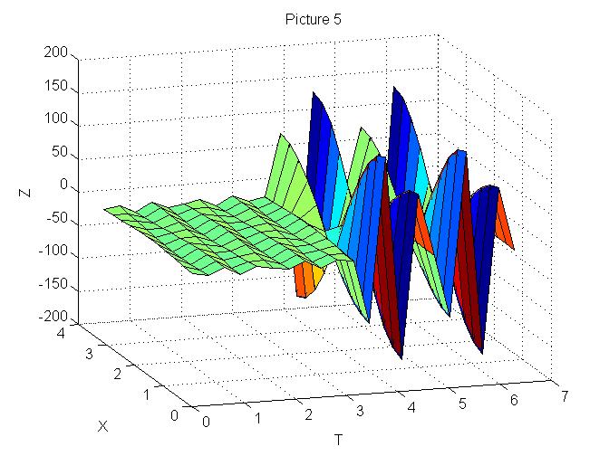
Let consider a linear partial differential equation of the $21$ order in two variables ∂∂tΨ(t,x)=A(x,t)Ψ(t,x)+ 50∂5∂x5Ψ(t,x)+ ∂6∂x6Ψ(t,x) + 2 ∂21∂x21Ψ(t,x) ((t,x) ∈[0,2π[×[0,π[)

 5.: Graphic of the solution of the LPDE-(3.26) with IC-(3.27)).

with initial condition Ψ(0,x)=0.152+5sin(x), where A(t,x)=χ_[0,π[×[0,π[(t,x)+0×χ_[π,2π[×[0,π[(t,x).

The graphical solution of (3.26)-(3.27) can be obtained by MathLab programm used in Example 3.3 for the following data:

$A1=[0,0,0,0,50,1,0,0,0,0,0,0,0,0,0,0,0,0,0,0,2,0];$

$A2=[0,0,0,0,50,1,0,0,0,0,0,0,0,0,0,0,0,0,0,0,2,0];$

$C1=[0,0,0,0,0,0,0,0,0,0,0,0,0,0,0,0,0,0,0,0];$

$D1=[7,0,0,0,0,0,0,0,0,0,0,0,0,0,0,0,0,0,0,0];$

$A10=1;A20=0;C10=0.15;$

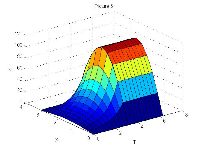
 6.: Graphic of the solution of the LPDE-(3.28) with IC-(3.29)).

Example 3.8.

Let consider a linear partial differential equation of the $22$ order in two variables ∂∂tΨ(t,x)=A(x,t)Ψ(t,x)- ∂∂xΨ(t,x)+2 ∂22∂x22Ψ(t,x) ((t,x) ∈[0,2π[×[0,π[)

with initial condition Ψ(0,x)=0.0152+5sin(x), where A(t,x)=χ_[0,π[×[0,π[(t,x)+0×χ_[π,2π[×[0,π[(t,x).

The graphical solution of (3.28)-(3.29) can be obtained by MathLab programm used in Example 3.3 for the following data:

$A1=[-1,0,0,0,0,0,0,0,0,0,0,0,0,0,0,0,0,0,0,0,0,2];$

$A2=[-1,0,0,0,0,0,0,0,0,0,0,0,0,0,0,0,0,0,0,0,0,2];$

$C1=[0,0,0,0,0,0,0,0,0,0,0,0,0,0,0,0,0,0,0,0];$

$D1=[5,0,0,0,0,0,0,0,0,0,0,0,0,0,0,0,0,0,0,0];$

$A10=1;A20=0;C10=0.015;$

Remark 3.9.

Notice that for each natural number $M>1$, one can easily modify the MathLab program described in Example 3.3 for obtaining the graphical solution of the linear partial differential equation (3.1)-(3.2) whose coefficients $(A_{n}(t,x))_{0\leq n\leq 2M}$ are real-valued simple step functions on $[0,T[\times[-l,l[$ and $f$ is a trigonometric polynomial on $[-l,l[$.

Remark 3.10.

Since each constant $c$ same times is a step function we can use MathLab program described in Example 3.3 for a solution of the linear partial differential equation (2.17)-(2.18) with constant coefficients.

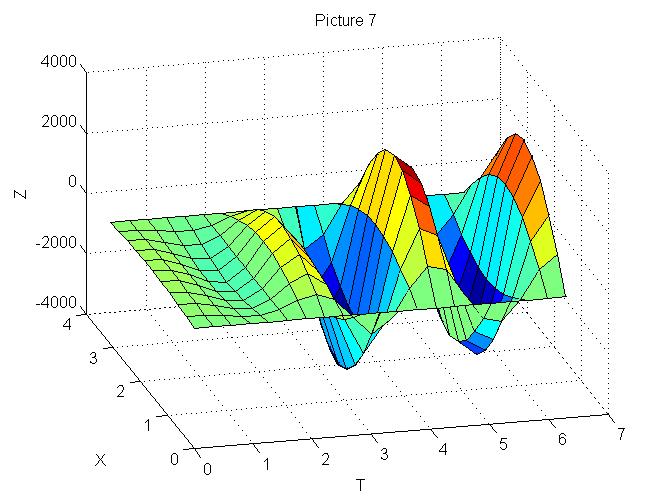
For example, if we consider LPDE ∂∂tΨ(t,x)=-∂∂xΨ(t,x) + ∂3∂x3Ψ(t,x)-∂5∂x5Ψ(t,x)+ ∂7∂x7Ψ(t,x)+2 ∂22∂x22Ψ(t,x) ((t,x) ∈[0,2π[×[0,π[)

 7.: Graphic of the solution of the LPDE-(3.30) with IC-(3.1)).

with initial condition Ψ(0,x)=0.0152+150 sin(x), then for a solution (3.30)-(3.31),in MathLab programm described in Example 3.3 we must enter the following data:

$A1=[-1,0,1,0,-1,0,1,0,0,0,0,0,0,0,0,0,0,0,0,0,0,2];$

$A2=[-1,0,1,0,-1,0,1,0,0,0,0,0,0,0,0,0,0,0,0,0,0,2];$

$C1=[0,0,0,0,0,0,0,0,0,0,0,0,0,0,0,0,0,0,0,0];$

$D1=[150,0,0,0,0,0,0,0,0,0,0,0,0,0,0,0,0,0,0,0];$

$A10=1;A20=0;C10=0.015;$

Remark 3.11.

The approach used for a solution of (3.1)-(3.2) can be used in such a case when coefficients $(A_{n}(t,x))_{0\leq n\leq 2M}$ are rather smooth continuous functions on $[0,T[\times[-l,l[$. If we will approximate $(A_{n}(t,x))_{0\leq n\leq 2M}$ by real-valued simple step functions, then it is natural to wait that under some ”nice restrictions” on $(A_{n}(t,x))_{0\leq n\leq 2M}$ the solutions obtained by Theorem 3.2, will give us a ”good approximation” of the solution of the required linear partial differential equation of the higher order in two variables with corresponding initial conditions.

References

• [1] Linear differential equation, http://en.wikipedia.org/wiki/Linear-differential-equation.
• [2] G.Birkhoff, G. Rota, Ordinary Differential Equations, New York: John Wiley and Sons, Inc., 1978.
• [3] Gantmacher F. R., Theorie des matrices. Tome 111: Theorie generale, Traduit du Russe par Ch. Sarthou. Collection Universitaire de Mathematiques, No. 18. Dunod, Paris (1966).
• [4] J.C. Robinson, An Introduction to Ordinary Differential Equations, Cambridge, UK.: Cambridge University Press, 2004.
• [5] G.Pantsulaia, G.Giorgadze, On some applications of infinite-dimensional cellular matrices, Georg. Inter. J. Sci. Tech., Nova Science Publishers, Volume 3, Issue 1 (2011), 107-129.
• [6] A. Stanoyevitch, Introduction to MATLAB ® with numerical preliminaries, Wiley-Interscience [John Wiley &\& Sons], Hoboken, NJ, 2005. x+331 pp.