Sparse Automatic Differentiation for Complex Networks of Differential-Algebraic Equations Using Abstract Elementary Algebra

Abstract.

Most numerical solvers and libraries nowadays are implemented to use mathematical models created with language-specific built-in data types (e.g. real in Fortran or double in C) and their respective elementary algebra implementations. However, the built-in elementary algebra typically has limited functionality and often restricts the flexibility of mathematical models and the analysis types that can be applied to those models. To overcome this limitation, a number of domain-specific languages such as gPROMS or Modelica with more feature-rich built-in data types have been proposed. In this paper, we argue that if numerical libraries and solvers are designed to use abstract elementary algebra rather than the language-specific built-in algebra, modern mainstream languages can be as effective as any domain-specific language. We illustrate our ideas using the example of sparse Jacobian matrix computation. We implement an automatic differentiation method that takes advantage of sparse system structures and is straightforward to parallelize in a distributed memory setting. Furthermore, we show that the computational cost scales linearly with the size of the system.

1. Introduction

Differential-algebraic equations (DAEs) are ubiquitous in systems engineering problems, especially in design applications [5, 25, 27, 11, 12]. Mathematical models in this area are typically heterogeneous and very sparse. Obtaining the sparse Jacobian for such problems is critical for successful solving or preconditioning strategies.

Additional challenges arise from the need to effectively manage the complexity of system engineering models. The model equations are typically not in a single central place, but assembled from component model equations loaded from multiple dynamic libraries. Furthermore, the component model structure can (and often does) change at runtime. For example, when designing a heat exchanger one may want to keep inlet and outlet temperatures constant at operating conditions and optimize the heat exchanger geometry parameters. In the transient simulations, however, the heat exchanger geometry is fixed and temperatures are system variables. The variable and parameter designation is selected by the designer as needed at runtime. The ability to reuse the same model for different types of analyses is required to reduce the cost of the computation deployment as well as the cost of component model verification and validation.

To address these requirements, domain-specific modeling languages based on symbolic code manipulations such as gPROMS [17] and Modelica [18] have been introduced. Tools built around these languages [6, 26, 15, 20, 16] allow engineers to work in a more interactive design environment where they can make modifications of their models at runtime. These tools go beyond Jacobian generation and perform a number of transformations on the mathematical model, such as causalization, tearing, and index reduction to make subsequent simulations more efficient (see e.g. [3] and references therein). Under the hood, the model encoded in the domain-specific language is processed symbolically and code compatible with the numerical solver is generated and compiled on the fly. Then, such a hard-wired precompiled model is simulated and the result is returned to the user. This approach was pioneered in compiler automatic differentiation tools such as ADIC [2] and OpenAD/F [23].

Symbolic manipulations and compiling automatically generated code on the fly allow one to reuse models coded in a domain-specific language for different types of analyses using different numerical solvers. The downside is that the model needs to be regenerated and recompiled every time the model structure is modified. Scaling up this approach to more complex problems is another challenge as the symbolic preprocessing of model equations may become a bottleneck. In such a framework one needs to support two different parallelization schemes – one for the symbolic manipulations of the model equations and another one for solving these equations numerically. Symbolic transformations are generally nontrivial to parallelize. The more features the domain-specific language offers, the more complex the symbolic processing algorithms become and so does their parallel implementation. At the time of this writing, we are not aware of distributed memory parallel schemes for the symbolic processing of mathematical equations.

Modern object-oriented languages, such as C++, which support operator overloading, template specialization, type traits, and other advanced features allow one to create numerical models that can be reconfigured at runtime. In this paper we argue that the same functionality provided by symbolic preprocessing of the model equations can be implemented by creating custom data types and appropriate libraries in mainstream object-oriented languages. Recently, solver frameworks that use abstract data types were proposed [1]. Those frameworks do not require specific data types to be used, but only specify elementary algebra that the data types have to support. By designing models and solvers to use abstract data types, one can reuse the same models and solvers for multiple analysis types such as forward simulations, optimization, sensitivity analysis, or embedded uncertainty quantification [4]. Switching between these may be accomplished simply by changing (or reconfiguration of) the data type. Furthermore, abstract data types can be used to compute automatically the system connectivity graph which could then be utilized, for instance, to partition the system into smaller subsystems, perform index reduction for differential-algebraic equations, implement tearing algorithms, and many other calculations.

We illustrate this abstract elementary algebra approach by developing a method for sparse automatic Jacobian generation, which is superior to other available methods when applied to systems engineering problems. We show that our method allows for model reconfiguration at runtime and overall better code reuse in scientific applications. Moreover, we show that our approach enables the automatic generation of the dependency graph of a system. The method is straightforward to parallelize in a distributed memory environment.

A similar approach is used in Sacado [19], an automatic differentiation package which is part of the Trilinos library [9]. However, Sacado does not support sparse derivatives – it allocates memory for derivatives with respect to all system variables. For many partial differential equation (PDE) models this is not a significant limitation since the sparsity pattern typically consists of locally dense cells and dense derivatives can be computed for each cell separately. Automatic differentiation also can be incorporated directly in the mesh generation (e.g. as in [22]), therefore using sparsity information from the mesh itself. On the other hand, components in system engineering applications are often large with locally sparse structures that can be exploited by using sparse automatic differentiation.

The automatic differentiation library ADOL-C [24] provides sparse capability and has drivers for computing Jacobian and Hessian matrices. However, ADOL-C does not define abstract elementary algebra, but uses operator overloading only locally to compute derivatives. Such approach requires ADOL-C specific code in the model, and is not easily extensible. Furthermore, ADOL-C does not support distributed memory parallelization.

The paper is organized as follows: In Section 2 we provide the mathematical formulation of the elementary algebra we use for sparse automatic differentiation. We describe the prototype C++ implementation in Section 3. Preliminary benchmarking results showing linear scaling of the computational cost are presented in Section 4. Future research directions are discussed in Section 5.

2. Mathematical Formulation of Sparse Automatic Differentiation

2.1. Problem Description

In addition to the system of nonlinear equations or differential-algebraic equations, given by

$$f(x;p)=0\quad\text{or}\quad F(t,x,\dot{x};p)=0,$$ (1)

respectively, most numerical libraries for the solution and optimization of such systems require the user to provide also the Jacobian and the sparsity pattern of the system. Here, $x$ is the vector of variables and $p$ the vector of parameters. The Jacobian $J$ is then defined as the matrix

$$J=\frac{\partial f}{\partial x}\quad\text{or}\quad J=\alpha\frac{\partial F}{\partial\dot{x}}+\frac{\partial F}{\partial x},$$ (2)

where the parameter $\alpha$ is related to the numerical integration scheme used for the simulation and provided by the solver. There are several different ways to compute the Jacobian:

• Compute and implement analytical Jacobian manually. While this will lead to the fastest numerical computations, it is often not feasible or extremely cumbersome to compute Jacobians manually for large systems.

• Compute Jacobian numerically. The derivatives can be computed using finite difference approximations. This approach is relatively easy to implement, but it is in general neither accurate nor efficient.

• Use compiler automatic differentiation. This approach requires equation syntax parsing capabilities. For large systems, parsing the equations can be quite time consuming. Parallelizing these methods could be quite challenging, as well.

• Use operator overloading automatic differentiation. In this approach, all derivatives are computed automatically at the same time when the model equations are evaluated. This approach requires minimal involvement from the component model developer.

Another requirement is often to be able to reuse model equations in cases where some of the parameters $p_{i}$ are set as variables and some of the variables $x_{i}$ are “fixed” to constant values. Each of those cases would require different Jacobians. This complicates implementing the first and third approach for such systems significantly.

For most engineering problems, the governing equations are sparsely coupled. Thus, only a small fraction of the entries of the Jacobian will be nonzero. There are a number of different algorithms for solving linear systems that take advantage of the system sparsity to speed up computations [13, 7]. To use those algorithms, however, one also needs to find the sparsity pattern.

Example 2.1.

Assume we are trying to find a steady state solution for a Lorenz system [14]. The residual equations (1) can be written as

$$\begin{split}\sigma(y-x)&=0,\\ x(\rho-z)-y&=0,\\ xy-\beta z&=0,\end{split}$$ (3)

where $x$, $y$, and $z$ are variables and $\sigma$, $\rho$, and $\beta$ are constant parameters. The Jacobian (2) is then given by

$$J=\begin{bmatrix}-\sigma&\sigma&0\\ \rho-z&-1&-x\\ y&x&-\beta\end{bmatrix}.$$ (4)

Here, $J_{13}\equiv 0$, while all the other entries have nonzero values, generally. The sparsity pattern for the Lorenz system is then

$$\begin{bmatrix}\bullet&\bullet&\\ \bullet&\bullet&\bullet\\ \bullet&\bullet&\bullet\end{bmatrix}.$$ (5)

This tells the solver it does not need to allocate memory for $J_{13}$ and perform computations with it.  $\triangle$

Developing an efficient way for computing the sparsity pattern of the Jacobian is the key enabling technology for solving large-scale nonlinear systems, ordinary differential equations, differential-algebraic equations, and optimization problems. Since all of the information required to compute the Jacobian is contained within the model equations, the computation of the Jacobian and its sparsity pattern can be fully automated.

2.2. Automatic Structure Analysis

For better clarity, let us first discuss the sparsity pattern generation alone. The sparsity pattern is required by the numerical solver at the initialization stage to allocate objects required for sparse linear algebra algorithms. During computations, the sparsity pattern (i.e. connectivity structure) is used by the linear solver to identify structurally nonzero elements of the Jacobian that enter the computation.

The system connectivity information can be used for a number of other analyses such as index reduction for differential-algebraic equations (DAEs), partitioning, model causalization, tearing, numerical diagnostics, and many others. These are, however, beyond the scope of this paper and will be only briefly described in Subsection 2.4.

The approach we propose is to compute the dependencies of the residual equations on the fly along with the residual values. To do that, we define a mathematical object $\mathcal{Y}$ which is a set containing a real number $y$ and set $\mathbb{D}$, which contains integer labels of all dependencies of $y$. Labels are independent variable identifiers; typically, they are offset values in the solution vector as returned by the solver. We denote this object as

$$\mathcal{Y}=\{y,\mathbb{D}_{y}\}.$$ (6)

For any independent variable $x$, the corresponding dependency tracking object is

$$\mathcal{X}=\{x,\{n_{x}\}\},$$ (7)

that is, each independent variable has only trivial self-dependency. Algebraic operations on $\mathbb{Y}$, the set of all $\mathcal{Y}$, are defined as follows:

• For any $C\in\mathbb{R}$ and $\mathcal{Y}\in\mathbb{Y}$ and algebraic operation $*$, it is

  $$C*\mathcal{Y}=\{C*y,\,\mathbb{D}_{y}\}.$$ (8)

• For any two $\mathcal{Y},\,\mathcal{Z}\in\mathbb{Y}$ and mathematical operation $*$, it is

  $$\mathcal{Y}*\mathcal{Z}=\{y*z,\,\mathbb{D}_{y}\cup\mathbb{D}_{z}\}.$$ (9)

• For any function $h(y)$ defined on $\mathbb{R}$, there is a corresponding function $h(\mathcal{Y})$ defined on $\mathbb{Y}$ such that

  $$h(\mathcal{Y})=\{h(y),\,\mathbb{D}_{y}\},$$ (10)

  where $\mathbb{D}_{y}$ is the set of dependencies of $\mathcal{Y}$.

Comparisons between elements of $\mathbb{Y}$ are performed with respect to values only, disregarding dependencies. For example:

$$\mathcal{Y}_{1}>\mathcal{Y}_{2}\,\,\Leftrightarrow\,\,y_{1}>y_{2}.$$ (11)

If we define residual equations on $\mathbb{Y}$, rather than $\mathbb{R}$, the residual computation will give us both, the residual value and the sparsity pattern.

Example 2.2.

Let us consider again the Lorenz system introduced in Example 2.1. The first residual is computed as

$$\begin{split}\mathcal{F}_{1}&=\sigma\left(\{x,\{n_{x}\}\}-\{y,\{n_{y}\}\}\right)\\ &=\sigma\{x-y,\{n_{x}\}\cup\{n_{y}\}\}\\ &=\{\sigma(x-y),\{n_{x},n_{y}\}\},\end{split}$$ (12)

and similarly we get

$$\mathcal{F}_{2} =\{x(\rho-z)-y,\{n_{x},n_{y},n_{z}\}\},$$ (13)

$$\mathcal{F}_{3} =\{xy-\beta z,\{n_{x},n_{y},n_{z}\}\}.$$ (14)

From the dependencies in (12–14), one can obtain the sparsity pattern (5) by setting $n_{x}=1$, $n_{y}=2$, and $n_{z}=3$. Note that this approach for obtaining the sparsity pattern is independent of how equations are written. If we, for example, write the third residual in (3) as

$$f_{3}=u-\beta z,$$ (15)

where $u=xy$, then the residual evaluation using dependency tracking variables gives us

$$\begin{split}\mathcal{F}_{3}&=\{u,\mathbb{D}_{u}\}-\beta\{z,\{n_{z}\}\}\\ &=\{xy,\{n_{x}\}\cup\{n_{y}\}\}-\{\beta z,\{n_{z}\}\}\\ &=\{xy-\beta z,\,\{n_{x},n_{y}\}\cup\{n_{z}\}\}\\ &=\{xy-\beta z,\,\{n_{x},n_{y},n_{z}\}\},\end{split}$$ (16)

which is the same as (14).  $\triangle$

This property is particularly convenient when coding residual equations because it allows reordering computations and using as many intermediate dependent variables as necessary. Note that all derivatives in the equations are uniquely defined in terms of derivatives with respect to independent variables, only.

2.3. Automatic Differentiation

To perform sparse automatic differentiation we make a small extension to the object we used for the sparsity pattern computation. We define $\tilde{\mathbb{Y}}$ as a set of all

$$\tilde{\mathcal{Y}}=\{y,\,\{(n,\partial_{n}y):n\in\mathbb{D}_{y}\}\},$$ (17)

where $y$ and $\mathbb{D}_{y}$ are the same as in (6). Essentially, we mapped to each dependency the value of the partial derivative with respect to that dependency. For independent variables

$$\tilde{\mathcal{X}}=\{x,\,\{(n_{x},1)\}\}.$$ (18)

Algebraic operations on $\tilde{\mathbb{Y}}$ are defined in a similar fashion as in the dependency tracking case:

• For any $C\in\mathbb{R}$, $\tilde{\mathcal{Y}}\in\tilde{\mathbb{Y}}$ and algebraic operation $*$ defined on $\tilde{\mathbb{Y}}$, it is

  $$C*\tilde{\mathcal{Y}}=\{C*y,\,\{(n,\partial_{n}(C*y)):n\in\mathbb{D}_{y}\}\}.$$ (19)

• For any two $\tilde{\mathcal{Y}},\tilde{\mathcal{Z}}\in\tilde{\mathbb{Y}}$ and algebraic operation $*$ defined on $\tilde{\mathbb{Y}}$, it is

  $$\tilde{\mathcal{Y}}*\tilde{\mathcal{Z}}=\{y*z,\,\{(n,\partial_{n}(y*z)):n\in\mathbb{D}_{y}\cup\mathbb{D}_{z}\}\}.$$ (20)

• For any function $h(x)$ defined on $\mathbb{R}$, there is a corresponding function $h(\tilde{\mathcal{Y}})$ defined on $\tilde{\mathbb{Y}}$ such that

  $$h(\tilde{\mathcal{Y}})=\{h(y),\,\{(n,h^{\prime}(y)\partial_{n}y):n\in\mathbb{D}_{y}\}\},$$ (21)

  where $\mathbb{D}_{y}$ is the set of dependencies of $\tilde{\mathcal{Y}}$.

Comparisons between elements of $\tilde{\mathcal{Y}}$ are defined in the same way as for the dependency tracking data type.

Example 2.3.

Let us compute the Jacobian for residual (15). Using the automatic differentiation data type defined in (17), and the algebra defined for it, this computation is carried out as

$$\begin{split}\mathcal{F}_{3}&=\{u,\{(n_{x},\partial_{x}u),(n_{y},\partial_{y}u)\}\}-\beta\{z,\{(n_{z},1)\}\}\\ &=\{xy,\{(n_{x},y),(n_{y},x)\}\}-\{\beta z,\{(n_{z},\beta)\}\}\\ &=\{xy-\beta z,\,\{(n_{x},y),(n_{y},x),(n_{z},-\beta)\}\}.\end{split}$$

The derivatives in $\mathcal{F}_{3}$ make up the third row of the Jacobian (4), when $n_{x}=1$, $n_{y}=2$, and $n_{z}=3$.  $\triangle$

2.4. Further Applications

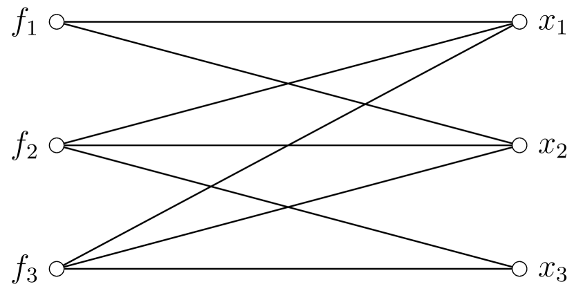
Analogously, the structure of a given system can be represented as a bipartite graph, where the bipartite sets of vertices are the equations and variables, respectively. Equation $f_{i}$ is then by definition connected to variable $x_{j}$ if and only if $J_{ij}\not\equiv 0$. The dependency graph of the Lorenz system (3) is shown in Figure 1a. These dependency graphs are typically used for symbolic transformations such as causalization and tearing of model equations. The causalization selects the order in which equations are solved, so that system can be solved gradually, piece by piece. Tearing is typically used in conjunction with causalization to break dependency loops. These methods are described in detail in [3], for example. With our data type, the dependency graph is automatically generated during the model evaluation and these methods can be implemented without source code transformation tools.

a)

b)

Figure 1. a) Dependency graph of the Lorenz system. b) Partitioning of two coupled Lorenz systems using the dependency graph. Only the edge marked in red needs to be shared by the two cores.

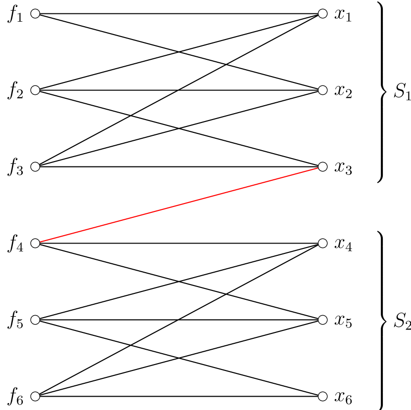
The dependency graph could also be used to decompose a high-dimensional system into smaller subsystems. With the aid of graph partitioning tools, it would be possible to break the system into smaller clusters that are strongly connected internally, but only weakly connected to the other clusters. In this way, assigning different clusters or subsystems to different processing cores, the communication between cores – which is often a bottleneck during the parallel simulation of such systems – could be minimized without domain knowledge simply by using a data type that tracks the dependencies. An illustration of this approach is shown in Figure 1b, where two coupled Lorenz systems are split into subsystems $S_{1}$ and $S_{2}$. Here, only variable $x_{3}$ is required by both subsystems and needs to be shared by the two cores if the system is solved in parallel. Note that subsystem $S_{1}$ can be evaluated independently whereas $S_{2}$ depends on $S_{1}$. This can also be regarded as a block causalization of the system.

3. Prototype Implementation

Dependency tracking objects like (6) or (17) can be seamlessly implemented in any programming language that supports operator overloading. We created a preliminary implementation in C++ mainly for prototyping and testing purposes. Here, we outline the details of this implementation.

We create a class Variable that stores the double precision value and the dependency map related to that value. The class overloads all operators defined for the double data type. The prototype implementation is structured like this:

⬇

class Variable

{

public:

Variable();

explicit Variable(double value);

Variable(double value, size_t variableID);

Variable(const Variable& v);

$\sim$Variable();

// =

Variable& operator=(const double& rhs);

Variable& operator=(const Variable& rhs);

// +=

Variable& operator+=(const double& rhs);

Variable& operator+=(const Variable& rhs);

// *=

Variable& operator*=(const double& rhs);

Variable& operator*=(const Variable& rhs);

// ...

typedef std::map<size_t, double> DependencyMap;

private:

double value_;

size_t variableID_;

bool isFixed_;

mutable DependencyMap* dependencies_;

};

This class has several constructors. The constructor that creates Variable from double data type is made explicit to prevent a possible loss of derivatives in accidental implicit data conversions. In addition to the value and the identifier of the variable, the object has a boolean flag isFixed_. This flag is used when the designation of the object needs to change from a variable to a constant parameter. The dependency map in this implementation is just a standard map between the variable identifiers and the values of the derivatives with respect to those variables. Only independent (state) variables have assigned identifiers. The identifiers typically correspond to global vector indices. Dependent or temporary variables would obtain their dependency map directly or indirectly from state variables. For example $x$, $y$, and $z$ in equation (15) would have identifiers set to $1$, $2$, and $3$, respectively, but $u$ would not have an identifier.

All arithmetic operators are overloaded for Variable data type to implement (20) and combinations of Variable and double types to implement (19). Arithmetic operators are implemented in terms of compound assignment operators. For example, here is how *= operator overloading is implemented for the Variable class:

⬇

Variable& Variable::operator*=(const Variable& rhs)

{

// derivation by parts of @ *this

scaleDependencies(rhs.value_);

// compute partial derivatives of rhs and add them to *this

for(auto& p : *(rhs.dependencies_))

(*dependencies_)[p->first] += (p->second * value_);

// compute value of *this

value_ *= rhs.value_;

return *this;

}

Here, we compute the derivative $(lhs\cdot rhs)^{\prime}=(lhs)^{\prime}\cdot rhs+lhs\cdot(rhs)^{\prime}$, where $lhs$ is pointed to by this. The derivatives of $lhs$ are first scaled by the value of $rhs$ to obtain the first term in the expression for the derivative of the product. Then each $rhs$ derivative is multiplied by the value of $lhs$ and added to corresponding derivatives of $lhs$. If the corresponding derivative of $lhs$ does not exist, a new entry is added to the dependency map. The value is computed at the end, because it is used in the derivative of the product expression.

The multiplication operator is then implemented as a non-member operator

⬇

const Variable operator*(const Variable& lhs, const Variable& rhs)

{

return Variable(lhs) *= rhs;

}

The copy constructor with lhs as the argument is used to create the variable to be returned and then the *= operator is used to multiply that variable by rhs.

In addition to overloading operators, all mathematical functions from the standard C++ library operating on double data type have to be overloaded, as well. Take for example the sine function whose derivative is $(\sin x)^{\prime}=\cos x\cdot x^{\prime}$:

⬇

namespace std

{

inline Variable sin(const Variable& x)

{

double val = sin(x.getValue());

double der = sin_derivative(x.getValue());

Variable res(x); // copy derivatives of x

res.setValue(val); // set function value f(x)

res.scaleDependencies(der); // compute derivatives of f(x)

return res;

}

}

In the namespace std we define an inline function that takes a Variable data type as the input. We use the copy constructor to retain all derivatives of $x$, and then we multiply them by $\cos x$ per chain rule. The value of the sine is computed using the sine function from the standard C++ library. The function that computes the derivative of the sine is defined in the same namespace as the Variable type:

⬇

inline double sin_derivative(double x)

{

return std::cos(x);

}

The same approach is used for other functions.

Example 3.1.

A simple use of the Variable class is shown in the following code:

⬇

template <typename T>

void residualFunction(vector<T>& f,

const vector<T>& x,

const vector<T>& p)

{

const T y = x[0]*x[1];

f[0] = p[0]*(x[1] - x[0]); // sigma*(y - x)

f[1] = x[0]*(p[1] - x[2]) - x[1]; // x*(rho - z) - y

f[2] = y - p[2]*x[2]; // x*y - beta*z

}

int main()

{

const size_t n = 3;

vector<Variable> x(n), p(n), f(n);

// initialize independent variables

x[0] = 8.0; x[1] = 20.0; x[2] = 2.0/3.0;

// set constant parameter values

p[0] = 10.0; p[1] = 8.0/3.0; p[2] = 28.0;

// decide x, y, and z are variables...

for (size_t i = 0; i < n; ++i)

x[i].setVariableNumber(i);

// ...and sigma, rho, and beta are constant parameters

for (size_t i = 0; i < n; ++i)

p[i].setFixed(true);

residualFunction(f, x, p);

printIncidenceMatrix(f);

printJacobian(f);

}

The function residualFunction computes the residual for the steady state solution of the Lorenz system. The dependent variable y is not really needed in this example other than to illustrate how the derivative calculation is propagated through variables. It is important to note that the Lorenz model in this implementation does not depend on a specific data type. Furthermore, the model does not assume what are independent variables and what are system parameters. This is determined outside the model. In this example, elements of the vector x are set to be independent variables and elements of the vector p constant parameters in the main function. This is consistent with the problem defined in (3) where we look for a steady state solution given parameters $\sigma$, $\rho$ and $\beta$. One residual evaluation with the Variable data type also computes the sparsity pattern and the Jacobian. The function printIncidenceMatrix outputs the sparsity pattern:

⬇

A = [1 1 0;

1 1 1;

1 1 1];

The function printJacobian outputs:

⬇

J = [-10 10 0;

2 -1 -8;

20 8 -28];  $\triangle$

Postprocessing of this output may help, for instance, detect (structurally) singular or ill-conditioned Jacobians. For simplicity, we omit the implementation of the two output functions. Note that in this example the parameters p could be declared as double instead of Variable, thus getting rid of a small overhead when calling p. In that case, however, we would need to modify residualFunction code if we wanted to change parameter and variable designation as in the next example.

Example 3.2.

The Variable data type allows us to change parameter and variable designations at runtime, so we can designate elements of the vector p as system variables and elements of the vector x as constant system parameters. All one has to do is to set:

⬇

// decide x, y, and z are constant parameters...

for (size_t i = 0; i < n; ++i)

x[i].setFixed(true);

// ...and sigma, rho, and beta are variables

for (size_t i = 0; i < n; ++i)

p[i].setVariableNumber(i);

In this problem we look for parameters $\sigma$, $\rho$, and $\beta$ such that a fixed point solution of (3) is at $x=8$, $y=20$, and $z=2/3$. The sparsity pattern and Jacobian of the system in that case are obtained as

⬇

A = [1 0 0;

0 1 0;

0 0 1];

and

⬇

J = [12 0 0;

0 8 0;

0 0 -0.667];

respectively. This change can be made at runtime without the need to recompile the system model. Any other selection of system parameters and variables can be made in the same way. The vectors x and p are used merely to denote nominal system variables and parameters.  $\triangle$

Typically, one would run the residual evaluation with dependency tracking during the solver initialization phase to get the sparsity pattern, and then run the residual evaluation with derivative calculation every time the Jacobian is required during solver iterations. Note that the residual vector in this case is in fact an implementation of a compressed row sparse matrix. The only difference is that each row, in addition to matrix elements, also holds a corresponding residual vector element.

4. Preliminary Benchmarking Results

Our approach provides model developers with an intuitive interface, simplifies porting of legacy codes, allows for model equations to be modified at runtime and is straightforward to parallelize. The trade-off is that allocating variables in local scope is expensive and adds significant new overhead to the computation. For our approach to be feasible, the overhead has to be manageable and scale well with the size of the system. To provide a preliminary assessment of how the computational cost scales with the size of the model (i.e. number of equations), we perform several numerical experiments. For the purpose of this assessment, we treat all variables (including residuals) as local scope variables and reallocate derivatives each time they are computed.

Figure 2. Benchmarking test case: A simple electrical grid model.

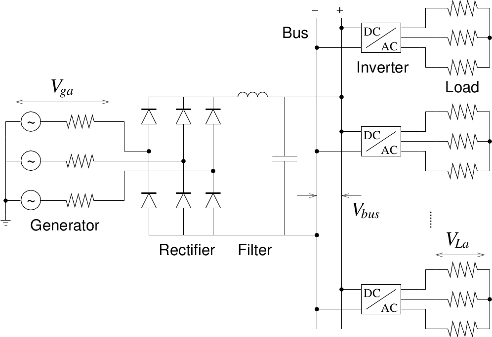
As a benchmark problem, we select a simple microgrid model as shown in Figure 2. A single alternating current (AC) generator is connected to a rectifier that converts power to direct current (DC) and supplies it to a DC bus. Several passive AC loads are connected to the DC bus, each through a separate inverter that converts DC power from the bus to 60$\,\mathrm{Hz}$ AC power required by the load. The size of this system can be easily scaled up by simply adding more loads to the bus. The system parameters are set so that the simulation results are “self-validating” – the voltage at each load is the same as the voltage produced by the generator: 100$\,\mathrm{V}$, 60$\,\mathrm{Hz}$ sinusoidal. A more detailed description of the test case is given in Appendix A.

The electrical grid model is cast in form of differential-algebraic equations. We simulate the first 0.1$\,\mathrm{s}$ of the grid operation using the Rythmos package from the Trilinos library. We use an implicit variable-order variable-stepsize backward differentiation method to solve the equations [10]. The solutions of the resulting systems of nonlinear equations are obtained using a sparse direct method. The method requires the residual equations and the Jacobian of the system to be provided. We measure the overall computation time and model evaluation time. In our case, a model evaluation is a residual evaluation using the Variable data type. The Jacobian is evaluated automatically together with the residual at each model evaluation call per design of the Variable class.

The unknown variables $x$ in our case are typically node voltages. An example of the Jacobian sparsity pattern for the benchmarking test case is shown in Figure 3.

Figure 3. Sparsity pattern for the grid model with 30 loads. Only $1.8\,\%$ of Jacobian elements are structurally nonzero.

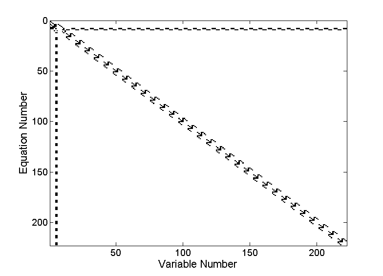
In the serial case, we ran simulations for grids with 100–600 loads. For these simulations it takes roughly 8,000 integrator steps and 50,000–60,000 function evaluations to complete regardless of the size of the system. We find that the average computational time per call grows linearly with the size of the system as shown in Figure 4. Data points for the computational cost of the function evaluation fit particularly well to the linear model.

Figure 4. Wall time for the overall computation and the model evaluation only.

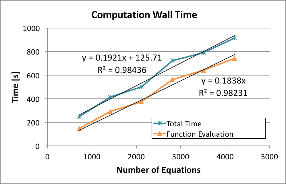
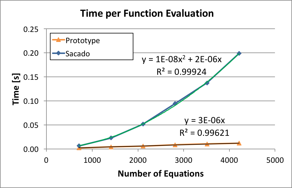
We compare the average cost of the function evaluation for our sparse automatic differentiation prototype with dense automatic differentiation using the Sacado package from the Trilinos library. The prototype uses the class map from the standard C++ library ($O(\log n)$ cost), whereas Sacado uses a dense vector ($O(1)$ cost) to store and access derivatives. We use our method to compute sparsity pattern information and provide it to Sacado, so that only structurally nonzero derivatives are computed. For systems of this size, it was expected that the dense algorithm would outperform the sparse automatic differentiation. Both algorithms evaluate the same derivatives and the dense approach has faster access to derivatives. The only downside of the dense approach is that it has to allocate larger chunks of memory to store derivatives. Yet, our results suggest that memory management alone may cause the computational cost to grow quadratically with the size of the system when using dense automatic differentiation (Figure 5).

Figure 5. Function evaluation cost when using sparse and dense automatic differentiation.

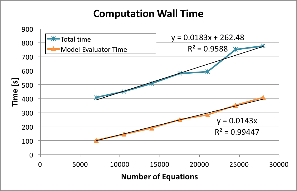
Parallelizing simulations that use sparse automatic differentiation to compute the Jacobian is fairly straightforward in the MPI framework when using our approach. For testing purposes, we implemented a simple parallelization scheme where the generator and the rectifier are simulated on one node and the simulations of inverters and loads are evenly distributed over the remaining nodes. We show here results of an MPI simulation on 16 CPU cores (4 nodes). The number of loads in the system was varied from 1,000–4,000 (roughly 10,000–30,000 equations). The results show again linear scaling as the size of the system increases as shown in Figure 6. Sacado eventually uses up all the memory on the compute node in this case and simulation crashes.

Figure 6. Computational time per call for integration step and function evaluation.

5. Conclusion

Our analysis and benchmarking results suggest that using the proposed abstract elementary algebra approach for sparse automatic differentiation is a promising direction. The linear scaling of the computational costs and the ease of parallelization indicate that this approach is particularly suitable for massively parallel computations.

The prototype implementation leaves room for code optimization. The residual vector implemented in terms of the Variable data type is de facto a compressed row sparse Jacobian with the extension that each row is associated with the corresponding residual value. At this time we have not implemented an option to switch off Jacobian computation when the solver does not need it. Intermediate variables, such as $u$ in (15), can be understood as sparse matrix rows, as well. However, they are not part of the Jacobian, they are used just to complete the chain rule. Typically, intermediate variables are used by system modelers for convenience to write model equations in a more compact form. In the current implementation, derivatives of residual functions are reallocated at every function evaluation based on the dependency tracking mechanism. Since this information does not change during solver iterations, the dependency structure of the system could be precomputed once and then reused at subsequent solver iterations. This could be done easily for residual vectors, which are typically passed by reference to models. Intermediate variables are typically local variables used by the modeler to simplify the equations, so they may have to be reallocated at every iteration anyway. The code optimization and more thorough performance testing will be done in a subsequent work.

When simulating our test cases, we had to copy the residual values from the vector of variables to the Epetra vector and the Jacobian derivatives to a compressed-row sparse matrix provided by Epetra, per requirements of the Rythmos solver. This added a small additional overhead to the computation. The full power of the proposed approach could be demonstrated with numerical solvers that do not require specific data formats, but instead provide abstract interfaces to all linear and elementary algebra operations. While such solvers are still not part of the mainstream, a lot of activities have been done in that direction as for example in Tpetra project [1].

Using abstract elementary algebra has potential applications way beyond automatic differentiation. As we have shown in this paper, it could be used for reconfiguring models at runtime; constant parameters could be changed into variables and vice versa. Abstract data types also could be used for diagnostics, for example to identify structurally singular Jacobians. Furthermore, this approach could be used for preprocessing model equations for index reduction of differential-algebraic equations or tearing algorithms for system decomposition.

Abstract elementary algebra can also help reuse existing code. The same model code can be reused for local sensitivity analysis or embedded uncertainty quantification, simply by using different template parameters. The same holds true for solvers that provide abstract interfaces for elementary algebra. More reuse streamlines code verification and improves development efficiency, which are critical for any large scale computation. All of these will be pursued in subsequent work.

Appendix A Test Case Description

Electrical grids are a common motif in power systems. An example of such a grid is shown in Figure 2. Since mathematical modeling methods for power systems are not commonly known outside the electrical engineering community, we provide here a brief overview of the governing equations used in our test case. For a detailed description of the component models, we refer the reader to, for example, [8] and references therein. The equations are derived and the system is composed using the modified nodal analysis approach [21].

We assume that the generator shown on the left side in Figure 2 is an ideal 3-phase generator with residual equations for the generator terminals $a$, $b$, and $c$ given by:

$$0 =v_{ga}-V_{0}\sin(\omega t),$$ (22)

$$0 =v_{gb}-V_{0}\sin(\omega t+2\pi/3),$$ (23)

$$0 =v_{gc}-V_{0}\sin(\omega t+4\pi/3).$$ (24)

Figure 7. Schematic of the rectifier model.

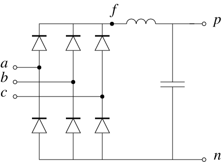
The generator is connected to a rectifier, which converts the 3-phase AC power to DC power. Rectifier and filter schematics are shown in Figure 7. Kirchhoff’s current law for the rectifier can be cast in terms of residual equations as

$$0 =i_{ga}-I_{D}(v_{ga}-v_{f})+I_{D}(v_{n}-v_{ga}),$$ (25)

$$0 =i_{gb}-I_{D}(v_{gb}-v_{f})+I_{D}(v_{n}-v_{gb}),$$ (26)

$$0 =i_{gc}-I_{D}(v_{gc}-v_{f})+I_{D}(v_{n}-v_{gc}).$$ (27)

Here, $i_{ga}$, $i_{gb}$, and $i_{gc}$ are generator phase currents entering the rectifier nodes $a$, $b$, and $c$; $v_{f}$ is the voltage at node $f$ (rectifier’s positive terminal, connected to the filter) and $v_{n}$ is the node voltage at rectifier’s negative terminal.

The current through diodes $I_{D}(v)$ in the rectifier is modeled as

$$I_{D}(v)=I_{s}\left[\exp\left(\frac{v}{nkT}\right)-1\right].$$

In our simulations, we chose the temperature $T=300\,$K, ideality factor $n=2$, and saturation current to be $I_{s}=18.8\,$nA. Boltzmann constant $k\approx 1.38\times 10^{-23}$ J/K. The voltage $v$ in the diode current function is the difference between node voltages at the anode and cathode terminals of the diode.

The residual equations for the filter can be written as

$$0 =I_{D}(v_{ga}-v_{f})+I_{D}(v_{gb}-v_{f})+I_{D}(v_{gc}-v_{f})-i_{L},$$ (28)

$$0 =\phi_{L}-Li_{L},$$ (29)

$$0 =\dot{\phi}_{L}-(v_{f}-v_{p}),$$ (30)

$$0 =q_{C}-C(v_{p}-v_{n}),$$ (31)

where $i_{L}$ and $\phi_{L}$ are inductor’s current and flux, respectively, $L$ is the inductance, $q_{C}$ is charge on the capacitor, $C$ is the capacitance, and $v_{p}$ is the voltage at the positive terminal of the DC bus.

Kirchhoff’s current law gives the following equations for the DC bus (Figure 2):

$$\begin{split}0={}&-\dot{q}_{C}+i_{L}\\ &+\sum_{k}G_{k}\left(d^{(k)}_{a}(t)v^{(k)}_{a}+d^{(k)}_{b}(t)v^{(k)}_{b}+d^{(k)}_{c}(t)v^{(k)}_{c}\right),\end{split}$$ (32)

$$\begin{split}0={}&I_{D}(v_{n}-v_{ga})+I_{D}(v_{n}-v_{gb})+I_{D}(v_{n}-v_{gc})\\ &+\sum_{k}\left(i^{(k)}_{a}+i^{(k)}_{b}+i^{(k)}_{c}\right),\end{split}$$ (33)

where $v^{(k)}_{\alpha}$ and $i^{(k)}_{\alpha}$ are $\alpha$-phase of the voltage across and current through the load $k$ ($\alpha=a,b,c$). The functions $d^{(k)}_{\alpha}(t)$ are inverter modulation signals that describe 3-phase AC waveforms at the inverter outlet. We choose the modulation signals to be the same for all inverters and produce the sinusoidal output:

$$d^{(k)}_{a}(t) =m\sin(\omega t),$$

$$d^{(k)}_{b}(t) =m\sin(\omega t+2\pi/3),$$

$$d^{(k)}_{c}(t) =m\sin(\omega t+4\pi/3).$$

Here, we set $\omega$ to be the same as the frequency of the generator. Furthermore, we set

$$m=\frac{2\pi}{3\sqrt{3}},$$

so that the voltage amplitude at each load is the same as the generator voltage amplitude. This choice was made merely for model verification convenience (again, interested readers are referred to [8] for more details).

Figure 8. Schematic of the inverter model with averaged pulse width modulation.

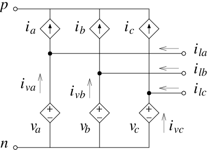
The inverter model we used is an averaged model without details of pulse width modulation. The equivalent circuit model of such an inverter model is shown in Figure 8. The model consists of three ideal current-controlled current sources and three ideal voltage-controlled voltage sources (one for each phase). The current sources are controlled by the load currents as

$$i_{\alpha}=d_{\alpha}(t)i_{l\alpha},\quad\alpha=a,b,c,$$

where $i_{l\alpha}$ is the load current (Figure 8). Voltage sources are controlled by the DC bus voltage as

$$v_{\alpha}=\frac{1}{2}d^{(k)}_{\alpha}(t)(v_{p}-v_{n}),\quad\alpha=a,b,c.$$

Here, $v_{p}$ and $v_{n}$ are the node voltages on the positive and negative terminals of the DC bus, respectively. By using Kirchhoff’s current law, the equations for the inverter are obtained as

$$0 =i^{(k)}_{va}-G_{k}(v^{(k)}_{a}-v^{(k)}_{0})+d^{(k)}_{a}(t)G_{k}(v^{(k)}_{a}-v^{(k)}_{0}),$$ (34)

$$0 =i^{(k)}_{vb}-G_{k}(v^{(k)}_{b}-v^{(k)}_{0})+d^{(k)}_{b}(t)G_{k}(v^{(k)}_{b}-v^{(k)}_{0}),$$ (35)

$$0 =i^{(k)}_{vc}-G_{k}(v^{(k)}_{c}-v^{(k)}_{0})+d^{(k)}_{c}(t)G_{k}(v^{(k)}_{c}-v^{(k)}_{0}),$$ (36)

$$0 =G_{k}(v^{(k)}_{a}-v^{(k)}_{0})+G_{k}(v^{(k)}_{b}-v^{(k)}_{0})+G_{k}(v^{(k)}_{c}-v^{(k)}_{0}).$$ (37)

Using Kirchhoff’s voltage law, we obtain equations for voltages at load terminals $v_{l\alpha}$:

$$0 =v^{(k)}_{la}-v_{n}-\frac{1+d^{(k)}_{a}(t)}{2}(v_{p}-v_{n}),$$ (38)

$$0 =v^{(k)}_{lb}-v_{n}-\frac{1+d^{(k)}_{b}(t)}{2}(v_{p}-v_{n}),$$ (39)

$$0 =v^{(k)}_{lc}-v_{n}-\frac{1+d^{(k)}_{c}(t)}{2}(v_{p}-v_{n}).$$ (40)

The entire system is described by residual equations (22–40). There are $12+7N$ system variables, where $N$ is the number of AC loads connected to the bus. System variables are the generator node voltages $v_{ga}$, $v_{gb}$, and $v_{gc}$; the generator currents $i_{ga}$, $i_{gb}$, and $i_{gc}$; the rectifier node voltage $v_{f}$; the positive and negative voltages $v_{p}$ and $v_{n}$ of the DC bus; the internal filter variables – the inductor current $i_{L}$, the inductor flux $\phi_{L}$, and the capacitor charge $q_{C}$; currents through ideal voltage sources in the inverter model $i^{(k)}_{va}$, $i^{(k)}_{vb}$, and $i^{(k)}_{vc}$; and load node voltages $v^{(k)}_{la}$, $v^{(k)}_{lb}$, $v^{(k)}_{lc}$, and $v^{(k)}_{l0}$. Index $k=1,\ldots,N$ denotes a load. In our tests, we set parameters to the following values: Generator frequency $\omega=2\pi 60\,$rad/s, load conductances are all equal and set to $G=0.01\,$S, capacitance in the filter is $C=0.1\,$mF, and inductance in the filter is $L=20\,$mH.

References

- [1] Christopher G. Baker and Michael A. Heroux. Tpetra, and the use of generic programming in scientific computing. Scientific Programming, 20(2):115–128, 2012.
- [2] Christian Bischof, Lucas Roh, and Andrew Mauer-Oats. ADIC: an extensible automatic differentiation tool for ANSI-C. Urbana, 51:61802, 1997.
- [3] François E. Cellier and Ernesto Kofman. Continuous System Simulation. Springer, 2006.
- [4] Paul G Constantine, Eric T Phipps, and Timothy M Wildey. Efficient uncertainty propagation for network multiphysics systems. International Journal for Numerical Methods in Engineering, 99(3):183–202, 2014.
- [5] Drury B Crawley, Jon W Hand, Michaël Kummert, and Brent T Griffith. Contrasting the capabilities of building energy performance simulation programs. Building and environment, 43(4):661–673, 2008.
- [6] Dassault Systémes AB, SE-223 63 Lund Sweden. Dymola Dynamic Modeling Laboratory, 2015.
- [7] Timothy A. Davis and Ekanathan Palamadai Natarajan. Algorithm 907: KLU, a direct sparse solver for circuit simulation problems. ACM Transactions on Mathematical Software, 37(3):36:1–36:17, 2010.
- [8] Robert W. Erickson and Dragan Maksimovic. Fundamentals of power electronics. Springer Science & Business Media, 2001.
- [9] Michael A. Heroux, Roscoe A. Bartlett, Vicki E. Howle, Robert J. Hoekstra, Jonathan J. Hu, Tamara G. Kolda, Richard B. Lehoucq, Kevin R. Long, Roger P. Pawlowski, Eric T. Phipps, Andrew G. Salinger, Heidi K. Thornquist, Ray S. Tuminaro, James M. Willenbring, Alan Williams, and Kendall S. Stanley. An overview of the Trilinos project. ACM Transactions on Mathematical Software, 31(3):397–423, 2005.
- [10] Alan C. Hindmarsh, Peter N. Brown, Keith E. Grant, Steven L. Lee, Radu Serban, Dan E. Shumaker, and Carol S. Woodward. Sundials: Suite of nonlinear and differential/algebraic equation solvers. ACM Transactions on Mathematical Software (TOMS), 31(3):363–396, 2005.
- [11] Kamiar J Karimi and Alvin C Mong. Modeling nonlinear loads for aerospace power systems. In Energy Conversion Engineering Conference, 2002. IECEC’02. 2002 37th Intersociety, pages 33–38. IEEE, 2004.
- [12] Yu-Min Lee and Charlie Chung-Ping Chen. Power grid transient simulation in linear time based on transmission-line-modeling alternating-direction-implicit method. Computer-Aided Design of Integrated Circuits and Systems, IEEE Transactions on, 21(11):1343–1352, 2002.
- [13] Xiaoye S. Li. An overview of SuperLU: Algorithms, implementation, and user interface. ACM Transactions on Mathematical Software, 31(3):302–325, 2005.
- [14] Edward N. Lorenz. Deterministic nonperiodic flow. Journal of the atmospheric sciences, 20(2):130–141, 1963.
- [15] Maplesoft. MapleSim. Maplesoft, a division of Waterloo Maple Inc., Waterloo, Ontario, Canada, 2015.
- [16] Mathworks. Matlab and Simscape Release 2015b. The MathWorks, Inc., Natick, Massachusetts, United States, 2015.
- [17] Min Oh and Costas C. Pantelides. A modelling and simulation language for combined lumped and distributed parameter systems. Computers & Chemical Engineering, 20(6):611–633, 1996.
- [18] Hans Olsson, Hilding Elmqvist, and Martin Otter. Modelica – A unified object-oriented language for system modeling. Technical report, Modelica Association, 2012.
- [19] Eric Phipps and Roger Pawlowski. Efficient expression templates for operator overloading-based automatic differentiation. In Recent Advances in Algorithmic Differentiation, pages 309–319. Springer, 2012.
- [20] Process Systems Enterprise. gPROMS, 1997-2015.
- [21] Ricardo Riaza. Differential-Algebraic Systems: Analytical Aspects and Circuit Applications. World Scientific, 2008.
- [22] Joachim Schöberl. C++ 11 implementation of finite elements in NGSolve. Technical Report ASC Report 30/2014, Institute for Analysis and Scientific Computing, Vienna University of Technology, 2014.
- [23] J. Utke, U. Naumann, M. Fagan, N. Tallent, M. Strout, P. Heimbach, C. Hill, and C. Wunsch. OpenAD/F: A modular, open-source tool for automatic differentiation of Fortran codes. ACM Transactions on Mathematical Software, 34(4):18–36, 2008.
- [24] Andrea Walther and Andreas Griewank. Getting started with ADOL-C. Combinatorial Scientific Computing, pages 181–202, 2012.
- [25] Michael Wetter. Modelica-based modelling and simulation to support research and development in building energy and control systems. Journal of Building Performance Simulation, 2(2):143–161, 2009.
- [26] Wolfram Research, Inc., Champaign, Illinois, United States. SystemModeler, 4.2 edition, 2015.
- [27] Tsai-Fu Wu, Serhiy V Bozhko, Greg M Asher, and DW Thomas. Fast functional modelling of the aircraft power system including line fault scenarios. In Power Electronics, Machines and Drives (PEMD 2010), 5th IET International Conference on, pages 1–7. IET, 2010.