The star formation history of the Sagittarius stream

Abstract

We present the first detailed quantitative study of the stellar populations of the Sagittarius (Sgr) streams within the Stripe 82 region, using photometric and spectroscopic observations from the Sloan Digital Sky Survey (SDSS). The star formation history (SFH) is determined separately for the bright and faint Sgr streams, to establish whether both components consist of a similar stellar population mix or have a distinct origin.

Best fit SFH solutions are characterised by a well-defined, tight sequence in age-metallicity space, indicating that star formation occurred within a well-mixed, homogeneously enriched medium. Star formation rates dropped sharply at an age of $\approx$5-7 Gyr, possibly related to the accretion of Sgr by the MW. Finally, the Sgr sequence displays a change of slope in age-metallicity space at an age between 11-13 Gyr consistent with the Sgr $\alpha$-element knee, indicating that supernovae type Ia started contributing to the abundance pattern $\approx$1-3 Gyr after the start of star formation.

Results for both streams are consistent with being drawn from the parent Sgr population mix, but at different epochs. The SFH of the bright stream starts from old, metal-poor populations and extends to a metallicity of [Fe/H]$\approx$$-$0.7, with peaks at $\approx$7 and 11 Gyr. The faint SFH samples the older, more metal-poor part of the Sgr sequence, with a peak at ancient ages and stars mostly with [Fe/H]$<$$-$1.3 and age$>$9 Gyr. Therefore, we argue in favour of a scenario where the faint stream consists of material stripped i) earlier, and ii) from the outskirts of the Sgr dwarf.

1 Introduction

The promise of Galactic Archaeology is that the physical conditions in the early Universe, at high redshifts corresponding to the initial bouts of the Milky Way (MW) formation can be gleaned from studies of nearby stars in unrelaxed fragments of its tidally shredded satellites (see e.g. Freeman & Bland-Hawthorn, 2002). In principle, if enough pieces of a destroyed dwarf galaxy can be identified in the Milky Way halo and put back together, its star-formation and chemical enrichment histories can all be reconstructed. Not only could this help to shed light onto the nature of the abundance differences between the destroyed and the surviving MW satellites (see e.g. Tolstoy, Hill & Tosi, 2009), but also to understand the punctuation of the Galactic accretion history. The latter is of course impossible without an idea of how and when the satellite destruction occurred. Luckily, changes in chemistry and star-forming activity can be matched to the structural properties of the tidal debris to break degeneracies associated with the satellite disruption modelling.

Even though the concept of such archaeological measurement has been the point of discussion for some time, in practice, no attempt has been made so far to infer star-formation and metal-enrichment histories of a disrupting (or fully undone) satellite system. This is simply due to the low-surface brightness nature of the Galactic stellar halo sub-structure accompanied by high levels of contamination from the disk and the rest of the halo. In this paper we turn to the Sagittarius (Sgr) stream, the largest known sub-structure in the Milky Way halo (see e.g. Belokurov, 2013). According to the most recent studies (Deason, Belokurov & Evans, 2011; Deason et al., 2014), the Sgr stream can easily contribute $\sim 10\%$ of the total luminosity of the stellar halo and it appears to dominate the faint Main Sequence Turn-off (MSTO) star counts in the regions of the sky falling within its orbital plane. Therefore, we take advantage of the large number of photometric and spectroscopic Sgr stream tracers available to carry out a first study of the assembly history of a stellar system dispersed by tides.

The progenitor of the stream, the Sgr dSph galaxy was discovered by Ibata, Gilmore & Irwin (1995) and to the present day holds the record of the nearest dwarf galaxy to the Milky Way (MW), at a distance of $\approx$15 kpc from the Galactic centre. With an estimated total luminosity of $\approx$10⁸ L_⊙ and its dark matter (DM) mass of $\approx$10⁹ M_⊙ before infall, the Sgr dSph is the third most luminous and the third most massive recognisable satellite of the MW, after the Large and Small Magellanic clouds (Niederste-Ostholt et al., 2010). An array of studies spanning now almost two decades, showed that the system is currently being accreted by the MW, undergoing severe stripping due to the effects of Galactic tides (see a compendium of references in Koposov et al., 2015). It is now certain that a large fraction of the stars belonging to Sgr have been stripped from the outskirts and the core to form large stellar streams wrapping around the Galaxy at least once. Note that according to the recent study of Belokurov et al. (2014), the trailing tail extends further than originally thought, increasing the total arc covered by the debris beyond $2\pi$.

To date, several different Sgr stream models have been presented (e.g., Fellhauer et al., 2006; Martínez-Delgado et al., 2007; Law & Majewski, 2010; Peñarrubia et al., 2010; Gibbons, Belokurov & Evans, 2014). With various degrees of success, these explain some, but never all, properties of the stream. What has muddled the picture of the dwarf disruption is the co-existence of the Virgo overdensity  (e.g. Jurić et al., 2008) and a significant portion of the leading tail around the North Galactic cap. Additionally, both leading and trailing tail appear to be bifurcated into two distinct components  (Belokurov et al., 2006; Koposov et al., 2012). The results of the 3D tomography of the arc of the leading tail in the North presented by Belokurov et al. (2006) and later verified by Yanny et al. (2009) seem to rule out the connection between the Sgr stream and the Virgo Cloud. However, the nature of the bifurcation of the Sgr tails remains concealed.

Attempts have been made to identify clear differences in the properties of the bright and the faint components of the bifurcation (see e.g. Belokurov et al., 2006; Yanny et al., 2009; Niederste-Ostholt et al., 2010; Koposov et al., 2012; Slater et al., 2013). All studies agree that the distances and the line-of-sight velocity match nearly perfectly, albeit with small but noticeable deviations. With regards to chemistry, on the other hand, there is a good deal of dispute. For example, according to Yanny et al. (2009), there is no obvious disagreement between the stellar population compositions of the bright and the faint components of the leading tail bifurcation. This is contested by Koposov et al. (2012), who with the help of photometric metallicities argue for the presence and the lack of a strong metal-rich component in the bright and faint streams correspondingly, in both leading (in the North) and trailing (in the South) tails. Note that, the only plausible interpretation of the bifurcation which has not been completely ruled out invokes a rotating, disky Sgr progenitor (Peñarrubia et al., 2010). Any metallicity differences between portions of the stream can therefore be easily compared to the models of disrupting disks with realistic $[$Fe/H$]$ gradients.

Given its large estimated total mass prior to disruption, Sgr is an excellent laboratory for studies of star formation in systems at the upper end of the MW dwarf galaxy mass distribution. Accordingly, metallicity across the face of the remnant and along the streams have been scrutinised. For example,  Bellazzini et al. (2006b), based on the distribution of stars on the horizontal branch within the main body and the stellar streams determine that Sgr displays a population gradient as a function of radius, similar to what has been observed in other LG dwarf galaxies. Studies of individual RGB stars within the stream and dwarf galaxy have revealed that Sgr is a metal-rich system with stars reaching close to solar metallicities in the very centre (e.g., Monaco et al., 2005; Sbordone et al., 2007; Carretta et al., 2010; McWilliam, Wallerstein & Mottini, 2013). The spectroscopic $\alpha$-element distribution is characterised by a plateau at low metallicities followed by a distinct $\alpha$-element ”knee” at [Fe/H]=$-$1.3, consistent with chemical enrichment in a massive dwarf galaxy (de Boer et al., 2014).

Studies of the full colour magnitude diagram (CMD) of Sgr in the main body have been used to place limits on the age and metallicity of its stellar populations using comparisons with stellar tracks and isochrones (Bellazzini et al., 2006a, 2008). However, no detailed modelling of Sgr CMDs has yet been done, to determine quantitative star formation rates of individual stellar populations. It is only a complete modelling of the distribution of stellar populations present in the CMD that can determine the detailed formation history of Sgr, including the presence of distinct star formation peaks and the width of the stellar population locus in age and metallicity space as induced by inhomogeneous mixing.

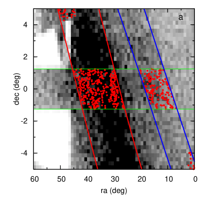
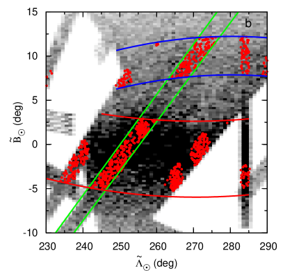
Figure 1: Spatial coverage of the photometric and spectroscopic observations across the Sgr stream around SDSS Stripe 82, in ra,dec coordinates (a) and in coordinates aligned with the Sgr stream (b). The greyscale density plots show the density of stars (0.2$\leq$g$-$i$\leq$0.45, 20.0$\leq$i$\leq$21.5) while the red points show the coverage of spectroscopic metallicities. Green lines indicate the extent of SDSS Stripe 82, while red and blue lines indicate the selection we adopt for the bright and faint stream respectively.

This is indeed the focus of our work: to study the detailed star formation history (SFH) of the Sgr stream in the Stripe 82 region, using data from the SDSS Data Release 10 (Ahn et al., 2014) and the Sloan Extension for Galactic Understanding and Exploration (SEGUE). Deep, MW foreground corrected CMDs will be used to determine the stellar population make-up of the stream in comparison to the populations of the parent Sgr galaxy. We utilise deep co-added photometry of the extensively covered Stripe 82 region to determine the photometric completeness of the single-epoch SDSS catalogs, allowing us to accurately model the observed CMDs (Annis et al., 2011). Furthermore, spectroscopic metallicities of individual stars are directly used in combination with the photometry to break the age-metallicity degeneracy and provide additional constraints on the age of the stellar populations, as described in de Boer et al. (2012a). We determine the detailed SFH for the bright and faint streams separately, to determine if both stream components consist of the same population mix of if they constitute two different streams.

The paper is structured as follows: in section 2 we present the selection of Sgr stars from the photometric SDSS survey, the MW foreground correction applied and the photometric completeness determination. The determination of the spectroscopic metallicity distribution of the Sgr streams is described in Section 3. Section 4 describes the determination of the SFH and discusses the specifics of fitting Sgr CMDs. The detailed SFH of the bright Sgr stream is presented in Section 5, followed by the SFH determination of the faint stream in Section 6. Finally, Sect. 7 discusses the results obtained from the comparison of both stream components and the implications from the SFH for the formation history of the Sgr dSph.

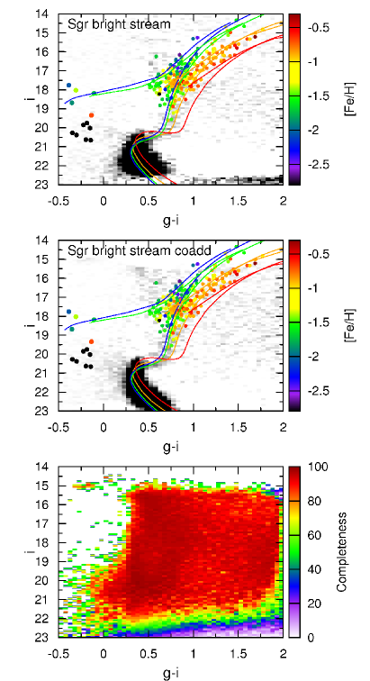
Figure 2: Comparison between extinction corrected single-epoch SDSS photometry (upper panel) and co-added photometry (middle panel) for the bright Sgr stream. Greyscale Hess diagrams show the density of stars in the CMD while the coloured points show spectroscopic observations of stream stars with colour indicating the metallicity. Several reference isochrones and HB tracks are also shown, corresponding to metal-poor (blue, [Fe/H]=-2.0, age=13 Gyr), intermediate (green, [Fe/H]=-1.5, age=12 Gyr) and metal-rich populations (orange: [Fe/H]=-0.8, age=8 Gyr, red: [Fe/H]=-0.3, age=5 Gyr) within Sgr. The photometric completeness is shown in the bottom panels, calculated by comparing the single-epoch and co-added data.

2 Sgr photometric data

To obtain accurate photometry of the Sgr stream in the Southern Stripe 82 we make use of SDSS Data Release 10 (Ahn et al., 2014). SDSS covered a wide area of the Sgr stream in the Southern hemisphere, with a 275 deg² degree region (equatorial Stripe 82) in particular being covered during numerous epochs. This region was covered during multiple runs resulting in deep co-added catalogs of stars reaching $\approx$2 magnitudes fainter than the SDSS single pass data (Annis et al., 2011). This extra depth is crucial for SFH analysis, as we can assume that the co-added catalog constitutes a 100% complete sample at the faintest magnitudes probed by single pass data. Therefore, a comparison between both catalogs can be used to estimate the photometric completeness in SDSS Stripe 82 data, a critical component of synthetic CMD analysis.

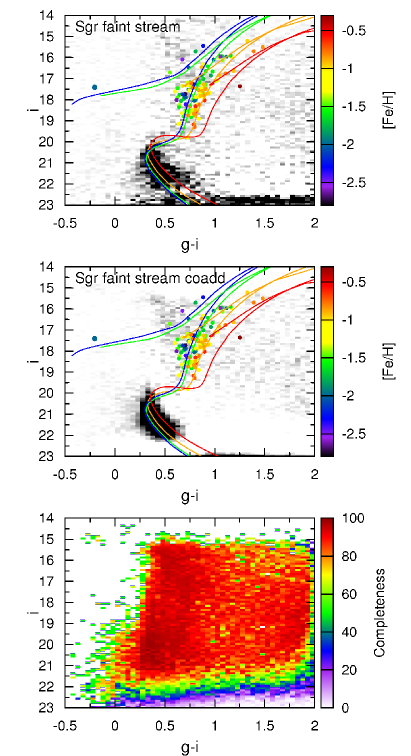
Figure 3: Same as Figure 2 but for the faint Sgr stream.

We select our Sgr photometric sample by making use of the prescriptions of Majewski et al. (2003) to transform equatorial ra and dec coordinates into heliocentric $\widetilde{\Lambda}_{\odot}$,$\widetilde{\mathrm{B}}_{\odot}$ coordinates that are aligned with the Sgr stream. Following the nomenclature of Belokurov et al. (2014), $\widetilde{\Lambda}_{\odot}$ increases in the direction of Sgr motion and $\widetilde{\mathrm{B}}_{\odot}$ points to the North Galactic pole. Figure 1 shows the density of main sequence (MS) stars in a region around Stripe 82 in ra, dec coordinates and coordinates aligned with the Sgr stream. Over-densities corresponding to the bright and faint Sgr streams are visible in Figure 1, highlighted by red and blue lines respectively. We combine these spatial cuts with the extent of Stripe 82 (green lines in Figure 1) to select our photometric sample of the Sgr bright and faint streams.

Due to the close proximity of the stream, there might be overlap between the bright and faint streams. To determine the effect of this overlap, we calculate the fraction of stars from one stream contained within the spatial selection of the other stream, under the assumption of Gaussian density distributions. We derive a contamination fraction of the bright stream within the faint stream region of 4%, which is large enough to be noticeable in the CMD. On the other hand, the contamination fraction of the faint stream on the bright stream is negligible at 0.05%. Following these calculations, we correct for the contamination effect on the faint stream, by subtracting the weighted CMD of the bright stream.

The CMDs determined in this way will contain stars of the Sgr stream as well as stars belonging to the MW at a wide range of distances and colours. These stars will contaminate the Sgr CMD and will be incorrectly fitted during the SFH determination using models at the distance of Sgr, leading to anomalously old and/or metal-rich populations in the SFH solution. To correct for the presence of these contaminants, we correct the photometric CMDs by subtracting a representative comparison CMD containing mostly MW stars. To select an appropriate correction region we consider that the MW is, to first order, symmetric around the Galactic plane and select stars from SDSS with the same Galactic longitude but latitude mirrored with respect to the Galactic plane. In this way we obtain a correction region containing the appropriate mix of disk and halo stars present at the Galactic longitude and latitude of our Sgr fields.

For the deep co-added photometry, we are constrained solely to data from Stripe 82 and therefore we cannot use a mirrored patch of sky in the foreground correction. Instead, we select a region between $-$10$<$ra$<$0 degrees within Stripe 82 for our decontamination field. This field corresponds to similar galactic latitude as our stream fields ($\delta$b$\leq$5 deg) but significantly different galactic longitude ($\delta$l$\geq$75 deg for the bright stream). Therefore, the stellar population mix of the MW foreground region is likely not the same as in our stream regions. To obtain an optimal subtraction of MW foreground halo stars (displaying similar colours as stream MSTO stars), we apply a colour shift to the foreground CMD before subtracting it from the stream CMD. The colour shift is derived by comparing the median g$-$i colour of MW halo turnoff stars in both CMDs using a selection box with 0.1$<$g$-$i$<$0.5, 18$<$i$<$19.5.

The Stripe 82 samples of Sgr stars span a total range of $\approx$20 degrees of angle along the stream. The stream displays a distance gradient of $\approx$5 kpc across this range, corresponding to a sizeable distance modulus difference of 0.35 mag. To correct for this variation of distance along the stream, we determine the distance of the bright and faint stream based on CMD distance indicators such as BHB, red clump (RC) and sub-giant branch (SGB) stars. Distances determined for both streams agree within the uncertainties with literature distance determinations by Niederste-Ostholt et al. (2010); Koposov et al. (2012). We correct for the presence of the distance gradient along both streams by interpolating the distance to each star in our sample and shifting it up or down in the CMD to a reference distance modulus of 17.5 mag (31.6 kpc) for the bright stream and 17.0 mag (25.1 kpc) for the faint stream, corresponding roughly to the observed distance to the stream within Stripe 82. Finally, to correct for the effect of dust extinction we also used extinction maps of Schlegel, Finkbeiner & Davis (1998) to determine the extinction toward each individual star within our sample and created extinction-free CMDs. The same distance and extinction correction procedure is also applied to the MW correction sample before subtracting it from the stream samples.

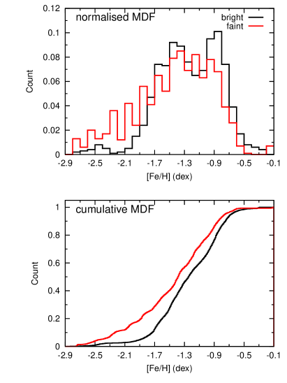
Figure 4: The metallicity distribution function of the bright and faint stream as obtained from spectroscopic observations. The top panel shows the normalised MDF, while the bottom panel shows the MDF in cumulative form.

The resulting MW corrected CMD of the bright stream is displayed in Figure 2. The deep co-added CMD for each region is also shown as well as the photometric completeness resulting from the comparison of both catalogs. Additionally, Figure 3 shows the same CMDs and completeness for the faint Sgr stream. The Sgr MS, SGB and lower RGB are clearly visible and traced by model isochrones at the distance of Sgr.

3 Sgr spectroscopic data

To obtain our Sgr spectroscopic sample, we make use of the SEGUE survey, which obtained medium-resolution spectra of stars covering a large portion of the sky, including many fields consistent with the Sgr stream (Yanny et al., 2009). The [Fe/H] and [$\alpha$/Fe] ratios for individual stars have been determined through detailed synthetic spectrum fitting using the SEGUE Stellar Parameter Pipeline (SSPP, Lee et al., 2008a, b; Allende Prieto et al., 2008; Smolinski et al., 2011; Lee et al., 2011). To select our sample of Sgr stars, we initially select stars based on their position on the sky, in the same way as the photometric sample. Additionally, we limit our sample to stars with robust stellar parameters and abundances using S/N$\geq$50 as well as spectroscopically confirmed giants using log $g$$\leq$3.5, 4300$\leq$T_eff$\leq$6000 K.

To reduce contamination from MW stars in the spectroscopic sample, we exploit the fact that the Sgr stream displays a clear signal in the $\widetilde{\Lambda}_{\odot}$ vs line-of-sight velocities V_GSR plane (Belokurov et al., 2014). In this plane, the Sgr-stream stars form a narrow sequence in each hemisphere, with velocities distinct from the MW. We use these sequences to refine our sample by selecting only stars consistent with the Sgr signal. To further decontaminate our sample we determine the distances to individual stars. Distances are obtained by selecting isochrone points with the correct g$-$i colour, and shifting their i-band magnitude to match the observations. We make use of the age-metallicity relation of Sgr globular clusters to determine the correct age at each metallicity (Forbes & Bridges, 2010). Subsequently, we pare our sample by keeping only those stars with distances consistent (to within 10 kpc) with the literature distance determinations to different branches of the stream from different distance indicators (Niederste-Ostholt et al., 2010; Koposov et al., 2012). Finally, we shift the spectroscopic stars of this sample according their distance to the same reference distance for the bright and faint stream as adopted for the photometric samples.

The sample of stars obtained in this way are displayed in Figure 1 as red points. In this work, we focus on SDSS Stripe 82 and therefore we only select those stars within the green lines in Figure 1. The stars in the spectroscopic sample are overlaid on the CMD in Figures 2 and 3 with colours representing the spectroscopic [Fe/H] abundance. The stars from our spectroscopic sample form a clear RGB as a continuation of the MS, SGB and RGB branches seen in the photometric CMD. Furthermore, a clear metallicity trend is visible in the CMD, consistent with the evolution of stellar populations in a relatively isolated system, indicating that our sample indeed consists of likely Sgr members.

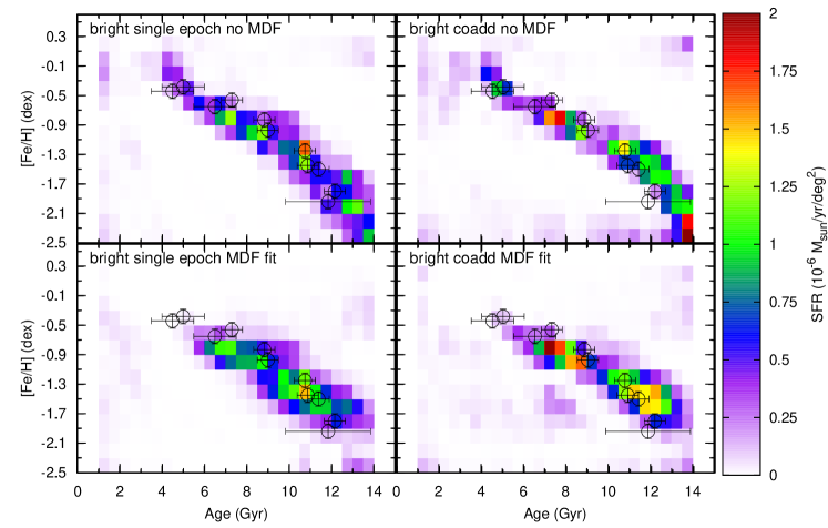
Figure 5: Full SFH solution as a function of age and metallicity for the bright Sgr stream within Stripe 82. Left panels show the solution derived from single-epoch photometric data, with and without MDF fitting, while the right panels shows solution derived from deep co-added data. The age and metallicity of globular clusters associated to the Sgr stream are also shown, as determined from deep CMD studies (Forbes & Bridges, 2010, and references therein).

To obtain a representative metallicity distribution function (MDF) for each stream, we must also take into account the spectroscopic sampling efficiency of SDSS/SEGUE, which consists of different surveys with different depths and target selections. Therefore, we correct for the completeness of spectroscopic stars as a function of position in the CMD. For each SDSS plate we take all stars (including MW foreground) with SDSS photometry and all stars with spectroscopy, by sampling the area of each target plate (with radius 1.49 degrees). Those two samples are binned in the CMD space and the ratio of the two CMD densities tells us the completeness of the SDSS spectroscopy relative to the photometry , which is assumed to be complete at the sampled magnitudes.

These completeness measures are then used to weight the importance of each star in the observed MDF for the bright and faint streams. Finally, we also correct the spectroscopic MDF of the faint stream for the effect of contamination from the bright stream, by subtracting a weighted bright stream MDF as outlined in Section 2. The spectroscopic MDFs obtained in this way are shown in Figure 4, highlighting the differences between both streams. The cumulative MDF clearly shows that the faint stream is composed of more metal-poor populations than the bright stream, with almost no stars more metal-poor than [Fe/H]=$-$0.9.

4 SFH method

The SFH of the Sgr streams will be determined using the routine Talos, which employs a synthetic CMD method (e.g., Tosi et al., 1991; Tolstoy & Saha, 1996; Gallart et al., 1996; Dolphin, 1997; Aparicio, Gallart & Bertelli, 1997). This technique determines the SFH by comparing the observed CMDs to a grid of synthetic CMDs using Hess diagrams (plots of the density of observed stars), taking into account photometric error and completeness. Uniquely, Talos simultaneously takes into account the photometric CMD as well as the spectroscopic MDF, providing direct constraints on the metallicity of stellar populations to obtain a well-constrained SFH. We refer to de Boer et al. (2012a) for a detailed description of the routine and performance tests.

To determine the SFH of Sgr, we assume a wide range of possible ages and metallicities to avoid biasing the solution by our choice of parameter space. For the metallicity, a lower limit of [Fe/H]=$-$2.5 dex is assumed, which is the lowest available in the Dartmouth library used in this work (Dotter et al., 2008). We do not expect this to lead to a bias in the SFH results since very few stars in Sgr are expected to have low metallicities. An upper limit of [Fe/H]=0.3 dex is assumed for the metallicity based on spectroscopic measurements of the metallicity in central body of Sgr (Smecker-Hane & McWilliam, 2002; Carretta et al., 2010; McWilliam, Wallerstein & Mottini, 2013). The $\alpha$-element abundance of the isochrones used is varied with metallicity according to the observed [$\alpha$/Fe] distribution of the Sgr stream, ranging from [$\alpha$/Fe]=$-$0.2 to [$\alpha$/Fe]=0.4 (de Boer et al., 2014). For the age limits, we assume a maximum age of 14 Gyr for the age of the Universe and considered a range of ages between 0.25 (the youngest age available in the isochrone set used) and 14 Gyr old, with a uniform bin size of 0.5 Gyr.

The SFH is determined using the (i, g$-$i) CMD to make use of a large dynamic range in the CMD while sticking to the well studied g and i bands. The SFH fitting is restricted to the MS and lower RGB regions, using CMD limits of $-$0.3$<$g$-$$i<$1.3 and 18$<$i$<$22 for the bright stream and $-$0.3$<$g$-$$i<$1.3 and 17.5$<$i$<$21.5 for the faint stream. The bright magnitude cut excludes the heavily contaminated upper RGB and MW thick disk regions, while the faint end of the CMD is truncated to avoid fitting the SFH in regions where the photometry becomes less reliable in SDSS data (see Figure 2).

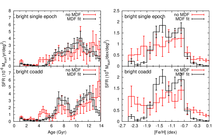
Figure 6: Star formation rates projected onto age (star formation history, left) and metallicity (chemical evolution history, right) of the bright Sgr stream. Solutions from single-epoch data are shown in the top panels, while co-add photometry solutions are shown in the bottom panels.

5 Star formation history of the bright stream

The star formation history of the Sgr bright stream is derived using the single-epoch SDSS data presented in Figure 2. The SFH solution is obtained both with and without fitting the spectroscopic MDF, to assess the effect of the MDF constraints on the derived stellar populations. Furthermore, to study the effects of data quality and depth on the SFH, we also make direct use of the deep co-added photometry available in SDSS Stripe 82. Therefore, we also determine the SFH from the co-add photometry for the bright stream, under the assumption that the photometry is 100% complete down to the faint CMD limit of i=22.

Figure 5 shows the SFH solutions as obtained from both the single-epoch (left panels) and deep co-added SDSS photometry (right panels) for the Sgr bright stream. Solutions obtained with and without fitting the MDF are shown in the bottom and top panels respectively, to highlight the differences in the SFH associated to the constraints from the spectroscopic MDF. The star formation rate (SFR) is normalised by spatial extent using a total area of 39.4 deg² for the bright stream as shown in Figure 1.

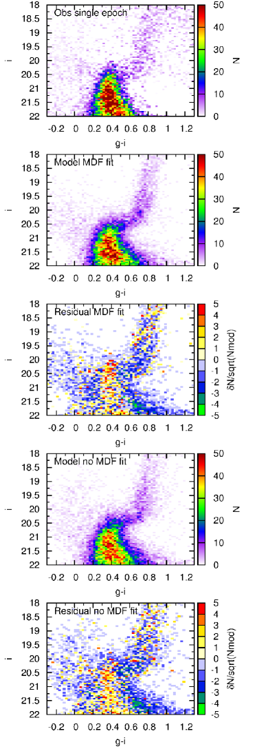
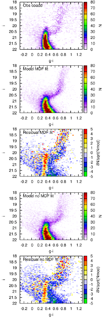
Figure 7: Observed and best-fitting CMDs for the bright stream of Sgr, with and without MDF fitting. The middle and bottom rows show the difference between the observed and best-fit CMDs, expressed as a function of the uncertainty in each CMD bin.

By projecting the SFR values onto one axis we obtain the SFR as a function of age (SFH) or metallicity (chemical evolution history, CEH), which are shown in Figure 6. The error bars indicate the uncertainty on the SFR as a result of different CMD and parameter grids (as described in de Boer et al. (2012a)). The SFH and CEH display the rate of star formation at different ages and metallicities over the range of each displayed bin in units of solar mass per year or dex respectively. The total stellar mass in this section of the stream can be computed by multiplying the star formation rates by the range in age or metallicity of each bin and multiplying by the total spatial area.

To assess the goodness of fit of the SFH solutions, Figure 7 shows a comparison between the observed and synthetic (i, g$-$i) CMDs of the bright stream for the single-epoch data (left panels) and the deep co-added data (right panels). The middle and bottom panels of Figure 7 show the fit residuals in each bin in terms of Poisson uncertainties. Furthermore, the goodness of fit can also be assessed by comparing the metallicities of stars in the best-fit SFH model on the upper RGB to the observed MDF as shown in Figure 8 with and without MDF fitting.

5.1 Single-epoch data

The SFH solutions derived from single-epoch photometry allow us to study the Sgr stream populations using data of a depth and quality as found throughout the SDSS survey. In this way, we can study the formation history of Sgr with a precision which can also be achieved at different angles along the stream within SDSS.

To assess the goodness of the derived fit, we compare the observed and synthetic CMDs of the bright stream in the left panels of Figure 7. Comparison between these CMDs indicates that the SFH solutions shown in Figures 5 and 6 constitute an overall good fit of the data, with CMDs largely consistent within 3 sigma in most bins for both the solutions with and without taking into the MDF. The synthetic CMDs correctly reproduce all evolutionary features in the lower CMD, including the location and spread of the MSTO, SGB and faint RGB as well as the presence of younger populations above the nominal SGB. However, Figure 7 also shows features that do not fit as well, such as the presence of red RGB stars which could be fit to residual foreground stars and stars red-ward of the faint MS.

Comparison between the derived synthetic MDF for each solution (see Figure 8) and the observations shows a good fit for the solution with MDF fitting, which is expected since the MDF was used directly as an input. For the solution without MDF fitting, the best-fit model is broadly consistent with the observations, with the mean peak at similar metallicities. However, the distribution of more metal-poor stars is much broader than the observations, extending all the way to [Fe/H]=$-$2.3 instead of peaking at [Fe/H]=$-$1.5. The origin of this excess of metal-poor stars in the model is not clear, but could be related to the similarity between metal-poor models in the CMD at the MSTO level, leading to a smearing out of metallicity information. Furthermore, it is also possible that these stars are present in the Sgr stream, but not fully sampled in the observed MDF. A slight excess of metal-rich stars is also visible, which might be linked to stellar populations fit to the red foreground stars seen in Figure 7.

The best-fit SFH solution for the Sgr bright stream is characterised by a well-defined sequence in age-metallicity space (see Figure 5) starting from old, metal-poor populations ([Fe/H]$\approx$$-$2.5, age$\approx$14 Gyr) and extending to intermediate ages ($\approx$5 Gyr) with high metallicities ([Fe/H]=$-$0.7). This sequence is relatively narrow, indicating that Sgr experienced metal enrichment under relatively isolated conditions without strong inhomogeneous mixing. The sequence of Sgr populations displays a change of slope in age-metallicity space at an age$\approx$12-13 Gyr and metallicity [Fe/H]$\approx$$-$1.5. The location of this change in slope of the age-metallicity relation (AMR) is roughly consistent with that of the $\alpha$-element knee observed by de Boer et al. (2014), indicating it could be linked to the onset of supernovae type Ia contributing to the metal enrichment of Sgr.

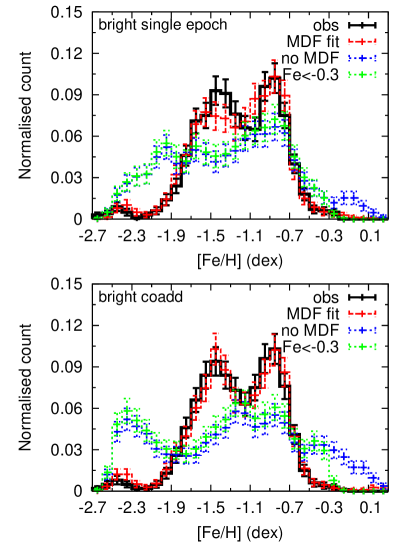
Figure 8: Normalised metallicity distribution function (as sampled on the bright RGB) for the Sgr bright stream from deep co-added (top) and single-epoch (bottom) photometry, with and without MDF fitting in the SFH derivation. The observed MDF is shown as black lines, while the best-fit result from the SFH derivation is shown in red and blue for solution respectively with and without MDF fitting. The green line indicates the MDF derived without MDF fitting after applying a cut on the possible metallicity of stream member stars. The error bars indicate the uncertainties on the MDF due to uncertainties on the SFH for the model and due to Poisson errors for the observations.

To compare the results obtained for the Sgr stream in Stripe 82 to results for Sgr across a wider spatial range, we compare our SFH to the stellar population parameters of 11 globular clusters (GCs) associated to the Sgr stream, as determined from very deep CMD studies (Forbes & Bridges, 2010, and references therein). The age and metallicity (and uncertainties) are shown as large circles with error bars overlaid on the Sgr stream results in Figure 5. The sequence traced out by Sgr populations is consistent with the parameters determined for the GCs indicating that the SFH obtained here is indeed a good representation of Sgr populations.

Results obtained with and without the spectroscopic MDF fitting show an overall good agreement in recovering the same sequence in age-metallicity space. However, the SFH results without including the MDF show the presence of very metal-rich populations ([Fe/H]$\geq$$-$0.3), which are not recovered in the spectroscopic metallicities of stream stars at this location on the sky. The red reference isochrone in Figure 2 traces the location in the CMD of the metal-rich populations seen in Figure 5 and shows these are inconsistent with the observed upper RGB of Sgr if given a significant SFR. Therefore, these populations are likely the result of fitting to red excess foreground stars and do not represent genuine Sgr populations. To assess the effect of these population on the synthetic MDF, the green, dotted line in Figure 8 shows the synthetic MDF as obtained without including stars with metallicities above [Fe/H]=$-$0.3. This MDF provides a better fit to the observed MDF at high metallicities, while metal-poor stars are still spread over a wide range of metallicities.

The SFH as a function of age and metallicity shows that Sgr displays high SFR across a large range of ages, with several periods of increasing and decreasing SFR. Below an age of $\approx$6 Gyr the SFR declines rapidly, indicating the end of star formation in the part of Sgr associated to the stream at this location. This might be related to the accretion of Sgr by the MW, which is expected to strip the dwarf galaxy of its remaining gas and truncate star formation. The stellar populations in the Sgr stream span a range of metallicity between [Fe/H]$\approx$$-$2.5 and [Fe/H]=$-$0.5 without a strong peak at metal-poor metallicities seen in many other dwarf galaxies (e.g., de Boer et al., 2012a, b). This lack of a dominant metal-poor component might be related to the large mass of Sgr, resulting in efficient metal enrichment at early times or this section of stream being stripped from the more central parts of the progenitor, dominated by more metal-rich stars.

The distinct periods of star formation in Figures 5 and 6 as constrained using stars from the bottom of the CMD are in good agreement with evolved population features in the bright CMD (RGB, HB and RC). The position and slope of the RGB as traced by the isochrones shown in Figure 2 agrees with the spectroscopic metallicities shown in Figure 2. This indicates that these populations provide a good fit to both evolved and non-evolved CMD indicators. Results obtained with and without MDF fitting are consistent within the errors, except for the presence of very metal-rich populations in the solution without spectroscopic MDF.

5.2 Deep co-added data

Due to the better quality of the deep SDSS co-added data, we achieve a higher S/N of the Sgr stream and smaller photometric errors at the level of the nominal MS turnoff (see Figure 2). This allows us to determine the effects on the SFH related to the depth and data quality of SDSS photometry.

The CMD residuals in the right panels of Figure 7 once again show an overall good fit of the synthetic CMDs for both the solutions with and without taking into account the MDF. However, a strong positive residual is present at g-i$\approx$0.3, which is consistent with the blue edge of the CMD area affected by MW foreground contamination. Therefore, this residual could be the result of a different population mix between the stream and foreground regions, which do not sample identical Galactic latitude and longitude within Stripe 82. Furthermore, the sharp blue edge of the residual could also indicate a difference in extinction not accounted for in dust maps or different photometric error distribution. Furthermore, the CMD residuals also show the presence of several populations clearly inconsistent with the main locus of Sgr stars, such as fits to very red foreground stars or blue BSS stars. These populations show up as low level SFR in Figure 5 as metal-rich ([Fe/H]$<$$-$0.3), old populations or stars with very young ($<$2 Gyr) ages.

The SFH as obtained from the deep co-added data is overall in good agreement with the SFH obtained from single-epoch data. The well-defined sequence in age-metallicity space is also visible in the co-added data and consistent with the shallower data. The sequence appears more defined and narrower in the deep photometry, due to the better data quality, resulting in better age resolution. Comparison between the deep and shallow data shows that the single-epoch SDSS data quality is sufficient to correctly recover the age-metallicity relation of the Sgr stream, giving further confidence to the results of Section 5.1.

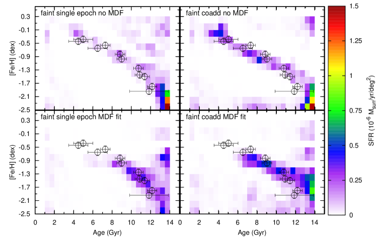
Figure 9: Full SFH solution as a function of age and metallicity for the faint Sgr stream within Stripe 82 (see Figure 1), with and without MDF fitting in the SFH derivation. Left panels show the solution derived from single-epoch photometric data, while the right panels shows solution derived from deep co-added data.

The SFH projected on age and metallicity also shows similar features as seen for single-epoch data in Figure 6, with strong star formation from ancient times ($>$10 Gyr) and a strong decline in SFR at $\approx$6 Gyr ago. Results obtained with the inclusion of MDF fitting for both single-epoch and co-added data show peaks at similar times in Figure 6 consistent within the uncertainties, although results from co-added photometry are shifted slightly to older ages. The co-added SFH shows a drop in SFR around an age of 9 Gyr, which is not reproduced in the top panels of Figure 6. The most likely explanation for this is the difference in data quality between both datasets, resulting in a worse age resolution in the single-epoch data and smoothing out the SFR peaks to fill the gap at 9 Gyr. Furthermore, this feature might also be related to the broad SGB in Figure 7, showing gaps in the density distribution. Unfortunately, this region of the CMD suffers from poor MW foreground decontamination, which may affect the SFH results.

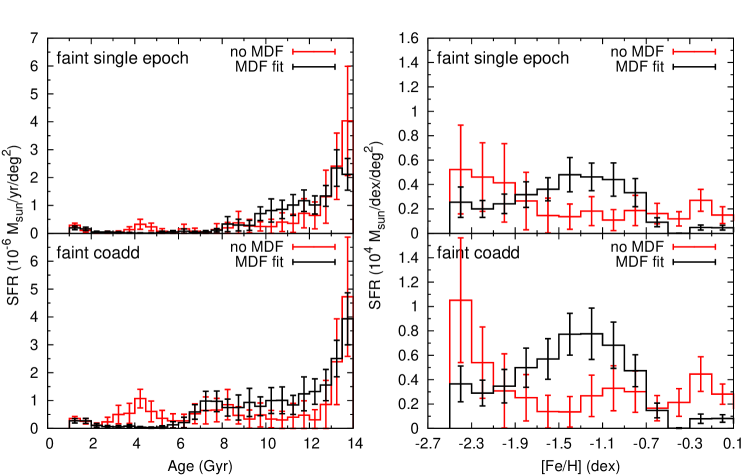
Figure 10: Star formation rates of the faint stream projected on age (star formation history, left) and metallicity (chemical evolution history, right). Solutions from single-epoch data are shown in the top panels, while co-add photometry solutions are shown in the bottom panels.

6 Star formation history of the faint stream

To study the properties of the faint Sgr stream, we employ the same procedure as used in Section 5. To compare the results of the faint stream to those of the bright stream, we use the same range of stellar populations in the fitting with the same age and metallicity resolution. The faint stream SFH is fit using the (i, g$-$i) CMD, with the same CMD limits as assumed in the fitting of the bright stream. However, due to the lower number density of stars in the faint stream, the colour and magnitude bin size has been doubled to achieve enough signal in each CMD bin. The fitting routine once again makes use of completeness information based on the comparison between deep co-added and single-epoch photometry as shown in Figure 3.

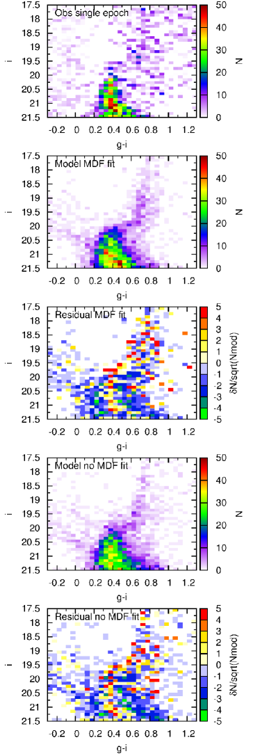
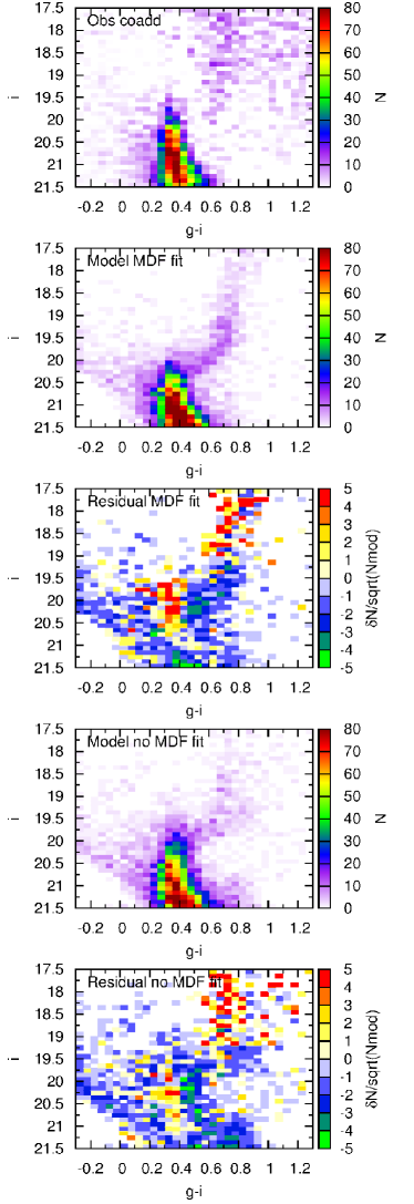
Figure 11: Observed and best-fitting CMDs for the faint Sgr stream from single-epoch (left) and deep co-added (right) photometry, with and without MDF fitting. The middle and bottom rows show the difference between the observed and best-fit CMDs, expressed as a function of the uncertainty in each CMD bin.

6.1 Single-epoch data

The best-fit SFH solution for the faint Sgr stream is shown in Figure 9 as a function of age and metallicity. Figure 9 also shows the solution as obtained without fitting the spectroscopic MDF. The SFR values are normalised by the spatial area of each region of the stream, using a spatial area of 24 deg² for the faint stream in Stripe 82. Furthermore, Figure 10 shows the results for the SFH and CEH by projecting the SFR onto age and metallicity respectively, in units of solar mass per year and dex respectively.

Comparisons between the observed (i, g$-$i) CMD and the best-fit CMD obtained from the SFH are shown in Figure 11 for each region, along with the residual in each bin in terms of Poisson uncertainties. To further asses the quality of the fits, Figure 12 shows the observed MDFs on the upper RGB in comparison to the synthetic MDFs inferred from the SFH solution with and without MDF fitting. Once again, for the solution including spectroscopic MDF fitting, the good fit is expected given that the MDF is used as input.

The CMD residuals indicate that the SFH solution produces an overall good fit of the observed CMDs, without any obvious systematic residuals. The synthetic CMDs reproduce the MS and MSTO at the right location and produce an SGB and lower RGB consistent with the observed CMD as sampled from both photometric and spectroscopic stream members (see Figure 3). Due to the lower intrinsic signal of the faint stream, the sampling of the stellar evolution features is less than for the bright stream, leading to greater uncertainties in the SFH. Furthermore, there is a stronger effect of incomplete MW foreground correction, especially visible red-ward of the nominal MSTO and SGB (g$-$i$\approx$0.8, i$\approx$20.5). Therefore, Figure 9 shows the presence of more anomalous populations with higher metallicities and older ages (driving isochrones to redder colours) compared to the Sgr stellar population sequence.

The SFH results presented in Figures 9 and 10 show that the Sgr faint stream displays a sequence in age-metallicity space similar to that observed in the bright stream (see Figure 5). This sequence is also compatible with the age-metallicity relation traced out by GCs associated to the Sgr dwarf galaxy, although the faint stream does not sample the same extent of the sequence as the bright stream. Instead, the faint stream samples the older, more metal-poor part of the sequence, being comprised mostly of stars with [Fe/H]$<$$-$1 and age$>$9 Gyr. This is also visible in Figure 10, showing that star formation peaks at ancient ages.

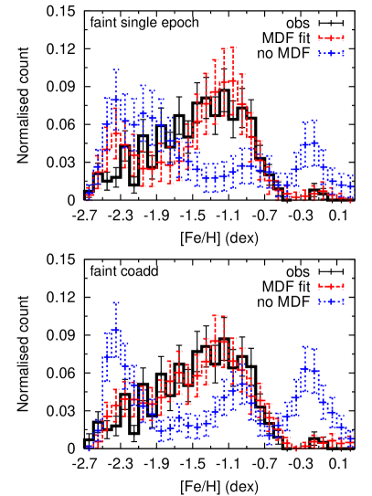
Figure 12: Normalised metallicity distribution function for the Sgr faint stream, with and without MDF fitting in the SFH derivation. Deep co-added solutions are shown in the top panel and single-epoch solutions in the bottom panel. The observed MDF is shown as black lines, while the best-fit result from the SFH derivation is shown in red and blue for solution respectively with and without MDF fitting. Error bars indicate the uncertainties on the MDF due to uncertainties on the SFH for the model and due to Poissonian errors for the observations.

The SFH results obtained with and without MDF fitting both trace the same age-metallicity sequence. However, the SFH peak in the solution without MDF fitting is strongly peaked at metal-poor metallicities and is more spread out in age-metallicity space than the solution with MDF fitting. Comparison to Figure 11 shows that the solution without MDF indeed displays a dominant blue SGB and RGB consistent with metal-poor, old populations, while the MDF fit produces a redder RGB and SGB due to more metal-rich populations. Furthermore, best-fit models without MDF result in a wide range in colour at faint magnitudes, with fits to stars associated to MW halo contamination. Due to the sparse sampling of the evolved features in the CMD and the strong MW contamination it is unclear which of these solutions fits the CMD best. Deeper CMDs or wider angle along the stream are needed to increase the S/N of the stream signal to unambiguously determine the presence of these features.

Comparing the results from Figures 5 and 9 shows that both the bright and faint stream in Stripe 82 are drawn from the same stellar population mix present elsewhere in the stream and in the progenitor. However, the populations in the faint stream are not consistent with those of the bright stream, arguing in favour of a scenario where the faint stream consists of material stripped from the outskirts of the Sgr dwarf at an earlier epoch.

6.2 Deep co-added data

To obtain a better picture of the faint stream stellar populations, we once again make use of the deep co-added photometry of Stripe 82. Due to the deeper data we achieve a higher S/N not only for the MS region of the CMD but also for the MSTO and SGB regions, crucial for disentangling the ages of the stellar populations.

Figures 9 and 10 present the best-fit SFH solution for the faint Sgr stream from co-added photometry. The SFR as a function of age and metallicity is shown in Figure 9 in comparison to single-epoch results, while Figure 10 displays the SFR projected onto the age and metallicity axes respectively. The comparison between observed and synthetic CMD is shown in the right panels of Figure 11 for the solution with and without MDF fitting, along with associated residuals. Additionally, the comparison between observed and best-fit MDFs is shown in Figure 12.

Comparison between the single-epoch and co-added CMDs in Figures 11 shows that the MW foreground contamination is greatly reduced around the MSTO/SGB region, leading to a better determination of the ages of the faint stream populations. Similar to results obtained for the bright stream, systematic residuals are visible in Figure 11 above the nominal MSTO and at the faint edge of the CMD, for both the solutions with and without taking into the MDF. The location of the positive residuals coincides with a region of the CMD strongly affected by MW foreground correction. Due to the limited choice of foreground region available within the deep co-added data, it is likely that the MW stellar population in between the foreground and stream regions is not fully consistent, which can account for the residuals in Figure 11.

The SFH of the faint stream as obtained from the co-added data is consistent with the single-epoch SFH shown in Figures 9 and 10. Similar sequences are visible in both solutions, with peaks at similar age and metallicity. Due to the better data quality of the deep data, the sequence is more defined in the co-added data and shows less effects of populations fit to residual foreground stars. Results for the SFH projected on age and metallicity as well as the spectroscopic MDF are also consistent to within the error bars. The SFH is dominated by old star formation at relatively metal-poor metallicities ([Fe/H]$<$$-$1.5) but also shows a peak at age $\approx$8 Gyr ago, slightly older than single-epoch results.

The synthetic MDF derived from the best-fit SFH solution is in better agreement with the observed MDF given the generous error bars, unlike the results for single-epoch data. This metal-rich peak is related to the burst of star formation $\approx$8 Gyr ago, similar to what was observed for the bright stream in Figure 5.

7 Conclusions and discussion

In this work, we present the first detailed quantitative study of the stellar populations of the Sgr trailing stream, using photometric and spectroscopic observations from the SDSS surveys. By modelling the available data, we infer the Sgr SFH and MDF as displayed by the stars in a portion of the (bifurcated) trailing tail of the galaxy. Such detailed SFH and MDF of the bright and faint stream components within the Stripe 82 region provide new constraints of the model of the dwarf disruption. The results of our study can be summarised as follows.

• As displayed in Figures 7 and  11, the models of the CMD density distribution appear sensible and reproduce the bulk of the Sgr stellar populations as observed by the SDSS in the Southern Hemisphere. There is, however, a small amount of positive residuals, in particular at the MSTO colour. This systematic mismatch is possibly due to a small level of asymmetry in the Galactic disk and halo, and therefore was introduced at the foreground subtraction stage. Alternatively, it can not be ruled out that a slightly misjudged extinction could cause such an artificial pile-up.

• Solutions with MDF and without MDF look generally consistent, however fits without MDF constraints are clearly degenerate and appear to lead to biased inference as to the SFH details (see Figures 5-12). For example, solutions derived without including MDF fitting produce a more extended sequence reaching all the way up to solar metallicity, which is not supported by the spectroscopic observations. Comparison with the observed CMD (see red isochrone in Figure 2) shows that populations with these parameters are not observed in great number on the red side of the RGB locus or in the sample of kinematic member stars, indicating that these populations should not be present with substantial star formation rates. The presence of these populations could be a result of fitting models to residual foreground stars red-ward of the nominal RGB. However, the age and metallicity of the populations is consistent with a picture of steady chemical enrichment in an isolated environment and does occur in the Sgr dwarf galaxy as traced by the distribution of GCs. To improve the interpretation of these populations, we need to sample a larger portion of the streams, to increase the relative S/N of these stream populations.

  Additionally, comparison of results derived with and without MDF fitting shows that solutions without MDF fitting produce a systematically higher SFR in populations with [Fe/H]$>$$-$2. This is due to the lack of stars with such low metallicities in the spectroscopic MDF, as shown in Figures 8 and 12. This lack of metal-poor stars could be a result of the efficient enrichment in a massive dwarf galaxy such as Sgr, quickly increasing the metallicity of the interstellar medium from which subsequent generations of stars are formed. On the other hand, the region of the CMD occupied by metal-poor stars is heavily contaminated by foreground stars, leading to a larger fraction of fibers being assigned to foreground stars than for metal-rich stars,in the case of random spectroscopic fiber assignment. This type of completeness cannot be corrected for given the inherently unknown distribution of foreground and background populations. A better spectroscopic sampling of the Sgr stream is necessary to unambiguously determine the fraction of metal-poor stars within the Sgr stream.

• Both bright and faint stream components show a tight sequence in the plane of Age vs [Fe/H] as shown in Figures 5 and 9 indicating that star formation within Sgr took place in a well-mixed medium, homogeneously enriched in metals over $\approx$8 Gyr. The tight sequence starts from old, metal-poor populations and extends to a metallicity of [Fe/H]$\approx$$-$0.7 at an age of $\approx$5 Gyr before star formation terminates. The SFH (see Figures 6 and 10) confirms the extended formation history of the progenitor Sgr dwarf galaxy and quantifies the strength and stellar population make-up of each star formation episode. The tight sequence observed in the bright stream is also reproduced in the faint one, although the lower S/N of the stream results in the presence of more anomalous populations due to residual foreground stars. Star formation in the faint stream is dominated by metal-poor populations, with a SFH mostly composed of stars $>$10 Gyr old (see Figure 10). Therefore, the faint stream appears composed of a simpler stellar population mix than the bright stream.

• To compare the SFH of the streams to the overall SFH of Sgr, Figures 5 and 9 show the age and metallicity of GCs associated to the Sgr dwarf galaxy (Forbes & Bridges, 2010). The GCs trace out the same tight sequence in age and metallicity space, indicating that the sequence observed in both streams is consistent with Sgr populations present elsewhere in the stream and main body. Therefore, both streams are consistent with being drawn from the mix of populations associated to Sgr.

• We can use the SFH derived here for both stream components to study the formation history of the parent Sgr dwarf galaxy. It is clear from Figure 6 that the Sgr galaxy has undergone an extended formation history, with multiple peaks in SFR. This indicates that Sgr formed stars over a substantial period of star formation of at least 7 Gyr. The MDF of the bright stream also shows strong evidence for a bi-modality with peaks at [Fe/H]$\approx$-1.5 and -1.

  The faint stream, on the other hand, displays neither clear peaks in the SFH nor additional bumps in the MDF. We conclude again (bearing in mind that the faint stream data possesses lower S/N), that the fainter stream has experienced a less eventful star formation history and contains a simpler population mix.

• In the bright stream, star formation rates drop rapidly around $\approx$5-7 Gyr ago; this also corresponds to the last substantial star formation activity in the faint stream. This shutdown of star formation could be caused by the infall of Sgr into the MW potential, coinciding with stripping of gas from the outskirts of the system, from which the streams were formed.

• The sequence of Sgr populations displays a change of slope in age-metallicity space at an age between 11-13 Gyr and metallicity [Fe/H]$\approx$$-$1.5. The location of this change in slope of the age-metallicity relation (AMR) is consistent with that of the $\alpha$-element knee observed by de Boer et al. (2014), indicating that supernovae type Ia started contributing noticeably to the abundance pattern $\approx$1-3 Gyr after the start of star formation in Sgr.

• There is one additional significant difference between the stellar population properties of the bright and the faint streams. As illustrated in the Figure 4, the faint stream seems to lack a significant metal-rich component with [Fe/H]$>$-0.9, the population easily discernible in the bright stream.

• Finally, we would like to point out that the analysis has been carried out using both single-epoch and stacked SDSS photometry. It is re-assuring to see that the results of modelling of each dataset are consistent with each other. However, deeper data clearly provides better constraints on the SFH: the age-metallicity sequence is much tighter, while the peaks corresponding to SFH activity are more significant.

Overall, we believe that this pilot study has convincingly demonstrated that SFH and MDF inference can be obtained for low-surface brightness structures in the Galactic halo. Studies such as this one will greatly benefit from future deep wide-field surveys such as LSST, which will be able to tap into the large number of MS stars in both stream components, leading to more accurate inferred distances and stellar population parameters. Apart from the obvious necessity for a deeper wide-area survey data, we would also like to emphasise two potential routes for improvement. First, to avoid biases caused by improper foreground subtraction, analysis of the broad band stream photometry and spectroscopy could proceed simultaneously with the foreground modelling. For the Galaxy, this of course would require simultaneous fitting of the volume density as well as the CMD. Second, small but noticeable CMD density residuals displayed above could potentially be a sign of changing stream distance, distance spread or the presence of additional stream components. Therefore, rather than fixing the sub-structure’s distance and distance spread, as well as the number of unrelaxed fragments along the line-of-sight, the model can be relaxed to include these as free parameters.

The results of our analysis bear implications for the modelling of the Sgr disruption. Interestingly, as summarised earlier, the star formation activity, inferred with the stream stars, appears curtailed $\approx$ 5-7 Gyr ago. Typically, in stellar stream modelling, the total disruption time is the least constrained “nuisance” parameter which can play, however, a very important role. For example, in case of the Sgr dwarf, if the tidal debris have orbited within the MW for sufficiently long time, the global stream parameters, such as apsidal and orbital plane precession angles could be affected by the subsequent material accretion. As far as the differences between the bright and the faint stream components are concerned, we i) prove that the Sgr dwarf is likely the progenitor of the faint component as well as the bright one, and ii) present strong evidence that the star-formation and chemical enrichment proceeded in a similar fashion for each part of the bifurcation. However, we also confirm earlier claims of Koposov et al. (2012) of a subtle variation in the MDF of the faint stream as compared to the bright. According to our analysis, the faint component of the trailing stream displays a simpler mix of stellar populations dominated by old metal poor stars and lacks a strong metal-rich ingredient obviously present in the bright tail. Viewed naively, such differences in stellar populations can perhaps be explained if the faint stream was produced by the material stripped i) earlier and ii) from the outskirts of the dwarf.

References

- Ahn et al. (2014) Ahn C. P. et al., 2014, ApJS, 211, 17
- Allende Prieto et al. (2008) Allende Prieto C. et al., 2008, AJ, 136, 2070
- Annis et al. (2011) Annis J. et al., 2011, ArXiv e-prints
- Aparicio, Gallart & Bertelli (1997) Aparicio A., Gallart C., Bertelli G., 1997, AJ, 114, 669
- Bellazzini et al. (2006a) Bellazzini M., Correnti M., Ferraro F. R., Monaco L., Montegriffo P., 2006a, A&A, 446, L1
- Bellazzini et al. (2008) Bellazzini M. et al., 2008, AJ, 136, 1147
- Bellazzini et al. (2006b) Bellazzini M., Newberg H. J., Correnti M., Ferraro F. R., Monaco L., 2006b, A&A, 457, L21
- Belokurov (2013) Belokurov V., 2013, New A Rev., 57, 100
- Belokurov et al. (2014) Belokurov V. et al., 2014, MNRAS, 437, 116
- Belokurov et al. (2006) Belokurov V. et al., 2006, ApJ, 642, L137
- Carretta et al. (2010) Carretta E. et al., 2010, A&A, 520, A95
- de Boer et al. (2014) de Boer T. J. L., Belokurov V., Beers T. C., Lee Y. S., 2014, MNRAS, 443, 658
- de Boer et al. (2012a) de Boer T. J. L. et al., 2012a, A&A, 539, A103
- de Boer et al. (2012b) de Boer T. J. L. et al., 2012b, A&A, 544, A73
- Deason, Belokurov & Evans (2011) Deason A. J., Belokurov V., Evans N. W., 2011, MNRAS, 416, 2903
- Deason et al. (2014) Deason A. J., Belokurov V., Koposov S. E., Rockosi C. M., 2014, ApJ, 787, 30
- Dolphin (1997) Dolphin A., 1997, New Astronomy, 2, 397
- Dotter et al. (2008) Dotter A., Chaboyer B., Jevremović D., Kostov V., Baron E., Ferguson J. W., 2008, ApJS, 178, 89
- Fellhauer et al. (2006) Fellhauer M. et al., 2006, ApJ, 651, 167
- Forbes & Bridges (2010) Forbes D. A., Bridges T., 2010, MNRAS, 404, 1203
- Freeman & Bland-Hawthorn (2002) Freeman K., Bland-Hawthorn J., 2002, ARA&A, 40, 487
- Gallart et al. (1996) Gallart C., Aparicio A., Bertelli G., Chiosi C., 1996, AJ, 112, 1950
- Gibbons, Belokurov & Evans (2014) Gibbons S. L. J., Belokurov V., Evans N. W., 2014, ArXiv e-prints
- Ibata, Gilmore & Irwin (1995) Ibata R. A., Gilmore G., Irwin M. J., 1995, MNRAS, 277, 781
- Jurić et al. (2008) Jurić M. et al., 2008, ApJ, 673, 864
- Koposov et al. (2012) Koposov S. E. et al., 2012, ApJ, 750, 80
- Koposov et al. (2015) Koposov S. E., Belokurov V., Zucker D. B., Lewis G. F., Ibata R. A., Olszewski E. W., López-Sánchez Á. R., Hyde E. A., 2015, MNRAS, 446, 3110
- Law & Majewski (2010) Law D. R., Majewski S. R., 2010, ApJ, 714, 229
- Lee et al. (2011) Lee Y. S. et al., 2011, AJ, 141, 90
- Lee et al. (2008a) Lee Y. S. et al., 2008a, AJ, 136, 2022
- Lee et al. (2008b) Lee Y. S. et al., 2008b, AJ, 136, 2050
- Majewski et al. (2003) Majewski S. R., Skrutskie M. F., Weinberg M. D., Ostheimer J. C., 2003, ApJ, 599, 1082
- Martínez-Delgado et al. (2007) Martínez-Delgado D., Peñarrubia J., Jurić M., Alfaro E. J., Ivezić Z., 2007, ApJ, 660, 1264
- McWilliam, Wallerstein & Mottini (2013) McWilliam A., Wallerstein G., Mottini M., 2013, ApJ, 778, 149
- Monaco et al. (2005) Monaco L., Bellazzini M., Bonifacio P., Ferraro F. R., Marconi G., Pancino E., Sbordone L., Zaggia S., 2005, A&A, 441, 141
- Niederste-Ostholt et al. (2010) Niederste-Ostholt M., Belokurov V., Evans N. W., Peñarrubia J., 2010, ApJ, 712, 516
- Peñarrubia et al. (2010) Peñarrubia J., Belokurov V., Evans N. W., Martínez-Delgado D., Gilmore G., Irwin M., Niederste-Ostholt M., Zucker D. B., 2010, MNRAS, 408, L26
- Sbordone et al. (2007) Sbordone L., Bonifacio P., Buonanno R., Marconi G., Monaco L., Zaggia S., 2007, A&A, 465, 815
- Schlegel, Finkbeiner & Davis (1998) Schlegel D. J., Finkbeiner D. P., Davis M., 1998, ApJ, 500, 525
- Slater et al. (2013) Slater C. T. et al., 2013, ApJ, 762, 6
- Smecker-Hane & McWilliam (2002) Smecker-Hane T. A., McWilliam A., 2002, ArXiv Astrophysics e-prints
- Smolinski et al. (2011) Smolinski J. P. et al., 2011, AJ, 141, 89
- Tolstoy, Hill & Tosi (2009) Tolstoy E., Hill V., Tosi M., 2009, ARA&A, 47, 371
- Tolstoy & Saha (1996) Tolstoy E., Saha A., 1996, ApJ, 462, 672
- Tosi et al. (1991) Tosi M., Greggio L., Marconi G., Focardi P., 1991, AJ, 102, 951
- Yanny et al. (2009) Yanny B. et al., 2009, AJ, 137, 4377