Extracting Spectral Index of Intergalactic Magnetic Field from Radio Polarizations

Abstract

We explain the large scale correlations in radio polarization in terms of the correlations of galaxy cluster/supercluster magnetic field. Assuming that the polarization correlations closely follow the spatial correlations of the background magnetic field we recover the magnetic field spectral index as $-2.74\pm 0.04$. This remarkably agrees with cluster magnetic field spectral index obtained in cosmological magneto-hydrodynamic simulations. We discuss possible physical scenarios in which the observed polarization alignment is plausible.

1 Introduction

The polarization directions from distant radio sources have been observed to show an alignment over a distance scale of order 100 Mpc(Tiwari & Jain, 2013). This alignment is seen in the significantly polarized sources in JVAS/CLASS data (Jackson et al., 2007) with polarized flux greater than 1 mJy. Such a global alignment of polarization angles is unexpected but not in conflict with any fundamental principle. The distance scale 100 Mpc corresponds to the scale of galaxy superclusters and at such distances it is not unreasonable that the galaxies may show some correlation with one another. A similar distance scale also emerges in the study of galaxy correlations using Sloan Digital Sky Survey (Eisenstein et al., 2005; Anderson et al., 2014) and agrees with predictions of the Big Bang cosmological model. However a precise physical mechanism which might lead to an alignment of polarizations is so far not available in the literature. Polarization measurements are affected by several instrumental and observational biases which may also lead to the observed signal. We discuss some of these in section 3. An important observation is that the alignment is absent for low polarizations (Tiwari & Jain, 2013). This provides some restriction on any explanation in terms of instrumental bias. Nevertheless, the issue of contribution due to bias requires a more detailed study. Furthermore the significance of the alignment effect is found to be approximately three sigmas (Tiwari & Jain, 2013). As we shall show in the present paper, the significance is further reduced if we take the jackknife errors into account. Hence the effect may also be simply due to a statistical fluctuation. On the other hand, assuming that the observations represent a real effect, it is interesting to think of possible physical processes producing such large scale global radio polarization alignments.

In this paper we propose a physical process which may potentially explain the observed alignment. The model is based on two major assumptions:

• The galaxy jet axis is correlated with the cluster magnetic field.

• The integrated radio polarization is correlated with the jet axis.

The galaxy jet axis is assumed to mark the axis of the galactic disk. The second assumption is justified by several observations (Gabuzda et al., 1994; Lister & Smith, 2000; Pollack et al., 2002; Helmboldt et al., 2007; Joshi et al., 2007) which indicate that the integrated polarization from such sources is predominantly perpendicular or, less frequently, aligned with jet axis. Furthermore, the galaxies are known to be statistically aligned over large distance scales, although a proper physical understanding of this phenomenon is so far lacking (see e.g. Kirk et al. (2015); Kiessling et al. (2015), and references therein). The cluster magnetic field strength, as observed in cosmological magneto-hydrodynamic simulations, closely follows the cluster matter density profile outside the core region of the cluster (Dolag et al., 2002). The power spectrum of the magnetic field can be approximated by a power law with an exponent $\sim-2.7$(Dolag et al., 2002). Given that the galaxies show some alignment over large distances and the fact that cluster magnetic field is correlated with the matter density profile may provide some motivation for our first assumption. The presumed magnetic field is expected to show some large scale correlations in real space. This is discussed in more detail in Section 2. Since, by our assumptions, the integrated radio polarizations are correlated with the background magnetic field, we expect the polarizations of different galaxies to be aligned with one another over the cluster or supercluster distance scale.

The JVAS/CLASS data sources are core-dominated flat spectrum radio source and are predominantly quasars and BL Lacs. The integrated polarization from these sources is a few percent. Here we consider only the significantly polarized sources for which the polarization is greater than 1 mJy. Based on the assumptions stated above, our physical mechanism implies that the integrated radio polarizations are correlated with the cluster magnetic field. Hence the observed alignment of the radio polarizations contain information about correlations of the magnetic field. We use this relationship in order to extract the spectral index of the cluster magnetic field, whose power spectrum is assumed to follow a power law (Dolag et al., 2002). We point out that the primordial magnetic field (Subramanian et al., 2003; Seshadri & Subramanian, 2005, 2009; Jedamzik et al., 1998; Subramanian & Barrow, 1998) is also expected to show a power law behaviour, however, in this case the spectral index is expected to be very different in comparison to the expectation for the cluster magnetic field (Dolag et al., 2002). We simulate the cluster magnetic field for some assumed value of the spectral index. The correlations of the magnetic field directions at different spatial positions are assumed to be directly related to the corresponding correlations of the polarization angles, i.e. the latter provides an unbiased estimate of the magnetic field correlations. We study these correlations by defining a statistic $S_{D}$ or $S^{\prime}_{D}$, as discussed in Section 4. By making a fit to the data statistic we extract the spectral index of the cluster magnetic field. The polarization data is likely to have large scatter and we use the jackknife estimate of errors. The jackknife errors are found to be large in comparison to the squared variance of alignment statistics of shuffled PAs (Tiwari & Jain, 2013). In our earlier determination of the significance of alignment we had used the latter procedure (Tiwari & Jain, 2013). If we instead use the jackknife errors we find that the significance of alignment is reduced. However, even with jackknife errors, the alignment signal is found to be good enough to sharply constrain the spectral index of magnetic field assuming the model presented above. We hope that the situation will improve with future Square Kilometre Array (SKA) observations.

The paper is organized as follows. In Section 2 we describe the magnetic field model and explain its correlations in real space. We also explain our numerical procedure to generate a full $3D$ realization of magnetic field for a particular set of parameters. In Section 3 we give details of the JVAS/CLASS data and discuss the observed alignments. In Section 4 we review different statistical measures of alignment used in this paper. We describe our procedure in Section 5. We present our results in Section 6 and conclude in Section 7.

2 Correlations in Inter-Galactic Magnetic Field

Magnetic field has been observed at all scales in inter-galactic medium. However the origin of observed magnetic field is unknown and most likely to be primordial (Subramanian et al., 2003; Seshadri & Subramanian, 2005, 2009; Jedamzik et al., 1998; Subramanian & Barrow, 1998). In our analysis we need to simulate the intergalactic magnetic field. On the cluster scale, cosmological magneto-hydrodynamic simulations suggest that the power spectrum of the magnetic field can be modelled as a power law with an exponent $\sim-2.7$ (Dolag et al., 2002). However on larger distance scales we expect that this exponent may be different. Hence we expect that a simple power law may not be valid at all distance scales. Here we assume a simple power law form of the power spectrum at all scales with an exponent corresponding to the cluster magnetic field. This will correctly reproduce the magnetic field correlations on the cluster scale, which is the only scale of interest in our analysis. It will fail at larger distances which are not of interest in the present work. Hence this failure cannot affect our results.

Let $b_{i}(\vec{k})$ represent the magnetic field in Fourier space. We can express its two point correlations as,

$$\left<b^{*}_{i}(\vec{k}\,)b_{j}(\vec{q}\,)\right>=\delta_{\vec{k},\vec{q}}\,P_{ij}(\vec{k}\,)M(k)$$ (1)

where $k=|\vec{k}|$ and $P_{ij}$ is the projection operator given as,

$$P_{ij}=\left(\delta_{ij}-{k_{i}k_{j}\over k^{2}}\right)\ ,$$ (2)

The real space magnetic field can be written as,

$$B_{i}(\vec{r})={1\over V}\sum_{k}b_{i}(\vec{k})e^{i\vec{k}\cdot r}$$ (3)

where $V$ is the volume. We assume a power law dependence of the spectral function $M(k)$

$$M(k)=Ak^{n_{B}},$$ (4)

with the spectral index $n_{B}>-3$. The magnetic field is assumed to be statistically uncorrelated in $k$-space. However the field is correlated in real space and the nature of correlation is controlled by the index $n_{B}$. We can write the real space correlation of the field as the Fourier transform of equation (1). We obtain,

$$\left<B_{i}(\vec{r}+\vec{r}^{\,\prime})B_{j}(\vec{r})\right>=\frac{1}{V}\int d^{3}ke^{i{\boldsymbol{k}}.{\boldsymbol{r}^{\prime}}}P_{ij}(\vec{k})M(k)W^{2}(kr_{G}),$$ (5)

where $r_{G}$ is the ”galactic” scale taken as 1 Mpc and $W$ is a window function of the form,

$$W(x)=\left\{\begin{array}[]{l l}1&x<1\\ 0&x>1\end{array}\right.$$ (6)

This window function fixes the value of the scale $r_{G}$. The magnetic field $B(\vec{r})$ is assumed to be uniform over the scale r${}_{G}=k_{G}^{-1}=1$ Mpc. In equation (5) we have also taken the continuum limit and replaced $\sum_{k}$ by $\frac{1}{V}\int d^{3}k$. The constant $A$ in equation (4) is equal to $V\pi^{2}B^{2}_{0}\frac{3+n_{B}}{k^{3+n_{B}}_{G}}$. It is fixed by demanding $\sum_{i}\left<B_{i}(\vec{r})B_{i}(\vec{r})\right>=B^{2}_{0}$, where $B_{0}$ is the intergalactic magnetic field averaged over the distance scale of $r_{G}=1$ Mpc. We expect that for the case of the primordial field, $B_{0}\sim$ nG (Seshadri & Subramanian, 2009; Yamazaki et al., 2010; De Angelis et al., 2008), although this value plays no role in our analysis. Furthermore we add that the radio sources considered in this work are separated from one another by a mean distance of tens of Mpc (Fig. 2) and, hence, averaging magnetic field over 1 Mpc is reasonable.

It is also appropriate to demand a large scale cut-off for the correlations in equation (5). Here we assume that this cutoff is sufficiently large ($r_{max}>$3Gpc) so that we can simply set $r_{max}$ to be $\infty$. Hence, we set the lower limit of integration in equation (5) as $k_{min}=r_{max}^{-1}=0$. We emphasize that such large scale correlations are expected within the Big-Bang cosmology. The perturbations at the time of inflation have wavelengths larger than the comoving size of the current observable universe and hence the primordial magnetic field correlations may also exist over the horizon scale.

We numerically generate intergalactic magnetic field in $3D$ space using the procedure described in Agarwal et al. (2012) for different values of the spectral index $n_{B}$. We consider discretized space consisting of a large number of cells or domains of equal size. The magnetic field is assumed to be uniform in each domain. We first generate the magnetic field in $k$-space, which is straightforward since the corresponding field is uncorrelated. It is convenient to use polar coordinates ($k$, $\theta$, $\phi$) in $k$-space. The projection operator $P_{ij}(\vec{k})$ ensures that the component of magnetic field along $\vec{k}$, $b_{k}$ is zero. The remaining two orthogonal component $b_{\theta}$ and $b_{\phi}$ are uncorrelated and therefore we generate these by assuming the Gaussian distribution,

$$f(b_{\theta}({\boldsymbol{k}}),b_{\phi}({\boldsymbol{k}}))=N\ {\rm exp}\left[-\left(\frac{b_{\theta}^{2}({\boldsymbol{k}})+b_{\phi}^{2}({\boldsymbol{k}})}{2M({\boldsymbol{k}})}\right)\right],$$ (7)

where $N$ is the normalization. The distribution in equation (7) represents an uncorrelated magnetic field in $k$-space. Next, we do a Fourier transform to obtain magnetic field in real space.

3 Data

We use the catalogue produced by Jackson et al. (2007). The catalogue contains 12743 core dominated flat spectrum radio sources and provides their angular coordinates and the Stokes $I$, $Q$ and $U$ parameters. The observable required for the alignment study is the polarization angle (PA). A detailed description of the catalogue including the calibration methods is given in Jackson et al. (2007). We find that there are 4400 sources in catalogue with polarized flux greater than 1 mJy. JVAS/CLASS sources are presumably located at very large distances ($z\sim 1$), although the exact redshift of each source is unknown. A signal of alignment of radio polarization angles (PAs) has been found in significantly polarized sources, with polarized flux greater than 1 mJy, contained in this catalogue (Tiwari & Jain, 2013). The alignment was seen over the distance scales of order 100 Mpc. At larger distances the authors (Tiwari & Jain, 2013) do not find a significant signal of alignment and confirm the earlier null result in Joshi et al. (2007). A recent study of this data with an alternate statistical measure also indicates alignment in data (Shurtleff, 2014). Furthermore alignments have been found even at larger distances for QSOs in this data sample (Pelgrims & Hutsemékers, 2015).

The data may be affected by some instrumental and observational biases (Joshi et al., 2007; Jackson et al., 2007). One possibility is the error in the removal of residual instrumental polarization. This may artificially generate large scale alignments. However Tiwari & Jain (2013) argue that this must dominate for sources with low polarizations which do not show any signal of alignment. Hence it is not possible to attribute the observed alignment to this bias. Another possibility is that sources in a small neighbourhood are observed together within a particular observational run. It is possible that this could generate alignment in sources within small angular separations, as observed in Tiwari & Jain (2013). We cannot rule out such a possibility. This issue is best addressed by future more refined observations.

In our analysis we need redshift distribution of JVAS/CLASS sources in order to model the statistical alignments of radio polarization. Since the redshifts of many sources are unknown, we adopt the following hybrid redshift model. We employ NASA/IPAC EXTRAGALACTIC DATABASE (NED) –‘Retrieve Data for Near- Object/Position List’ tool and cross match all (above 1 mJy) 4400 JVAS/CLASS sources with NED objects and find nearby objects within radius 0.1 and 0.5 arcsec. We identify 1783 sources with a search criteria of 0.1 arcsec and an additional 138 if the larger radius of 0.5 arcsec is used. This leads to a total of 1921 sources with redshifts in NED catalogue. Most of these (1389) are quasars, a few (201) are listed as galaxies and only 11 are identified as radio sources. The remaining 320 sources are other types or unknown type. We show the redshift distribution of all these different classes of sources in Fig. 1. Even so we do not find the redshift for 2479 (out of 4400) sources and we adopt the radio source redshift profile for these. This is justified because the redshift for radio sources is largely unknown and thus most likely the unknown redshift sources are radio only. Anyway, in our analysis we do not need precise redshifts, we only need redshift distribution to glean out the magnetic field statistical correlations. The radio redshift distribution is largely unknown and we only have a few small area deep survey observations to determine the redshift number density. We rely on Combined EIS-NVSS Survey of Radio Sources (CENSORS) (Best et al., 2003; Rigby et al., 2011) and the Hercules(Waddington et al., 2000, 2001) observed redshift number distribution and model the radial number density of remaining 2479 sources. This is the same redshift distribution as followed in Nusser & Tiwari (2015); Tiwari & Nusser (2015) and presumably the best we can assume for JVAS/CLASS radio sources. We show the CENSORS and Hercules redshift number distribution fit (Nusser & Tiwari, 2015) as ‘fit’ in Fig. 1, a sample redshift histogram, input to simulation, is also shown in the same figure.

We remove 187 sources from these 4400 sources as their angular positions coincide with other sources. We point out that the sources lie dominantly in the Northern hemisphere. Furthermore there are very few sources along the galactic plane. We use only this sample of 4213 sources for our analysis.

The alignment statistic we use is defined for the number of nearest neighbours, $n_{v}$, or equivalently the angular separation $\Delta\theta$ between sources. For any chosen source $k$ we order the remaining sources in terms of increasing angular separation from the source $k$. The closest $n_{v}$ sources, excluding the source $k$ itself, forms the required nearest neighbour set. The minimum value of $n_{v}$ is clearly 1 and the maximum value we explore is equal to 15 for reasons given later in section 6. We can associate a mean $\Delta\theta$ with $n_{v}$ nearest neighbours by determining the $\Delta\theta$ corresponding to the nearest neighbour set of each source and taking the average over all sources. The mean value of $\Delta\theta$ increases monotonically with $n_{v}$. Hence $n_{v}$ also provides a measure of the angular separation. In order to relate $n_{v}$ or $\Delta\theta$ to separation distance we assume that sources are located at mean redshift approximately equal to 1. We need to make this assumption since we do not have redshifts for most of sources, indeed we only have the probability distribution. We have the redshifts for 1921 sources, most of them are quasars and are found to have larger distances scale correlations in $2D$ and $3D$ (Pelgrims & Hutsemékers, 2015). We show the average angular separation and the physical distance scale as a function of $n_{v}$ in Fig. 2. The physical distance scale $L$ of a distant cluster is related to its angular size $\Delta\theta$ by the formula $L=d_{A}\Delta\theta$, where $d_{A}$ is the angular diameter distance, computed at redshift $z=1$ using the standard Lambda Cold Dark Matter model (Weinberg, 2008). We clarify that Tiwari & Jain (2013) used the comoving distance instead of the angular diameter distance. This leads to a change in our estimate of the distance scale of alignment from 150 Mpc to 100 Mpc.

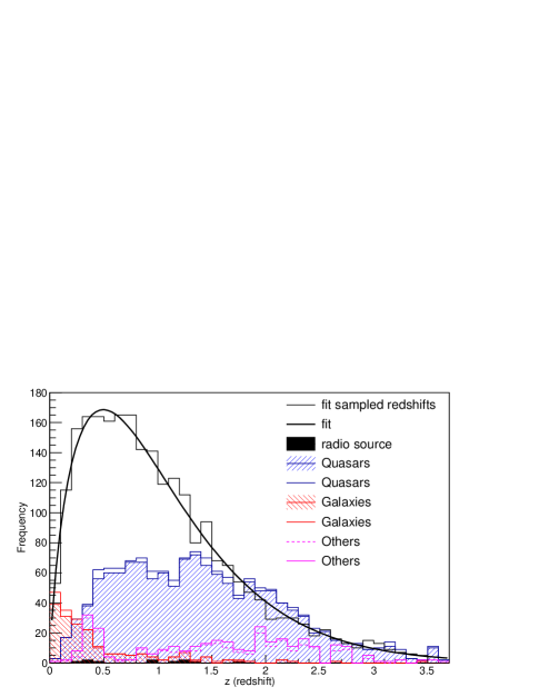
Figure 1: The redshift distributions of different classes of JVAS/CLASS objects. A total of 1921 sources out of 4400 are retrieved from the NED database. The filled (or dashed line) histogram corresponds to NED object match within $0.1$ arcsec, whereas the empty (or solid line) corresponds to NED object match within $0.5$ arcsec. Assuming that the remaining 2479 sources follow radio source redshift number density profile, we have shown one sample input to our simulations.

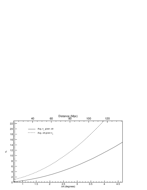
Figure 2: The average angular separation for a fixed number of nearest neighbours ($n_{v}$) and vice versa. Corresponding physical distance scale (Mpc) of the source assuming that it is located at $z=1$ is also given.

4 Correlation Statistic

In order to quantify the correlations between polarizations at different positions we define two statistics, $S_{D}$ and $S^{\prime}_{D}$. Consider the $n_{v}$ nearest neighbours of a source located at site $k$. Let $\psi_{i}$ be the PA of the source at the $i^{th}$ site within the $n_{v}$ nearest neighbour set. The dispersion of PAs in the neighbourhood of this site may be characterized by the measure,

$$d_{k}=\frac{1}{n_{v}}\sum_{i=1,i\neq k}^{n_{v}}\cos[2(\psi_{i}+\Delta_{i\rightarrow k})-2\psi_{k})].$$ (8)

Here the factor $\Delta_{i\rightarrow k}$ arises since the polarizations at two different points, labelled as $i$ and $k$, on the celestial sphere have to be correlated after making a parallel transport from $i\rightarrow k$ (Jain et al., 2004) along the geodesic which connects the two positions. The parameter $\psi_{k}$ in this equation is the PA at the site $k$. The measure $d_{k}$ provides an estimate of the dispersion. We point out that a large value of $d_{k}$ implies low dispersion and vice versa. The statistic is defined as (Hutsemékers, 1998; Jain et al., 2004),

$$S_{D}=\frac{1}{n_{s}}\sum_{k=1}^{n_{s}}d_{k},$$ (9)

where $n_{s}$ is the total number of data samples. A strong alignment between polarization vectors implies a large value of $S_{D}$. We point out that the notation used in this work is different from Tiwari & Jain (2013). We have also dropped self correlations ($i=k$) while calculating $d_{k}$ in equation (8). This changes the magnitude of $S_{D}$ significantly for small $n_{v}$ but does not change the alignment significance results. However, as already mentioned above, in this paper we are considering the jackknife errors which are significantly larger than the variance of $S_{D}$ for the case of the random polarization samples, considered in our previous paper (Tiwari & Jain, 2013). This does lead to an appreciable change in the significance of alignment.

Alternatively we define statistic $S^{\prime}_{D}$ where we measure the dispersion over a fixed angular separation ($\Delta\theta$) rather than measuring it over a fix number of nearest neighbours ($n_{v}$). We point out that these two statistic $S_{D}$ and $S^{\prime}_{D}$ will give same result for a spatially uniform source distribution since for a circle of a given radius the nearest number of sources will be same everywhere. Hence, $S_{D}$ can be translated into $S^{\prime}_{D}$ naively. However, the data sample is expected to show some deviation from spatial uniformity and hence we expect small differences in the two measures, $S_{D}$ and $S^{\prime}_{D}$.

5 Procedure

We first determine the statistic $S_{D}$ ( see equation (9)) for the observed linear PAs. The same procedure is repeated for the theoretical PAs, which are assumed to be aligned perpendicular to the background magnetic field. The magnetic field is generated by simulations as explained in Section 2 and we glean out the galaxies according to redshifts details as given in Fig. 1. For sources where we only have probability distribution of number density, we sample over 100 random outputs of redshifts generated from the probability distribution shown in Fig. 1. Finally, we calculate the $2D$ correlation statistics $S_{D}$ and $S^{\prime}_{D}$. The resulting theoretical values of $S_{D}$ are computed for a range of values of the spectral index $n_{B}$. The best fit value of $n_{B}$ is obtained by making a $\chi^{2}$ fit to the observed data.

In order to compute $\chi^{2}$ we need an estimate of the error in the statistic $S_{D}$. We resort to jackknife errors as we do not know the exact errors in polarization measurements. For computing the jackknife errors, we resample the data by eliminating the $i^{{\rm th}}$ source and calculate the correlation statistics $S_{D}(i)$. We repeat this process for all sources and calculate the $S_{D}(i)$ for $i=1$ to $4213$. We call the full sample statistics as $S_{D}$ and the jackknife error in its estimation is given as

$$(\delta S_{D})^{2}=\frac{(N-1)}{N}\sum^{N}_{i=1}(S_{D}(i)-S_{D})^{2},$$ (10)

where $N$ is the total number of data point, which is 4213 in our case. We add that the jackknife errors do not include systematic errors. The distribution of jackknife sampled $S_{D}$ and a Gaussian fit for $n_{v}=10$ is shown in Fig. 3. Note that the mean of jackknife sampled statistics is almost the same as the full sample $S_{D}$ and so the standard deviation in Fig. 3 is roughly equal to $\delta S_{D}/\sqrt{(N-1)}$. The $\delta S_{D}$ for $n_{v}=10$ as estimated from equation (10) is found to be $0.007716$. We similarly calculate the jackknife errors for all $n_{v}$ and angular scales $\Delta\theta$ for statistics $S_{D}$ and $S^{\prime}_{D}$. In Fig. 4 and 5 the jackknife errors are shown in lowest panel.

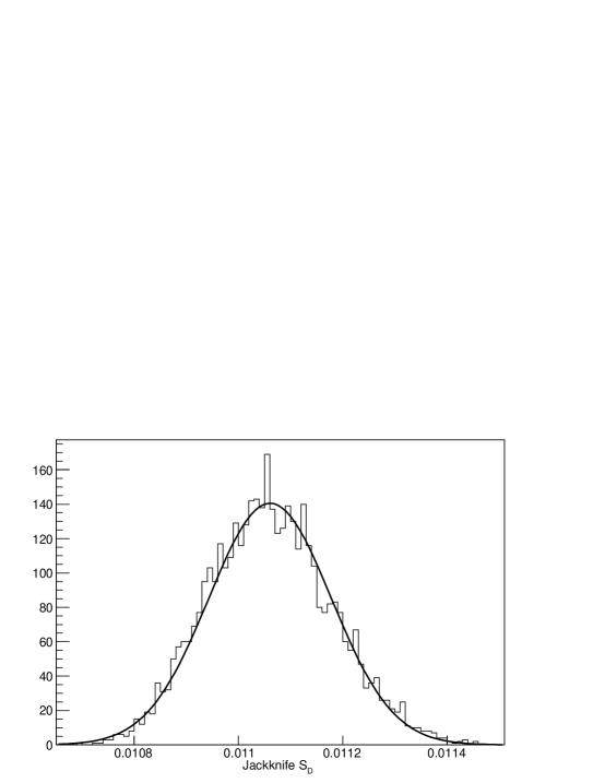
Figure 3: The distribution of jackknife sampled statistics $S_{D}$ for $n_{v}=10$. A fit to Gaussian is also shown. Note that the full sample statistics $S_{D}=0.01106$ is almost equal to the jackknife sampled statistics $S_{D}$ distribution mean ($0.01106$) and so the standard deviation in figure is roughly the $\delta S_{D}/\sqrt{(N-1)}$.

Figure 4: The statistic $S_{D}$ for data with jackknife error bars along with $S_{D}$ corresponding to randomly generated PAs (open circles) are shown in the top panel. The alignment significance considering jackknife errors is plotted in middle panel. For clarity we have plotted jackknife errors $\delta S_{D}$ for each $n_{v}$ in bottom panel.

Figure 5: The statistics $S^{\prime}_{D}$. Data with jackknife error bars along with $S^{\prime}_{D}$ corresponding to random PAs (open circles) are shown in the top panel. The alignment significance considering jackknife errors is plotted in middle panel. The jackknife errors $\delta S^{\prime}_{D}$ are in bottom panel.

6 Results

We simulate the $3D$ magnetic field for $n_{B}$ values in range $-2.20$ to $-2.98$, considering the power law spectrum as discussed in Section 2. As described in Section 3, we have redshifts of 1921 sources and for the remaining sources the redshift is generated assuming a fit obtained in Nusser & Tiwari (2015). We glean out the source location magnetic field directions from simulated magnetic field and calculate the model statistic $S_{D}$. We average over 100 realization to sample over fit generated random redshift positions. The data statistic $S_{D}$ along with alignment significance and jackknife errors is shown in Fig. 4. The model $S_{D}$ values for different $n_{B}$ are fitted with observed data $S_{D}$. The resulting $\chi^{2}$ is defined as

$$\chi^{2}=\sum_{n_{v}=1}^{15}\left(\frac{S_{D}(\rm{observed})-S_{D}(\rm{simulated})}{\delta S_{D}}\right)^{2},$$ (11)

where $\delta S_{D}$ is the jackknife estimate of error in $S_{D}(\rm{observed})$ (see Fig. 4 and 5). We similarly calculate $\chi^{2}$ for $S^{\prime}_{D}$. The maximum value of $n_{v}$ is set equal to 15. This choice is made since the significance of alignment beyond $n_{v}=15$ is within 1-$\sigma$. With one parameter the number of degrees of freedom (DOF) is equal to $14$. We present the $\chi^{2}/DOF$ values verses spectral index $n_{B}$ for statistic $S_{D}$ in Fig. 6. The minimum value of $\chi^{2}/DOF$ is found to be approximately $0.25$ at $n_{B}=-2.76$. The data and best fitted simulated $S_{D}$ comparison for spectral index $n_{B}=-2.76$ is given in Fig. 7. Including one sigma error, the extracted value of $n_{B}$ is found to be, $n_{B}=-2.76\pm 0.04$. We point out that the relatively low value of $\chi^{2}$ indicates that the jackknife errors are large. Nevertheless, even with such large errors we are able to clearly resolve the magnetic field spectral index as seen in Fig. 6.

The results for the case of the alternate statistic $S^{\prime}_{D}$ are also shown in Fig. 6. In this case we set the maximum value of the fixed angular distance $\Delta\theta$ such as to include $15$ nearest neighbour as an average. This corresponds to $\Delta\theta=4.4^{\rm o}$. The full alignment results for statistic $S^{\prime}_{D}$ are shown in Fig. 5. The angular distance corresponding to a mean value of $n_{v}$ is somewhat higher that the average distance for a fixed value of $n_{v}$. We have shown this difference in Fig. 2. Despite this difference, we obtain almost similar results for statistics $S^{\prime}_{D}$. The best fit value of the spectral index is found to be $n_{B}=-2.74\pm 0.04$ (Fig. 6). The slight difference in the extracted values of $n_{B}$ for the two statistics reflects the spatial non-uniformity of data. The value extracted using the statistic $S^{\prime}_{D}$ may be more reliable since it includes sources within a fixed distance from a particular source rather than including a fixed number of nearest neighbours. The $\chi^{2}/DOF$ is slightly lower for $S^{\prime}_{D}$ but the data points at low angular separation ($\Delta\theta<2^{\circ}$) show large fluctuation due to spatial non-uniformity of data. Nevertheless, the results from $S_{D}$ and $S^{\prime}_{D}$ agree within errors. It is interesting that the extracted value of $n_{B}$ is in good agreement with that obtained by magneto-hydrodynamic simulations which suggest a spectral index of $-2.7$ (Dolag et al., 2002). The close agreement may be fortuitous but may be tested by future more refined data. In any case, theoretically, we do not expect a perfect agreement between these two indices. The polarization index ($n_{B}$), extracted from observations, only acts as a tracer of cluster magnetic field index ($n^{\prime}_{B}$). If we assume that the correlations in polarization are induced by those in the cluster magnetic field, we expect that the maximum level of alignment in the polarization orientations would be equal to those of the background magnetic field. The level of alignment, i.e. the value of the statistic $S_{D}$ or $S^{\prime}_{D}$, increases with $|n_{B}|$. Hence we expect that $|n_{B}|\leq|n^{\prime}_{B}|$.

We also point out that since the best fit value of the spectral index is close to the theoretical expectations, we could not have expected a higher significance of alignment in this data set. If we compute the significance using the variance of alignment statistics of shuffled PAs (Tiwari & Jain, 2013), it is found to be about 3 sigmas. However if we include the jackknife errors, the significance is at best about 1.5 sigmas, as shown in Figs. 4 and 5. In order to increase it to 3 sigmas we need to reduce the errors by a factor of two which requires four times more data. Hence a clear test of our proposal can be made by acquiring a suitably enhanced data set.

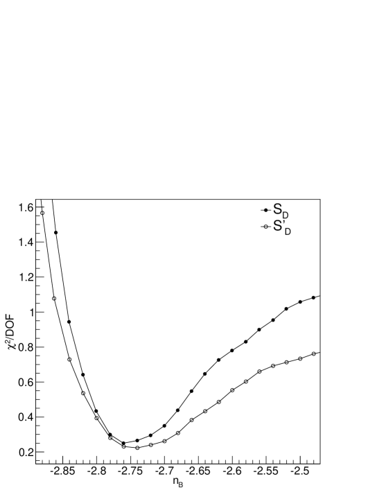
Figure 6: The $\chi^{2}/DOF$ as a function of the spectral index $n_{B}$ for the statistics $S_{D}$ and $S^{\prime}_{D}$.

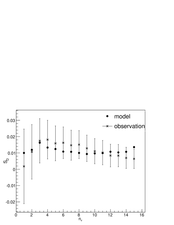
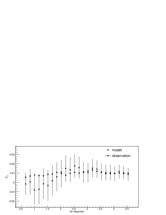
Figure 7: The statistic $S_{D}$ (upper curve) and $S^{\prime}_{D}$ (lower curve) for the real data and simulated polarization from the background magnetic field at the source. This is for the best fitted spectral index $n_{B}=-2.76$ and $n_{B}=-2.74$ respectively.

7 Conclusion and Discussion

We have presented a possible model to explain the large scale radio polarization correlations. The model is based on two main assumptions that the galaxy jets are aligned with cluster magnetic field and that the jet orientations approximately mark the radio polarization angles. We argue that the second assumption is well supported by data and the cosmological magneto-hydrodynamic simulations provide some support for the first assumption. We also find that our extracted value of the spectral index ($n_{B}=-2.74\pm 0.04$) is in good agreement with the value $-2.7$ obtained by magneto-hydrodynamic simulations. This is rather encouraging and provides additional support to our proposal. However given the inherent uncertainties in the polarization data, we cannot claim this to be definitive evidence for our model, which requires further testing with more refined data. We conclude that the observed alignment in the JVAS/CLASS data can be successfully explained in terms of magnetic field correlations. The model can be further applied to other data sets and tested.

References

- Agarwal et al. (2012) Agarwal N., Aluri P. K., Jain P., Khanna U., Tiwari P., 2012, Euro. Phys. Jour. C, 72, 15
- Anderson et al. (2014) Anderson L., Aubourg E., Bailey S., Beutler F., Bhardwaj V., Blanton M., Bolton A. S., Brinkmann J., Brownstein J. R., Burden A., Chuang C.-H., Cuesta A. J., Dawson K. S., et al., 2014, MNRAS, 441, 24
- Best et al. (2003) Best P. N., Arts J. N., Röttgering H. J. A., Rengelink R., Brookes M. H., Wall J., 2003, MNRAS, 346, 627
- De Angelis et al. (2008) De Angelis A., Persic M., Roncadelli M., 2008, Mod. Phys. Lett., A23, 315
- Dolag et al. (2002) Dolag K., Bartelmann M., Lesch H., 2002, A&A, 387, 383
- Eisenstein et al. (2005) Eisenstein D. J., Zehavi I., Hogg D. W., et al., 2005, ApJ, 633, 560
- Gabuzda et al. (1994) Gabuzda D. C., Mullan C. M., Cawthorne T. V., Wardle J. F. C., Roberts D. H., 1994, ApJ, 435, 140
- Helmboldt et al. (2007) Helmboldt J. F., Taylor G. B., Tremblay S., Fassnacht C. D., Walker R. C., Myers S. T., Sjouwerman L. O., Pearson T. J., Readhead A. C. S., Weintraub L., Gehrels N., Romani R. W., Healey S., Michelson P. F., Blandford R. D., Cotter G., 2007, ApJ, 658, 203
- Hutsemékers (1998) Hutsemékers D., 1998, A&A, 332, 410
- Jackson et al. (2007) Jackson N., Battye R., Browne I., Joshi S., Muxlow T., et al., 2007, MNRAS, 376, 371
- Jain et al. (2004) Jain P., Narain G., Sarala S., 2004, MNRAS, 347, 394
- Jedamzik et al. (1998) Jedamzik K., Katalinic V., Olinto A. V., 1998, Phys. Rev., D57, 3264
- Joshi et al. (2007) Joshi S., Battye R., Browne I., Jackson N., Muxlow T., et al., 2007, MNRAS, 380, 162
- Kiessling et al. (2015) Kiessling A., Cacciato M., Joachimi B., Kirk D., Kitching T. D., Leonard A., Mandelbaum R., Schäfer B. M., Sifón C., Brown M. L., Rassat A., 2015, Space Science Reviews, 193, 67
- Kirk et al. (2015) Kirk D., Brown M. L., Hoekstra H., Joachimi B., Kitching T. D., Mandelbaum R., Sifón C., Cacciato M., Choi A., Kiessling A., Leonard A., Rassat A., Schäfer B. M., 2015, Space Science Reviews, 193, 139
- Lister & Smith (2000) Lister M. L., Smith P. S., 2000, ApJ, 541, 66
- Nusser & Tiwari (2015) Nusser A., Tiwari P., 2015, ApJ, 812, 85
- Pelgrims & Hutsemékers (2015) Pelgrims V., Hutsemékers D., 2015, arXiv:1503.03482
- Pollack et al. (2002) Pollack L. K., Taylor G. B., Zavala R. T., 2002, in American Astronomical Society Meeting Abstracts Vol. 34 of Bulletin of the American Astronomical Society, VLBI Polarimetry of 177 Compact, Flat-Spectrum Sources. p. 1182
- Rigby et al. (2011) Rigby E. E., Best P. N., Brookes M. H., Peacock J. a., Dunlop J. S., Röttgering H. J. a., Wall J. V., Ker L., 2011, MNRAS, 416, 1900
- Seshadri & Subramanian (2005) Seshadri T. R., Subramanian K., 2005, Phys. Rev., D72, 023004
- Seshadri & Subramanian (2009) Seshadri T. R., Subramanian K., 2009, Phys. Rev. Lett., 103, 081303
- Shurtleff (2014) Shurtleff R., 2014, arXiv:1408.2514
- Subramanian & Barrow (1998) Subramanian K., Barrow J. D., 1998, Phys. Rev., D58, 083502
- Subramanian et al. (2003) Subramanian K., Seshadri T. R., Barrow J. D., 2003, MNRAS, 344, L31
- Tiwari & Jain (2013) Tiwari P., Jain P., 2013, Int. J. Mod. Phys., D22, 1350089
- Tiwari & Nusser (2015) Tiwari P., Nusser A., 2015, arXiv:1509.02532
- Waddington et al. (2001) Waddington I., Dunlop J. S., Peacock J. A., Windhorst R. A., 2001, MNRAS, 328, 882
- Waddington et al. (2000) Waddington I., Windhorst R. A., Dunlop J. S., Koo D. C., Peacock J. A., 2000, MNRAS, 317, 801
- Weinberg (2008) Weinberg S., 2008, Cosmology. Oxford University Press
- Yamazaki et al. (2010) Yamazaki D. G., Ichiki K., Kajino T., Mathews G. J., 2010, Phys. Rev., D81, 023008