The star-triangle relation and
$3d$ superconformal indices

Abstract.

Superconformal indices of $3d$ $\mathcal{N}=2$ supersymmetric field theories are investigated from the Yang-Baxter equation point of view. Solutions of the star-triangle relation, vertex and IRF Yang-Baxter equations are expressed in terms of the $q$-special functions associated with these $3d$ indices. For a two-dimensional monopole-spin system on the square lattice a free energy per spin is explicitly determined. Similar to the partition functions, superconformal indices of $3d$ theories with the chiral symmetry breaking reduce to Dirac delta functions with the support on chemical potentials of the preserved flavor groups.

1. Introduction

Special functions [2] are key mathematical objects in solvable models of physical phenomena. Quantum integrable systems and related Yang-Baxter equations and quantum algebras [3, 23, 31, 55] have been investigated for a long time in relation to plain hypergeometric functions, their $q$-analogues and elliptic functions. Fairly recently the third class of transcendental functions of hypergeometric type called elliptic hypergeometric integrals has been discovered [48], which strongly extended the database of classical special functions. The cornerstone of the latter functions is the following elliptic beta integral

Theorem (Spiridonov [45]). Let $t_{1},\dots,t_{6},p,q\in{\mathbb{C}}$ with $|t_{1}|,\dots,|t_{6}|,|p|,|q|<1$ and $\prod_{j=1}^{6}t_{j}=pq$. Then

$$\frac{(p;p)_{\infty}(q;q)_{\infty}}{2}\int_{\mathbb{T}}\frac{\prod_{i=1}^{6}\Gamma(t_{i}z^{\pm 1};p,q)}{\Gamma(z^{\pm 2};p,q)}\frac{dz}{2\pi\textup{i}z}=\prod_{1\leq i<j\leq 6}\Gamma(t_{i}t_{j};p,q),$$ (1.1)

where $\Gamma(z;p,q)=(pqz^{-1};p,q)_{\infty}/(z;p,q)_{\infty}$, $(z;p,q)_{\infty}=\prod_{j,k=0}^{\infty}(1-zp^{j}q^{k})$, is the elliptic gamma function and $\mathbb{T}$ is the unit circle of positive orientation.

The first physical application of elliptic hypergeometric integrals consisted in the interpretation of some of them as wave functions or normalizations of wave functions in particular quantum mechanical problems [48]. The most important known application of identity (1.1) was found in [20] in the context of ${\mathcal{N}}=1$ supersymmetric field theories within which it has the meaning of the equality of superconformal indices [36, 40, 41] in Seiberg dual theories [43, 44]. Indeed, the integral on the left-hand side of the equality (1.1) is the superconformal index of the $4d$ ${\mathcal{N}}=1$ supersymmetric gauge theory with $SU(2)$ gauge group and $N_{F}=6$ flavors, chiral scalar multiplets in the fundamental representation of the flavor group $SU(6)$, while the expression on the right side is the superconformal index for the dual theory without gauge degrees of freedom and the chiral fields in the 15-dimensional totally antisymmetric tensor representation of the same flavor group. In other words, the elliptic beta integral is the manifestation of the $s$-confinement phenomenon in gauge theories [43]. The superconformal indices techniques is the most convenient tool for searching new Seiberg dualities [50, 51, 52]. Using properties of the elliptic hypergeometric integrals one can describe uniformly the ’t Hooft anomaly matching conditions [53] and the chiral symmetry breaking [54]. A direct consequence of formula (1.1) was used in topological field theories as well [39].

Another application of relation (1.1) has lead to important progress in the study of exactly solvable models of statistical mechanics. Namely, it has been shown to yield new solutions of the star-triangle relations either in functional [8] or operator forms [16]. Actually, the latter form of the star-triangle relation has been found long before as the integral Bailey lemma [47]. Using the results of [8], a correspondence between the quiver gauge theories and integrable lattice models such that the integrability emerges as a manifestation of the Seiberg type dualities has been established in [49].

Degenerations of the $2d$ spin system of [8] lead to many known models. For instance, the Faddeev-Volkov model [57, 7] or its extension [49] can be obtained in this context as follows. One can reduce superconformal indices of $4d$ theories to the partition functions of $3d$ ${\mathcal{N}}=2$ theories [21]. This reduction leads to the equality of partition functions on the squashed sphere [29] of dual theories expressed in terms of the hyperbolic hypergeometric integral identities.

The star-triangle relation represents a particular form of the Yang-Baxter equations (YBE) standing behind the quantum integrable systems. Another form is the vertex type YBE associated with the integrable spin chains. A powerful techniques for solving such type of equations was developed in [14, 15]. The elliptic beta integral (1.1) and related Bailey lemma [47] played a prominent role in building the most complicated known integral operator solutions of the YBE [16]. In particular, this approach has lead to a new rich class of finite-dimensional solutions of the YBE [11].

In this paper, we present a new solution of the star-triangle relation and other forms of YBE in terms of the basic hypergeometric identity presented in [42]. We relate the Yang-Baxter equations to three-dimensional supersymmetric dualities. The new solution corresponds to the generalized superconformal index of certain $3d$ ${\mathcal{N}}=2$ superconformal gauge theory having a distinguished form due to the contribution of monopoles [30, 32, 35, 37]. Detailed presentation of this correspondence is given in the last section.

2. Notation and definitions

For $q,z\in\mathbb{C}$, $|q|<1,$ we define the infinite $q$-product

$$(z;q)_{\infty}\ :=\ \prod_{k=0}^{\infty}(1-zq^{k}).$$ (2.1)

The (normalized) $q$-gamma function of Jackson has the form [2]

$$\Gamma(z;q)\ :=\frac{1}{(z;q)_{\infty}}.$$ (2.2)

Denote

$$(a,b;q)_{\infty}:=(a;q)_{\infty}(b;q)_{\infty},\quad(ax^{\pm 1};q)_{\infty}:=(ax;q)_{\infty}(ax^{-1};q)_{\infty}$$ (2.3)

with a similar convention for other generalized gamma functions in (1.1) and other relations below.

We need the following $q$-hypergeometric identity.

Theorem. (Rosengren [42]). Let $a_{1},\ldots,a_{6},q\in\mathbb{C}$ and integers $N_{1},\ldots,N_{6}\in\mathbb{Z}$, satisfy the constraints $|a_{j}|,|q|<1$, and $\prod_{j=1}^{6}a_{j}=q$, $\sum_{j=1}^{6}N_{j}=0$. Then

$$\sum_{m\in\mathbb{Z}}\int_{\mathbb{T}}\prod_{j=1}^{6}\frac{(q^{1+\frac{m}{2}}\frac{1}{a_{j}z},q^{1-\frac{m}{2}}\frac{z}{a_{j}};q)_{\infty}}{(q^{N_{j}+\frac{m}{2}}a_{j}z,q^{N_{j}-\frac{m}{2}}\frac{a_{j}}{z};q)_{\infty}}\frac{(1-q^{m}z^{2})(1-q^{m}z^{-2})}{q^{m}z^{6m}}\frac{dz}{2\pi iz}$$

$$\qquad=\frac{2}{\prod_{j=1}^{6}q^{\binom{N_{j}}{2}}a_{j}^{N_{j}}}\prod_{1\leq j<k\leq 6}\frac{(qa_{j}^{-1}a_{k}^{-1};q)_{\infty}}{(q^{N_{j}+N_{k}}a_{j}a_{k};q)_{\infty}},$$ (2.4)

where $\mathbb{T}$ is the unit circle of positive orientation.

This is a $q$-beta sum-integral associated with $3d$ superconformal indices. The proof of the theorem is presented in [27].

Let us define the following generalized $q$-gamma function as a combination of four $q$-gamma functions and $z^{m}$ and $a^{m}$:

$$\Gamma_{q}(a,n;z,m):=\frac{(q^{1+\frac{n+m}{2}}\frac{1}{az},q^{1+\frac{n-m}{2}}\frac{z}{a};q)_{\infty}}{a^{n}z^{m}(q^{\frac{n+m}{2}}az,q^{\frac{n-m}{2}}\frac{a}{z};q)_{\infty}},$$ (2.5)

where $a,z\in\mathbb{C}$ and $n,m\in\mathbb{Z}$.

Lemma. One has the following inversion relation:

$$\Gamma_{q}(a,n;z,m)\Gamma_{q}(b,-n;z,m)=1,\quad ab=q.$$ (2.6)

Proof. Consider the explicit form of the indicated product of $\Gamma_{q}$-functions after the substitution $b=q/a$:

$$\Gamma_{q}(a,n;z,m)\Gamma_{q}({\textstyle\frac{q}{a}},-n;z,m)$$

$$\makebox[40.00006pt]{}=\frac{q^{n}}{z^{2m}a^{2n}}\frac{(q^{1+\frac{n+m}{2}}\frac{1}{az},q^{1+\frac{n-m}{2}}\frac{z}{a},q^{\frac{-n+m}{2}}\frac{a}{z},q^{\frac{-n-m}{2}}az;q)_{\infty}}{(q^{\frac{n+m}{2}}az,q^{\frac{n-m}{2}}\frac{a}{z},q^{1+\frac{-n+m}{2}}\frac{z}{a},q^{1+\frac{-n-m}{2}}\frac{1}{az};q)_{\infty}}.$$ (2.7)

Using the relation $(a;q)_{\infty}=(1-a)(aq;q)_{\infty}$, for $n>m>0$ we can rewrite this expression as

$$\frac{q^{n}}{z^{2m}a^{2n}}\prod_{i=0}^{n+m-1}\frac{1-azq^{i-(m+n)/2}}{1-a^{-1}z^{-1}q^{i+1-(m+n)/2}}\prod_{j=0}^{n-m-1}\frac{1-a^{-1}zq^{i+1+(n-m)/2}}{1-az^{-1}q^{i+(n-m)/2}}=1.$$ (2.8)

For other possible values of the integers $n$ and $m$ one gets the same result due to the properties of $q$-Pochhammer symbols.

Now we can rewrite the above $q$-beta sum-integral in the following compact form.

$$\sum_{m\in\mathbb{Z}}\int_{\mathbb{T}}\prod_{j=1}^{6}\Gamma_{q}(a_{j},n_{j};z,m)[d_{m}z]=\frac{1}{\prod_{j=1}^{6}a_{j}^{2n_{j}}}\prod_{1\leq j<k\leq 6}\frac{(q^{1+\frac{n_{j}+n_{k}}{2}}a_{j}^{-1}a_{k}^{-1};q)_{\infty}}{(q^{\frac{n_{j}+n_{k}}{2}}a_{j}a_{k};q)_{\infty}},$$ (2.9)

where $\prod_{j=1}^{6}a_{j}=q$, $\sum_{j=1}^{6}n_{j}=0$, and

$$[d_{m}z]:=\frac{(1-q^{m}z^{2})(1-q^{m}z^{-2})}{q^{m}}\frac{dz}{4\pi iz},\qquad[d_{m}z]=[d_{-m}z].$$

3. Bailey lemma and the star-triangle relation

Let us define the $D$-function

$$D(t;a,n;z,m):=\Gamma_{q}(q^{\frac{1}{2}}t^{-1}a,n;z,m)\Gamma_{q}(q^{\frac{1}{2}}t^{-1}a^{-1},-n;z,m).$$ (3.1)

It is easy to see that

$$D(t^{-1};a,n;z,m)=\frac{1}{D(t;a,n;z,m)},\qquad D(1;a,n;z,m)=1.$$ (3.2)

Introduce the integral-sum operator of the form

$$M(t)_{x,n;z,m}f_{m}(z):=\frac{(t^{2};q)}{(qt^{-2};q)}\;\sum_{m\in\mathbb{Z}}\int_{\mathbb{T}}[d_{m}z]\;\Gamma_{q}(tx^{\pm 1},\pm n;z,m)f_{m}(z),$$ (3.3)

where

$$\Gamma_{q}(tx^{\pm 1},\pm n;z,m): =\Gamma_{q}(tx,n;z,m)\Gamma_{q}(tx^{-1},-n;z,m)$$

$$=D(q^{1/2}t^{-1};x,n;z,m)$$ (3.4)

and $f_{m}(z)$ is an arbitrary sequence of holomorphic functions.

We note that the following permutational symmetries hold true

$$\Gamma_{q}(tx^{\pm 1},\pm n;z,m)=\Gamma_{q}(tz^{\pm 1},\pm m;x,n),$$ (3.5)

$$D(t;a,n;z,m)=D(t;z,m;a,n).$$ (3.6)

Following the original integral generalization [47, 48] of the Bailey chains techniques [2], we introduce the notion of Bailey pairs in the present context.

Definition. We say that two sequences of functions $\alpha_{m}(z;t)$ and $\beta_{m}(z;t)$, $m\in\mathbb{Z}$, of complex variables $z$ and $t$ form a Bailey pair with respect to the parameter $t$ if they are related by the integral-sum transform (3.3),

$$\beta_{n}(x;t)=M(t)_{x,n;z,m}\alpha_{m}(z;t).$$ (3.7)

Here we assume that $|tx|,|t/x|<1$ and other regions of parameters are reached by the analytical continuation.

Bailey lemma. Suppose we have a particular Bailey pair $\alpha_{k}(x;t),\beta_{k}(x;t)$ with respect to the parameter $t$. Then the sequences of functions

$$\alpha^{\prime}_{k}(x;st)=D(s;y,l;x,k)\alpha_{k}(x;t),$$ (3.8)

$$\beta^{\prime}_{k}(x;st)=D(t^{-1};y,l;x,k)M(s)_{x,k;z,m}D(st;y,l;z,m)\beta_{m}(z;t),$$ (3.9)

where $s,y\in\mathbb{C},l\in\mathbb{Z}$ are arbitrary new parameters, form a Bailey pair with respect to the parameter $st$.

Proof. Let us substitute primed sequences into the relation

$$\beta_{k}^{\prime}(w;st)=M(st)_{w,k;x,j}\alpha_{j}^{\prime}(x;st)$$ (3.10)

and use the inversion $D(t^{-1};y,l;x,k)=1/D(t;y,l;x,k)$. This yields the operator identity

$$M(s)_{w,k;z,m}\;D(st;y,l;z,m)M(t)_{z,m;x,j}=D(t;y,l;w,k)M(st)_{w,k;x,j}D(s;y,l;x,j)$$ (3.11)

known as the star-triangle relation. It is a straightforward consequence of the Rosengren $q$-beta sum-integral. First we compute the expression on the left-hand side of (3.11)

$$\makebox[-20.00003pt]{}\frac{(s^{2},t^{2};q)}{(qs^{-2},qt^{-2};q)}\sum_{m\in\mathbb{Z}}\int_{\mathbb{T}}[d_{m}z]\;\Gamma_{q}(sw^{\pm 1},\pm k;z,m)\Gamma_{q}(q^{\frac{1}{2}}(st)^{-1}y^{\pm 1},\pm l;z,m)$$

$$\makebox[-20.00003pt]{}\times\sum_{j\in\mathbb{Z}}\int_{\mathbb{T}}[d_{j}x]\times\Gamma_{q}(tz^{\pm 1},\pm m;x,j)$$

$$\makebox[-20.00003pt]{}=\frac{(s^{2},t^{2};q)}{(qs^{-2},qt^{-2};q)}\sum_{j\in\mathbb{Z}}\int_{\mathbb{T}}[d_{j}x]\sum_{m\in\mathbb{Z}}\int_{\mathbb{T}}\prod_{j=1}^{6}\Gamma_{q}(a_{j},n_{j};z,m)[d_{m}z],$$ (3.12)

where we used the permutational symmetry of $\Gamma_{q}$-function and have denoted

$$a_{1}=sw,\quad n_{1}=k,\quad a_{2}=\frac{s}{w},\quad n_{2}=-k,\quad a_{3}=\frac{q^{1/2}y}{st},\quad n_{3}=l,\;$$

$$a_{4}=\frac{q^{1/2}}{sty},\quad n_{4}=-l,\quad a_{5}=tx,\quad n_{5}=j,\quad a_{6}=\frac{t}{x},\quad n_{6}=-j.$$ (3.13)

The balancing condition holds true $\prod_{j=1}^{6}a_{j}=q$, $\sum_{j=1}^{6}n_{j}=0$, and we can apply the above formula (2.9) for computing the integral over measure $[d_{m}z]$. This yields the expression

$$\makebox[20.00003pt]{}\frac{(q^{\frac{1+k+l}{2}}\frac{t}{wy},q^{\frac{1+k-l}{2}}\frac{ty}{w},q^{\frac{1-k+l}{2}}\frac{tw}{y},q^{\frac{1-k-l}{2}}twy;q)}{w^{2k}y^{2l}(q^{\frac{1+k+l}{2}}\frac{wy}{t},q^{\frac{1+k-l}{2}}\frac{w}{ty},q^{\frac{1-k+l}{2}}\frac{y}{tw},q^{\frac{1-k-l}{2}}\frac{1}{twy};q)}$$

$$\makebox[-20.00003pt]{}\times\frac{(s^{2}t^{2};q)}{(qs^{-2}t^{-2};q)}\sum_{j\in\mathbb{Z}}\int_{\mathbb{T}}[d_{j}x]\frac{(q^{1+\frac{k+j}{2}}\frac{1}{stwx},q^{1+\frac{k-j}{2}}\frac{x}{stw},q^{1+\frac{-k+j}{2}}\frac{w}{stx},q^{1-\frac{k+j}{2}}\frac{wx}{st};q)}{w^{2k}x^{2j}(q^{\frac{k+j}{2}}stwx,q^{\frac{k-j}{2}}\frac{stw}{x},q^{\frac{-k+j}{2}}\frac{stx}{w},q^{-\frac{k+j}{2}}\frac{st}{wx};q)}$$

$$\makebox[20.00003pt]{}\times\frac{(q^{\frac{1+l+j}{2}}\frac{s}{yx},q^{\frac{1+l-j}{2}}\frac{sx}{y},q^{\frac{1-l+j}{2}}\frac{sy}{x},q^{\frac{1-l-j}{2}}syx;q)}{y^{2l}x^{2j}(q^{\frac{1+l+j}{2}}\frac{yx}{s},q^{\frac{1+l-j}{2}}\frac{y}{sx},q^{\frac{1-l+j}{2}}\frac{x}{sy},q^{\frac{1-l-j}{2}}\frac{1}{syx};q)}$$

$$\makebox[40.00006pt]{}=D(t;y,l;w,k)M(st)_{w,k;x,j}D(s;y,l;x,j),$$ (3.14)

which proves the required identity.

We note that the derived solution of the star-triangle relation resembles structurally a different solution obtained in [33]. We stress that the parameters $y$ and $l$ are dummy variables in this construction, i.e. at each step of the walk along the lattice of Bailey pairs one can introduce further new parameters $y,l\to y^{\prime},l^{\prime}\to\ldots$.

4. Coxeter relations and the vertex type Yang-Baxter equation

Consider elementary transposition operators $s_{j},\,j=1,\ldots,5,$ acting on six parameters $\mathbf{t}=(t_{1},\ldots,t_{6})$:

$$s_{j}(\ldots,t_{j},t_{j+1},\ldots)=(\ldots,t_{j+1},t_{j},\ldots).$$ (4.1)

They generate the permutation group $\mathfrak{S}_{6}$ characterized by the Coxeter relations

$$s_{j}^{2}=1,\quad s_{i}s_{j}=s_{j}s_{i}\ \text{ for }\ |i-j|>1,\quad s_{j}s_{j+1}s_{j}=s_{j+1}s_{j}s_{j+1}.$$ (4.2)

Define now five operators $\mathrm{S}_{j}(\mathbf{t}),\,j=1,\ldots,5,$ acting on the three-index functions of three complex variables $f_{n_{1},n_{2},n_{3}}(z_{1},z_{2},z_{3})$:

$$[\mathrm{S}_{1}(\mathbf{t})f]_{n_{1},n_{2},n_{3}}(z_{1},z_{2},z_{3}):=M(t_{1}/t_{2})_{z_{1},n_{1};z,m}f_{m,n_{2},n_{3}}(z,z_{2},z_{3}),\quad$$

$$[\mathrm{S}_{2}(\mathbf{t})f]_{n_{1},n_{2},n_{3}}(z_{1},z_{2},z_{3}):=D(t_{2}/t_{3};z_{1},n_{1};z_{2},n_{2})f_{n_{1},n_{2},n_{3}}(z_{1},z_{2},z_{3}).$$

$$[\mathrm{S}_{3}(\mathbf{t})f]_{n_{1},n_{2},n_{3}}(z_{1},z_{2},z_{3}):=M(t_{3}/t_{4})_{z_{2},n_{2};z,m}f_{n_{1},m,n_{3}}(z_{1},z,z_{3}),$$

$$[\mathrm{S}_{4}(\mathbf{t})f]_{n_{1},n_{2},n_{3}}(z_{1},z_{2},z_{3}):=D(t_{4}/t_{5};z_{2},n_{2};z_{3},n_{3})f_{n_{1},n_{2},n_{3}}(z_{1},z_{2},z_{3}),$$

$$[\mathrm{S}_{5}(\mathbf{t})f]_{n_{1},n_{2},n_{3}}(z_{1},z_{2},z_{3}):=M(t_{5}/t_{6})_{z_{3},n_{3};z,m}f_{n_{1},n_{2},m}(z_{1},z_{2},z),$$

We stress that all these operators depend on the ratios of parameters, $\mathrm{S}_{j}(\mathbf{t})=\mathrm{S}_{j}(t_{j}/t_{j+1})$. Let us prove that for an appropriate space of test functions the operators $\mathrm{S}_{j}$ generate the group $\mathfrak{S}_{6}$, provided their sequential action is defined via a cocycle condition $\mathrm{S}_{j}\mathrm{S}_{k}:=\mathrm{S}_{j}(s_{k}(\mathbf{t}))\mathrm{S}_{k}(\mathbf{t})$. For this it is necessary to verify the Coxeter relations

$$\mathrm{S}_{j}^{2}=1,\quad\mathrm{S}_{i}\mathrm{S}_{j}=\mathrm{S}_{j}\mathrm{S}_{i}\ \text{ for }\ |i-j|>1,\quad\mathrm{S}_{j}\mathrm{S}_{j+1}\mathrm{S}_{j}=\mathrm{S}_{j+1}\mathrm{S}_{j}\mathrm{S}_{j+1}.$$ (4.3)

Indeed, the latter relations are equivalent to algebraic properties of the Bailey lemma entries, in complete analogy with the elliptic hypergeometric case [16]. It is sufficient to establish them for $\mathrm{S}_{1}$ and $\mathrm{S}_{2}$, others will follow by the symmetry. So, we have

$$\mathrm{S}_{2}^{2}=\mathrm{S}_{2}(s_{2}\mathbf{t})\mathrm{S}_{2}(\mathbf{t})=D(t_{3}/t_{2};z_{1},n_{1};z_{2},n_{2})D(t_{2}/t_{3};z_{1},n_{1};z_{2},n_{2})=1.$$ (4.4)

A substantially more complicated relation is needed for $\mathrm{S}_{1}$:

$$\makebox[-20.00003pt]{}[\mathrm{S}_{1}^{2}f]_{n}(x)=[\mathrm{S}_{1}(s_{1}\mathbf{t})\mathrm{S}_{1}(\mathbf{t})f]_{n}(x)=M(t^{-1})_{x,n;z,m}M(t)_{z,m;y,j}f_{j}(y)$$ (4.5)

$$=\sum_{j\in\mathbb{Z}}\int[d_{j}y]\;f_{j}(y)(1-t^{2})(1-t^{-2})\;$$

$$\qquad\times\sum_{m\in\mathbb{Z}}\int[d_{m}z]\;\Gamma_{q}(t^{-1}x^{\pm 1},\pm n;z,m)\Gamma_{q}(ty^{\pm 1},\pm j;z,m)=f_{n}(x),\quad t=\frac{t_{1}}{t_{2}},$$

or $\mathrm{S}_{1}^{2}=\hbox{{1}\kern-2.5pt\hbox{l}}$. First, we claim that

$$M(1)=\hbox{{1}\kern-2.5pt\hbox{l}},\quad\text{or}\quad M(1)_{z,m;y,j}f_{j}(y)=f_{m}(z)$$

for the holomorphic test functions satisfying the reflection symmetry $f_{-m}(y^{-1})=f_{m}(y)$. This fact follows from the residue calculus. For $t\to 1$ two pairs of poles approach the integration contour in $M(t)_{z,m;y,j}f_{j}(y)$ from two sides and pinch it. To resolve the singularity it is necessary to compute two residues which leads to the expression $(f_{m}(z)+f_{-m}(z^{-1}))/2$, and the reflection symmetry reduces it to one term. We now substitute in the star-triangle relation (3.11) the constraint $st=1$. Using the inversion relation for $D$-function and $D(1;z_{1},n_{1};z_{2},n_{2})=1$, the $D$-terms disappear on both sides and we obtain $M(t^{-1})M(t)=\hbox{{1}\kern-2.5pt\hbox{l}}$.

Finally,

$$\makebox[-20.00003pt]{}\mathrm{S}_{1}\mathrm{S}_{2}\mathrm{S}_{1}=\mathrm{S}_{1}(s_{2}s_{1}\mathbf{t})\mathrm{S}_{2}(s_{1}\mathbf{t})\mathrm{S}_{1}(\mathbf{t})=M(\textstyle{\frac{t_{2}}{t_{3}}})_{z_{1},n_{1};z,m}D(\textstyle{\frac{t_{1}}{t_{3}}};z_{2},n_{2};z,m)M(\textstyle{\frac{t_{1}}{t_{2}}})_{z,m;x,j}$$

$$\makebox[40.00006pt]{}=\mathrm{S}_{2}\mathrm{S}_{1}\mathrm{S}_{2}=\mathrm{S}_{2}(s_{1}s_{2}\mathbf{t})\mathrm{S}_{1}(s_{2}\mathbf{t})\mathrm{S}_{2}(\mathbf{t})$$

$$\makebox[40.00006pt]{}=D(\textstyle{\frac{t_{1}}{t_{2}}};z_{1},n_{1};z_{2},n_{2})M(\textstyle{\frac{t_{1}}{t_{3}}})_{z_{1},n_{1};x,j}D(\textstyle{\frac{t_{2}}{t_{3}}};x,j;z_{2},n_{2}),$$ (4.6)

which is precisely the star-triangle relation.

Consider the tensor product of three infinite-dimensional (equal or different) spaces $\mathbb{V}_{1}\otimes\mathbb{V}_{2}\otimes\mathbb{V}_{3}$ and associate with each space $\mathbb{V}_{j}$ a pair of variables: the spectral parameter $u_{j}$ and the spin variable $g_{j}$, respectively. Define R-operators $\mathbb{R}_{ik}(u_{i},g_{i}|u_{k},g_{k})$ acting in a non-trivial way in the subspace $\mathbb{V}_{i}\otimes\mathbb{V}_{k}$ with the unity operator action in its complement. The vertex type YBE has the form

$$\mathbb{R}_{12}(u_{1},g_{1}|u_{2},g_{2})\,\mathbb{R}_{13}(u_{1},g_{1}|u_{3},g_{3})\,\mathbb{R}_{23}(u_{2},g_{2}|u_{3},g_{3})$$ (4.7)

$$\makebox[30.00005pt]{}=\mathbb{R}_{23}(u_{2},g_{2}|u_{3},g_{3})\,\mathbb{R}_{13}(u_{1},g_{1}|u_{3},g_{3})\,\mathbb{R}_{12}(u_{1},g_{1}|u_{2},g_{2}).$$

Actually, the R-operators depend on the difference of spectral parameters,

$$\mathbb{R}_{ik}(u_{i},g_{i}|u_{k},g_{k})=\mathbb{R}_{ik}(u_{i}-u_{j}),$$ (4.8)

where we omitted dependence on the spin variables. Using this notation we can rewrite YBE in the more conventional form

$$\mathbb{R}_{12}(u-v)\,\mathbb{R}_{13}(u-w)\,\mathbb{R}_{23}(v-w)=\mathbb{R}_{23}(v-w)\,\mathbb{R}_{13}(u-w)\,\mathbb{R}_{12}(u-v),$$ (4.9)

where $u=u_{1},v=u_{2},w=u_{3}$. It is convenient to single out the permutation operators from the R-operator

$$\mathbb{R}_{ik}(u)=\mathbb{P}_{ik}\,\mathrm{R}_{ik}(u),$$ (4.10)

where the operator $\mathbb{P}_{ik}$ interchanges the spaces, $\mathbb{P}_{ik}(\mathbb{V}_{i}\otimes\mathbb{V}_{k})=\mathbb{V}_{k}\otimes\mathbb{V}_{i}$. Removing these permutation operators from the Yang-Baxter equation (4.7) yields the relation

$$\mathrm{R}_{23}(u_{1},g_{1}|u_{2},g_{2})\,\mathrm{R}_{12}(u_{1},g_{1}|u_{3},g_{3})\,\mathrm{R}_{23}(u_{2},g_{2}|u_{3},g_{3})\,$$

$$\makebox[30.00005pt]{}=\mathrm{R}_{12}(u_{2},g_{2}|u_{3},g_{3})\,\mathrm{R}_{23}(u_{1},g_{1}|u_{3},g_{3})\,\mathrm{R}_{12}(u_{1},g_{1}|u_{2},g_{2}),$$ (4.11)

where one sees only two R-operators, $\mathrm{R}_{12}$ and $\mathrm{R}_{23}$.

Let us fix the spaces $\mathbb{V}_{j}$ as copies of the infinite bilateral sequences of meromorphic functions $f_{j}(z),\,j\in\mathbb{Z}$. Then the triple tensor product of interest takes the form $\mathbb{V}_{1}\otimes\mathbb{V}_{2}\otimes\mathbb{V}_{3}=f_{n_{1},n_{2},n_{3}}(z_{1},z_{2},z_{3})$. Define now the composite operators acting in this space $\mathrm{R}_{12}(\mathbf{t})$,

$$\mathrm{R}_{12}(\mathbf{t})=\mathrm{R}_{12}(t_{1},\ldots,t_{4})=\mathrm{S}_{2}(s_{1}s_{3}s_{2}\mathbf{t})\,\mathrm{S}_{1}(s_{3}s_{2}\mathbf{t})\,\mathrm{S}_{3}(s_{2}\mathbf{t})\,\mathrm{S}_{2}(\mathbf{t})$$ (4.12)

$$\makebox[40.00006pt]{}=\mathrm{S}_{2}(t_{1}/t_{4})\mathrm{S}_{1}(t_{1}/t_{3})\mathrm{S}_{3}(t_{2}/t_{4})\,\mathrm{S}_{2}(t_{2}/t_{3}),$$

and $\mathrm{R}_{23}(\mathbf{t})$,

$$\mathrm{R}_{23}(\mathbf{t})=\mathrm{R}_{23}(t_{3},\ldots,t_{6})=\mathrm{S}_{4}(s_{3}s_{5}s_{4}\mathbf{t})\,\mathrm{S}_{3}(s_{5}s_{4}\mathbf{t})\,\mathrm{S}_{5}(s_{4}\mathbf{t})\,\mathrm{S}_{4}(\mathbf{t})$$ (4.13)

$$\makebox[40.00006pt]{}=\mathrm{S}_{4}(t_{3}/t_{6})\,\mathrm{S}_{3}(t_{3}/t_{5})\,\mathrm{S}_{5}(t_{4}/t_{6})\,\mathrm{S}_{4}(t_{4}/t_{5}).$$

Denoting

$$t_{1,2}=e^{-\pi i(u\pm g_{1})},\quad t_{3,4}=e^{-\pi i(v\pm g_{2})},\quad t_{5,6}=e^{-\pi i(w\pm g_{3})},$$ (4.14)

one can identify

$$\mathrm{R}_{12}(\mathbf{t})=\mathrm{R}_{12}(u,g_{1}|v,g_{2}),\qquad\mathrm{R}_{23}(\mathbf{t})=\mathrm{R}_{23}(v,g_{2}|w,g_{3})$$ (4.15)

and check that these operators depend only on the difference of spectral parameters $u-v$ and $v-w$, respectively.

Theorem. The R-operators (4.12) and (4.13) satisfy the vertex type Yang-Baxter relation (4.11).

Proof. Substituting the explicit forms of the R-operators into equality (4.11), we come to the relation

$$\mathrm{S}_{4}\mathrm{S}_{3}\mathrm{S}_{5}\mathrm{S}_{4}\cdot\mathrm{S}_{2}\mathrm{S}_{1}\mathrm{S}_{3}\mathrm{S}_{2}\cdot\mathrm{S}_{4}\mathrm{S}_{3}\mathrm{S}_{5}\mathrm{S}_{4}=\mathrm{S}_{2}\mathrm{S}_{1}\mathrm{S}_{3}\mathrm{S}_{2}\cdot\mathrm{S}_{4}\mathrm{S}_{3}\mathrm{S}_{5}\mathrm{S}_{4}\cdot\mathrm{S}_{2}\mathrm{S}_{1}\mathrm{S}_{3}\mathrm{S}_{2},$$ (4.16)

which is easily checked using only the cubic Coxeter relations for operators $\mathrm{S}_{j}$ in complete analogy with the cases considered in [15, 16].

5. A new two-dimensional solvable lattice model

Let us apply the operator relation (3.11) to a product of the Kronecker and Dirac delta-functions which remove integration over the $x$-variable and summation over the index $j$. This yields the functional star-triangle relation of the form

$$\sum_{m\in\mathbb{Z}}\int_{0}^{1}\rho_{m}(u)\mathrm{W}_{\xi-a}(x,j;u,m)\mathrm{W}_{a+b}(y,j;u,m)\mathrm{W}_{\xi-b}(w,l;u,m)du$$

$$\makebox[20.00003pt]{}=\chi(a,b)\mathrm{W}_{b}(x,j;y,k)\mathrm{W}_{\xi-a-b}(x,j;w,l)\mathrm{W}_{a}(y,k;w,l),$$ (5.1)

where

$$\mathrm{W}_{a}(x,j;u,m)=\Gamma_{q}(e^{2\pi i(a-\xi\pm x\pm u)}),\quad e^{-4\pi\textup{i}\xi}:=q,$$ (5.2)

and

$$\rho_{m}(u) =\frac{(1-q^{m}e^{4\pi iu})(1-q^{m}e^{-4\pi iu})}{2q^{m}},$$ (5.3)

$$\quad\chi(a,b) =\frac{(qe^{4\pi ia},qe^{4\pi ib},e^{-4\pi i(a+b)};q)_{\infty}}{(e^{-4\pi ia},e^{-4\pi ib},qe^{4\pi i(a+b)};q)_{\infty}}.$$ (5.4)

We now define a two-dimensional lattice model associated with this relation. Consider a honeycomb lattice with the spins denoted by labels $x,u,w,$ etc which seat in vertices. Each spin has a discrete internal degree of freedom denoted as $m,j,k,l,$ etc (the monopole number). Neighboring spins $(x,j)$ and $(u,m)$ interact along the edges connecting them with the energy determined by the Boltzmann weight $\mathrm{W}_{a}(x,j;u,m)$. The function $\rho_{m}(u)$ describes the self-energy of spins, and $\xi$ is called the crossing parameter. In this picture the “integration-plus-summation” in the star-triangle relation (5.1) means computation of the partition function for an elementary star-shaped cell with contributions coming from all possible values of the continuous spin $u$ sitting in the central vertex and all possible values of the magnetic charge $m$. The honeycomb lattice can be transformed using the star-triangle relation to triangular and square lattices.

Compose now $N\times M$ sized two-dimensional square lattice of spins and associate with each horizontal edge the weight $\mathrm{W}_{a}(x,j;u,m)$ and with the vertical one the weight $\mathrm{W}_{\xi-a}(x,j;u,m)$. Then the partition function of such homogeneous spin system with the internal spin energy $\rho_{m}(u)$ has the form

$$Z=\sum_{\mathbb{Z}^{NM}}\int_{[0,1]^{NM}}\prod_{(ij)}\mathrm{W}_{a}(u_{i},m_{i};u_{j},m_{j})\prod_{(kl)}\mathrm{W}_{\xi-a}(u_{k},m_{k};u_{l},m_{l})\prod_{s}\rho_{m_{s}}(u_{s})du_{s},$$ (5.5)

where the first product is taken over the horizontal edges $(ij)$, the second product goes over all vertical edges $(k,l)$, and the third product (in $s$) is taken over all internal vertices of the lattice. Then one can consider the thermodynamical limit of infinite lattice, $N,M\to\infty$, and look for the free energy per spin $\kappa(a)$ found from the asymptotics

$$Z(a)\ \mathrel{\mathop{=}\limits_{N,M\to\infty}}e^{-NM\kappa(a)}.$$ (5.6)

Conjecturally, similar to the models considered in [7, 8, 49], the value of $\kappa(a)$ can be found using the reflection method [6]. Namely, one renormalizes the Bolztmann weights

$$\mathrm{\widetilde{W}}_{a}(x,j;u,m)=\frac{1}{m(a)}\mathrm{W}_{a}(x,j;u,m)$$ (5.7)

and chooses the multiplier $m(a)$ in such a way that the star-triangle relation takes the form

$$\sum_{m\in\mathbb{Z}}\int_{0}^{1}\rho_{m}(u)\mathrm{\widetilde{W}}_{\xi-a}(x,j;u,m)\mathrm{\widetilde{W}}_{a+b}(y,j;u,m)\mathrm{\widetilde{W}}_{\xi-b}(w,l;u,m)du$$

$$\makebox[20.00003pt]{}=\mathrm{\widetilde{W}}_{b}(x,j;y,k)\mathrm{\widetilde{W}}_{\xi-a-b}(x,j;w,l)\mathrm{\widetilde{W}}_{a}(y,k;w,l).$$ (5.8)

Then,

$$Z(a)\ \mathrel{\mathop{=}\limits_{N,M\to\infty}}m(a)^{NM},\quad\text{or}\quad\kappa(a)=-\log m(a).$$ (5.9)

Such a transformation of star-triangle relation requires

$$\frac{m(\xi-a)m(\xi-b)m(a+b)}{m(a)m(b)m(\xi-a-b)}=\chi(a,b),$$ (5.10)

which is possible if $m(a)$ satisfies the equation

$$\frac{m(a)}{m(\xi-a)}\frac{(e^{4\pi i(a-\xi)};q)_{\infty}}{(e^{-4\pi ia};q)_{\infty}}=1,\quad\text{or}\quad m(a+\xi)=\frac{(e^{-4\pi i(a+\xi)};q)_{\infty}}{(e^{4\pi ia};q)_{\infty}}m(-a).$$ (5.11)

Introduce the following infinite product

$$f(x;p,q)=(x;p,q)_{\infty}(pqx^{-1};p,q)_{\infty},\qquad\frac{f(px;p,q)}{f(x;p,q)}=\frac{(qx^{-1};q)_{\infty}}{(x;q)_{\infty}}.$$ (5.12)

We note that this is the product of the numerator and denominator of the elliptic gamma function. One has the following inversion relation

$$f(x^{-1};p,q)=f(pqx;p,q).$$ (5.13)

Define the composite function

$$\mu(x;p,q)=\frac{f(xp\sqrt{pq};p^{2},q)}{f(x\sqrt{pq};p^{2},q)}.$$ (5.14)

It satisfies the equations

$$\mu(x;p,q)\mu(x^{-1};p,q)=1,\qquad\mu(x;p,q)\mu(p^{-1}x;p,q)=\frac{(x^{-1}p^{1/2}q^{1/2};q)_{\infty}}{(xp^{-1/2}q^{1/2};q)_{\infty}}.$$ (5.15)

Using these relations we can set

$$m(a)=\mu(e^{4\pi ia};q,q)=\frac{(q^{2}e^{4\pi ia},qe^{-4\pi ia};q,q^{2})_{\infty}}{(qe^{4\pi ia},q^{2}e^{-4\pi ia};q,q^{2})_{\infty}}$$ (5.16)

and see that this function satisfies the unitarity condition

$$m(-a)=\frac{1}{m(a)}$$ (5.17)

and the key starting equation (5.11). So, $-\log m(a)$ provides the explicit expression for the free energy per spin of the discussed two-dimensional “spin” model. For the model with the Boltzmann weights (5.7) the free energy is equal to zero.

6. Star-star relations and an IRF model Boltzmann weight

We consider the simplest consequence of the Bailey chain of identities for sums of $q$-hypergeometric integrals described above following the elliptic hypergeometric pattern [47]. For this we use the evident explicit Bailey pair, following from the integration formula (2.9). Namely, let us choose

$$\alpha_{m}(z,t)=\prod_{j=1}^{4}\Gamma_{q}(a_{j},n_{j};z,m),$$ (6.1)

where $a_{j}$ are arbitrary parameters. Substituting this expression into the integral transformation (3.7), imposing the constraint $\sum_{j=1}^{4}n_{j}=0$, and choosing $t^{2}=q\prod_{j=1}^{4}a_{j}^{-1}$, we derive from the Rosengren identity that

$$\beta_{n}(x;t)=\frac{1}{x^{4n}\prod_{j=1}^{4}a_{j}^{2n_{j}}}\prod_{1\leq j<k\leq 4}\frac{(q^{1+\frac{n_{j}+n_{k}}{2}}a_{j}^{-1}a_{k}^{-1};q)_{\infty}}{(q^{\frac{n_{j}+n_{k}}{2}}a_{j}a_{k};q)_{\infty}}$$

$$\makebox[40.00006pt]{}\times\prod_{j=1}^{4}\frac{(q^{1+\frac{n_{j}+n}{2}}a_{j}^{-1}t^{-1}x^{-1},q^{1+\frac{n_{j}-n}{2}}a_{j}^{-1}t^{-1}x;q)_{\infty}}{(q^{\frac{n_{j}+n}{2}}a_{j}tx,q^{\frac{n_{j}-n}{2}}a_{j}tx^{-1};q)_{\infty}}.$$ (6.2)

We now take definitions of the Bailey lemma entries (3.8) and (3.9) and substitute them into the relation $\beta_{k}^{\prime}(w;st)=M(st)_{w,k;x,j}\alpha_{j}^{\prime}(x;st)$. This yields the following explicit symmetry transformation law

$$V(\underline{a},\underline{n};q)=\frac{V(\underline{\tilde{a}},\underline{n};q)}{\prod_{j=1}^{8}a_{j}^{n_{j}}}\prod_{1\leq j<k\leq 4}\frac{(q^{1+\frac{n_{j}+n_{k}}{2}}a_{j}^{-1}a_{k}^{-1},q^{1+\frac{n_{j+4}+n_{k+4}}{2}}a_{j+4}^{-1}a_{k+4}^{-1};q)_{\infty}}{(q^{\frac{n_{j}+n_{k}}{2}}a_{j}a_{k},q^{\frac{n_{j+4}+n_{k+4}}{2}}a_{j+4}a_{k+4};q)_{\infty}},$$ (6.3)

where

$$V(\underline{a},\underline{n};q):=\sum_{m\in\mathbb{Z}}\int_{\mathbb{T}}\prod_{j=1}^{8}\Gamma_{q}(a_{j},n_{j};z,m)[d_{m}z],\qquad\prod_{j=1}^{8}a_{j}=q^{2},\quad\sum_{j=1}^{8}n_{j}=0$$ (6.4)

and the following notation for the parameters is used

$$a_{5,6}=stw^{\pm 1},\quad n_{5,6}=\pm k,\quad a_{7,8}=q^{1/2}s^{-1}y^{\pm 1},\quad n_{7,8}=\pm l$$ (6.5)

as well as

$$\tilde{a}_{j}=ta_{j},\quad j=1,2,3,4,\qquad\tilde{a}_{j}=t^{-1}a_{j},\quad j=5,6,7,8.$$ (6.6)

Remind also the constraint $t^{2}\prod_{j=1}^{4}a_{j}=q$.

Conjecture. Let us take the $V$-function, whose parameters $a_{j},n_{j}$ satisfy only the balancing conditions indicated in the definition (6.4) and an additional constraint $\sum_{j=1}^{4}n_{j}=0$. Then we conjecture that it satisfies the symmetry transformation (6.3), where

$$\left\{\begin{array}[]{cl}\tilde{a}_{j}=\varepsilon a_{j},&j=1,2,3,4\\ \tilde{a}_{j}=\varepsilon^{-1}t_{j},&j=5,6,7,8\end{array}\right.;\quad\varepsilon=\sqrt{\frac{q}{a_{1}a_{2}a_{3}a_{4}}}=\sqrt{\frac{a_{5}a_{6}a_{7}a_{8}}{q}}.$$ (6.7)

Indeed, using the relation

$$\frac{(q^{1-m/2}z^{-1};q)_{\infty}}{(q^{-m/2}z;q)_{\infty}}=\frac{q^{m/2}}{(-z)^{m}}\frac{(q^{1+m/2}z^{-1};q)_{\infty}}{(q^{+m/2}z;q)_{\infty}},\quad m\in\mathbb{Z},$$ (6.8)

one can verify that a repetition of the transformation (6.3), (6.7) returns back the original $V$-function, i.e. we deal with a reflection. The map $a_{j}\to\tilde{a}_{j}$ is the key reflection extending the Weyl group $S_{8}$ of the root system $A_{7}$ to the Weyl group of the exceptional root system $E_{7}$. However, because of the presence of integers $n_{j}$ and the constraint $\sum_{j=1}^{4}n_{j}=0$ we do not have the full $W(E_{7})$ symmetry of the $V$-function yet. Interestingly, even in this reduced case the Bailey chains techniques yields the symmetry transformation (6.3) only when a pair of integers is forced to take particular values $n_{i}+n_{j}=n_{k}+n_{l}=0$, $i\neq j\neq k\neq l$, which contrasts with the elliptic hypergeometric $V$-function case [46, 48].

Consider a $2d$ checkerboard lattice [4] where each “black” site has four “white” neighbours and, vice versa, each “white” site has four “black” neighbours. Ascribe to each edge connecting the white and black sites the Boltzmann weight $\mathrm{W}_{\alpha_{i}}$ (5.2) with arbitrary parameters $\alpha_{i}$ subject to the constraint $\sum_{j=1}^{4}\alpha_{j}=2\xi$. An IRF model is obtained when we integrate out the one-color lattice spins. The Boltzmann weight of the corresponding elementary “cell” containing four vertices determines the energy of this square face. It is given obviously by a special case of the general $V$-function introduced above when all integer variables $n_{j}$ are paired by the relation $n_{2i-1}+n_{2i}=0$. Then, completely similarly to [49], the symmetry transformation (6.3) has now the interpretation as a star-star relation [4]. As shown by Baxter [5] knowledge of the star-star relations automatically leads to the YBE for IRF models.

7. IRF Yang-Baxter equation with spectral parameter

The Yang-Baxter equation for IRF models (or SOS-type YBE) [12, 13] associated with $3d$ superconformal indices has the following form

$$\sum_{H\in\mathbb{Z}}\int[d_{H}h]\;R_{t_{41}t_{63}}\left(\begin{array}[]{cc}{a,A}&{}{b,B}\\ {}{h,H}&{}{c,C}\end{array}\right)\;R_{t_{63}t_{25}}\left(\begin{array}[]{cc}{}{c,C}&{}{d,D}\\ {}{h,H}&{}{e,E}\end{array}\right)$$ (7.5)

$$\makebox[20.00003pt]{}\times R_{t_{25}t_{41}}\left(\begin{array}[]{cc}{}{e,E}&{}{f,F}\\ {}{h,H}&{}{a,A}\end{array}\right)=\sum_{H\in\mathbb{Z}}\int[d_{H}h]\;R_{t_{63}t_{25}}\left(\begin{array}[]{cc}{}{b,B}&{}{h,H}\\ {}{a,A}&{}{f,F}\end{array}\right)$$ (7.10)

$$\makebox[40.00006pt]{}\times R_{t_{25}t_{41}}\left(\begin{array}[]{cc}{}{d,D}&{}{h,H}\\ {}{c,C}&{}{b,B}\end{array}\right)\;R_{t_{41}t_{25}}\left(\begin{array}[]{cc}{}{f,F}&{}{h,H}\\ {}{e,E}&{}{d,D}\end{array}\right),$$ (7.15)

where we introduced for convenience the shorthand notation for spectral parameters $t_{ij}=(t_{i},t_{j})$. The following statistical weight satisfies this equation

$$R_{(m,l)(n,r)}\left(\begin{array}[]{cc}{}{a,A}&{}{b,B}\\ {}{d,D}&{}{c,C}\end{array}\right) \ =\frac{(q^{\frac{2}{3}}(n/l)^{-2},q^{\frac{2}{3}}(r/m)^{-2};q)_{\infty}}{(q^{\frac{1}{3}}(n/l)^{2},q^{\frac{1}{3}}(r/m)^{2};q)_{\infty}}\sum_{k\in\mathbb{Z}}\int[d_{k}z]$$ (7.18)

$$\times\Gamma_{q}(q^{\frac{1}{3}}\frac{l}{n}a^{\pm 1},\pm A;z,k)\Gamma_{q}(q^{\frac{1}{6}}\frac{r}{l}b^{\pm 1},\pm B;z,k)$$

$$\times\Gamma_{q}(q^{\frac{1}{3}}\frac{m}{r}c^{\pm 1},\pm C;z,k)\Gamma_{q}(q^{\frac{1}{6}}\frac{n}{m}d^{\pm 1},\pm D;z,k).$$ (7.19)

It is substantially equal to the $V$-function (6.4) with particular constraints on the integers $\underline{n}=(\pm A,\pm B,\pm C,\pm D)$.

For showing that function (7.19) describes a solution of equation (7.15) we use a special case of identity (2.9) associated with the star-triangle relation

$$\sum_{m\in\mathbb{Z}}\int[d_{m}z]\Gamma_{q}(q^{\frac{1}{6}}t/sa^{\pm 1},\pm A;z,m)\Gamma_{q}(q^{\frac{1}{6}}s/rb^{\pm 1},\pm B;z,m)\Gamma_{q}(q^{\frac{1}{6}}r/tc^{\pm 1},\pm C;z,m)$$

$$\ =\ \frac{(q^{\frac{2}{3}}(t/s)^{-2},q^{\frac{2}{3}}(s/r)^{-2},q^{\frac{2}{3}}(r/t)^{-2};q)_{\infty}}{(q^{\frac{1}{3}}(t/s)^{2},q^{\frac{1}{3}}(s/r)^{2},q^{\frac{1}{3}}(r/t)^{2};q)_{\infty}}\Gamma_{q}(q^{\frac{1}{3}}t/ra^{\pm 1},\pm A;b,B)$$

$$\qquad\times\;\Gamma_{q}(q^{\frac{1}{3}}r/sc^{\pm 1},\pm C;a,A)\Gamma_{q}(q^{\frac{1}{3}}s/tb^{\pm 1},\pm B;c,C).$$ (7.20)

We now form the following composite function defined by 6 integrations and 6 discrete summations

$$\sum_{m_{i}\in\mathbb{Z}}\int\prod_{i=1}^{6}[d_{m_{i}}z]\;\Gamma_{q}(q^{\frac{1}{6}}t_{1}/t_{5}f^{\pm 1},\pm F;z_{6},m_{6})\Gamma_{q}(q^{\frac{1}{6}}t_{6}/t_{1}z_{6}^{\pm 1},\pm m_{6};z_{1},m_{1})$$

$$\qquad\qquad\times\;\Gamma_{q}(^{\frac{1}{6}}t_{2}/t_{6}a^{\pm 1},\pm A;z_{1},m_{1})\;\Gamma_{q}(q^{\frac{1}{6}}t_{1}/t_{2}z_{2}^{\pm 1},\pm m_{2};z_{1},m_{1})$$

$$\qquad\qquad\times\;\Gamma_{q}(q^{\frac{1}{6}}t_{3}/t_{1}b^{\pm 1},\pm B;z_{2},m_{2})\Gamma_{q}(q^{\frac{1}{6}}t_{2}/t_{3}z_{3}^{\pm 1},\pm m_{3};z_{2},m_{2})\;$$

$$\qquad\qquad\times\;\Gamma_{q}(q^{\frac{1}{6}}t_{4}/t_{2}c^{\pm 1},\pm C;z_{3},m_{3})\Gamma_{q}(q^{\frac{1}{6}}t_{3}/t_{4}z_{4}^{\pm 1},\pm m_{4};z_{3},m_{3})$$

$$\qquad\qquad\times\;\Gamma_{q}(q^{\frac{1}{6}}t_{5}/t_{3}d^{\pm 1},\pm D;z_{4},m_{4})\Gamma_{q}(q^{\frac{1}{6}}t_{4}/t_{5}z_{5}^{\pm 1},\pm m_{5};z_{4},m_{4})\;$$

$$\qquad\qquad\times\;\Gamma_{q}(q^{\frac{1}{6}}t_{6}/t_{4}e^{\pm 1},\pm E;z_{5},m_{5})\Gamma_{q}(q^{\frac{1}{6}}t_{5}/t_{6}z_{6}^{\pm 1},\pm m_{6};z_{5},m_{5}).$$ (7.21)

Then we integrate over $z_{1}$, $z_{3}$, and $z_{5}$ and sum over $m_{1}$, $m_{3}$, and $m_{5}$, i.e. use the star-triangle relation (7.20) for the expressions indicated in the square brackets below

$$\sum_{m_{2},m_{4},m_{6}\in\mathbb{Z}}\int[d_{m_{2}}z][d_{m_{4}}z][d_{m_{6}}z]\;\Gamma_{q}(q^{\frac{1}{6}}t_{1}/t_{5}f^{\pm 1},\pm F;z_{6},m_{6})$$

$$\qquad\qquad\qquad\times\;\Gamma_{q}(q^{\frac{1}{6}}t_{3}/t_{1}b^{\pm 1},\pm B;z_{2},m_{2})\Gamma_{q}(q^{\frac{1}{6}}t_{5}/t_{3}d^{\pm 1},\pm D;z_{4},m_{4})$$

$$\qquad\qquad\qquad\times\Big{[}\sum_{m_{1}\in Z}\int[d_{m_{1}}z]\;\Gamma_{q}(q^{\frac{1}{6}}t_{6}/t_{1}z_{6}^{\pm 1},\pm m_{6};z_{1},m_{1})$$

$$\qquad\qquad\qquad\times\;\Gamma_{q}(q^{\frac{1}{6}}t_{2}/t_{6}a^{\pm 1},\pm A;z_{1},m_{1})\Gamma_{q}(q^{\frac{1}{6}}t_{1}/t_{2}z_{2}^{\pm 1},\pm m_{2};z_{1},m_{1})\Big{]}\;$$

$$\qquad\qquad\qquad\times\Big{[}\sum_{m_{3}\in Z}\int[d_{m_{3}}z]\;\Gamma_{q}(q^{\frac{1}{6}}t_{2}/t_{3}z_{3}^{\pm 1},\pm m_{3};z_{2},m_{2})$$

$$\qquad\qquad\qquad\times\;\Gamma_{q}(q^{\frac{1}{6}}t_{4}/t_{2}c^{\pm 1},\pm C;z_{3},m_{3})\Gamma_{q}(q^{\frac{1}{6}}t_{3}/t_{4}z_{4}^{\pm 1},\pm m_{4};z_{3},m_{3})\Big{]}$$

$$\qquad\qquad\qquad\times\Big{[}\sum_{m_{5}\in Z}\int[d_{m_{5}}z]\;\Gamma_{q}(q^{\frac{1}{6}}t_{4}/t_{5}z_{5}^{\pm 1},\pm m_{5};z_{4},m_{4})\;$$

$$\qquad\qquad\qquad\times\;\Gamma_{q}(q^{\frac{1}{6}}t_{6}/t_{4}e^{\pm 1},\pm E;z_{5},m_{5})\Gamma_{q}(q^{\frac{1}{6}}t_{5}/t_{6}z_{6}^{\pm 1},\pm m_{6};z_{5},m_{5})\Big{]}.$$

As a result, we obtain

$$\makebox[-20.00003pt]{}\frac{(q^{\frac{2}{3}}(t_{6}/t_{1})^{-2},q^{\frac{2}{3}}(t_{3}/t_{4})^{-2},q^{\frac{2}{3}}(t_{1}/t_{2})^{-2},q^{\frac{2}{3}}(t_{4}/t_{5})^{-2},q^{\frac{2}{3}}(t_{2}/t_{3})^{-2},q^{\frac{2}{3}}(t_{5}/t_{6})^{-2};q)_{\infty}}{(q^{\frac{1}{3}}(t_{6}/t_{1})^{2},q^{\frac{1}{3}}(t_{3}/t_{4})^{2},q^{\frac{1}{3}}(t_{1}/t_{2})^{2},q^{\frac{1}{3}}(t_{4}/t_{5})^{2},q^{\frac{1}{3}}(t_{2}/t_{3})^{2},q^{\frac{1}{3}}(t_{5}/t_{6})^{2};q)_{\infty}}$$

$$\makebox[-20.00003pt]{}\times\frac{(q^{\frac{2}{3}}(t_{6}/t_{4})^{-2},q^{\frac{2}{3}}(t_{4}/t_{2})^{-2},q^{\frac{2}{3}}(t_{2}/t_{6})^{-2};q)_{\infty}}{(q^{\frac{1}{3}}(t_{6}/t_{4})^{2},q^{\frac{1}{3}}(t_{4}/t_{2})^{2},q^{\frac{1}{3}}(t_{2}/t_{6})^{2};q)_{\infty}}\sum_{m_{2},m_{4},m_{6}\in\mathbb{Z}}\int[d_{m_{2}}z][d_{m_{4}}z][d_{m_{6}}z]\;$$

$$\makebox[-20.00003pt]{}\times\;\Gamma_{q}(q^{\frac{1}{6}}\frac{t_{1}}{t_{5}}f^{\pm 1},\pm F;z_{6},m_{6})\Gamma_{q}(q^{\frac{1}{3}}\frac{t_{6}}{t_{5}}e^{\pm 1},\pm E;z_{4},m_{4})\Gamma_{q}(q^{\frac{1}{3}}\frac{t_{5}}{t_{4}}e^{\pm 1},\pm E;z_{6},m_{6})$$

$$\makebox[-20.00003pt]{}\times\;\Gamma_{q}(q^{\frac{1}{3}}\frac{t_{2}}{t_{1}}a^{\pm 1},\pm A;z_{6},m_{6})\Gamma_{q}(q^{\frac{1}{3}}\frac{t_{1}}{t_{6}}a^{\pm 1},\pm A;z_{2},m_{2})\Gamma_{q}(q^{\frac{1}{6}}\frac{t_{3}}{t_{1}}b^{\pm 1},\pm B;z_{2},m_{2})$$

$$\makebox[-20.00003pt]{}\times\;\Gamma_{q}(q^{\frac{1}{3}}\frac{t_{4}}{t_{3}}c^{\pm 1},\pm C;z_{2},m_{2})\Gamma_{q}(q^{\frac{1}{3}}\frac{t_{3}}{t_{2}}c^{\pm 1},\pm C;z_{4},m_{4})\Gamma_{q}(q^{\frac{1}{6}}\frac{t_{5}}{t_{3}}d^{\pm 1},\pm D;z_{4},m_{4})$$

$$\makebox[-20.00003pt]{}\times\Big{[}\Gamma_{q}(q^{\frac{1}{3}}\frac{t_{6}}{t_{2}}z_{6}^{\pm 1},\pm m_{6};z_{2},m_{2})\Gamma_{q}(q^{\frac{1}{3}}\frac{t_{2}}{t_{4}}z_{4}^{\pm 1},\pm m_{4};z_{2},m_{2})\Gamma_{q}(q^{\frac{1}{3}}\frac{t_{4}}{t_{6}}z_{6}^{\pm 1},\pm m_{6};z_{4},m_{4})\Big{]}.$$

Finally, we apply the inverse triangle-star relation to the last line product of $\Gamma_{q}$-functions in the square brackets and obtain the left-hand side expression in equation (7.15). The right-hand side expression of this IRF YBE is obtained after performing first the integrations over $z_{2},z_{4},z_{6}$ and summations over $m_{2},m_{4},m_{6}$ and an application of a similar triangle-star transformation.

8. The $3d$ superconformal index and duality

In this section we briefly review some necessary details about superconformal index of three–dimensional supersymmetric theories with four supercharges (${\mathcal{N}}=2$ theories). Here we mainly follow the references [30, 32, 37].

The superconformal index first was proposed for four-dimensional theories [40, 36] and later extended to other dimensions. Three–dimensional index was computed using localization technique by Kim [35] for ABJM theory and it was generalized to ${\mathcal{N}}=2$ theories by Imamura and Yokoyama [30] (with a topological symmetry contribution amendment pointed out in [37]). The superconformal index of three–dimensional ${\mathcal{N}}=2$ superconformal field theory is a twisted partition function defined on $S^{2}\times S^{1}$ [10, 35, 30]:

$$I(x,t)=\text{Tr}\left[(-1)^{\text{F}}\exp(-\beta\{Q,Q^{\dagger}\})x^{\Delta+j_{3}}\prod_{j}t_{j}^{F_{j}}\right],$$ (8.1)

where F is the fermion number, $\Delta$ is the energy, $j_{3}$ is the third component of the angular momentum around $S^{2}$, and $F_{j}$ are the Cartan generators of the global flavor symmetry. The trace is taken over the Hilbert space of the theory. Here, $Q$ is a supersymmetric charge with quantum numbers $\Delta=\frac{1}{2}$ and $j_{3}=-\frac{1}{2}$ and the $R$-charge is normalized in a such way that $Q$ has $R$-charge equal to $1$. The supercharges $Q^{\dagger}=S$ and $Q$ satisfy the following anti-commutation relation (the full algebra can be found in many papers, for instance, in [19])

$$2{\mathcal{H}}=\{Q,S\}=\Delta-R-j_{3},$$ (8.2)

where $R$ is the R-charge. Only the BPS states satisfying the bound ${\mathcal{H}}=0$ contribute to the index, therefore the index is $\beta$-independent.

Using the localization technique [38] the superconformal index can be computed exactly [35, 30], and it reduces to the following matrix integral

$$I(x,t) =\sum_{m\in\mathbb{Z}}\int\frac{1}{|W_{m}|}e^{-S^{(0)}_{CS}}e^{ib_{0}}x^{\epsilon_{0}}\prod_{j}^{\text{rank}F}t_{j}^{q_{0j}}$$

$$\qquad\qquad\times\exp\left[\sum^{\infty}_{n=1}\frac{1}{n}\text{ind}(z^{n},t^{n},x^{n};m)\right]\;d\mu_{G}(z)\;.$$ (8.3)

Let us unpack this expression. The summation is over magnetic fluxes on two-sphere which appears in the localization procedure as a contribution of monopoles. The $d\mu_{G}(z)$ is the Haar measure of the gauge group $G$. The prefactor $|W_{m}|=\prod_{i=1}^{k}(\text{rank}G_{i})!$ is the order of the Weyl group of $G$ which is “broken” by the monopoles to the product $G_{1}\times G_{2}\times\dots\times G_{k}$. If the theory has the Chern-Simons term it contributes to the index as

$$S^{(0)}_{CS}\ =\ \frac{ik}{4\pi}\int tr_{CS}(A^{(0)}dA^{(0)}-\frac{2i}{3}A^{(0)}A^{(0)}A^{(0)})\ =\ i\;\text{tr}_{CS}(gm),$$ (8.4)

where $\text{tr}_{CS}$ stands for the trace including the Chern-Simons levels, $g$ runs over the maximal torus of the gauge group and $m$ takes values in the Cartan of the gauge group and parametrizes magnetic monopole charges. There is also the one-loop correction to the Chern-Simons term

$$b_{0}\ =\ -\frac{1}{2}\;\sum_{\Phi}\sum_{\rho\in R_{\Phi}}|\rho(m)|\rho(g)\;,$$ (8.5)

where $\sum_{\Phi}$ and $\sum_{\rho\in R_{\Phi}}$ represent summations over all chiral multiplets and all weights of the representation $R_{\Phi}$ of the gauge group. The term $q_{0j}$ is the zero-point contribution to the energy,

$$q_{0j}(m)=-\frac{1}{2}\sum_{\Phi}\sum_{\rho\in R_{\Phi}}|\rho(m)|f_{j}(\Phi),$$ (8.6)

and $\epsilon_{0}$ is the Casimir energy of the vacuum state on two-sphere with magnetic flux $m$,

$$\epsilon_{0}(m)=\frac{1}{2}\sum_{\Phi}(1-r_{\Phi})\sum_{\rho\in R_{\Phi}}|\rho(m)|-\frac{1}{2}\sum_{\alpha\in G}|\alpha(m)|\;,$$ (8.7)

where $\sum_{\alpha\in G}$ is the sum over all roots of $G$ and $r_{\Phi}$ is the $R$-charge of the chiral multiplet. The single letter index $\text{ind}(z,t,x;m)$ gets contributions from chiral and vector multiplets

$$\text{ind}(z=e^{ig_{j}},t,x;m)=-\sum_{\alpha\in G}e^{i\alpha(g)}x^{|\alpha(m)|}$$ (8.8)

$$\makebox[-20.00003pt]{}+\sum_{\Phi}\sum_{\rho\in R_{\Phi}}\left[e^{i\rho(g)}t_{j}^{f_{j}}\frac{x^{|\rho(m)|+r_{\Phi}}}{1-x^{2}}-e^{-i\rho(g)}t_{j}^{-f_{j}}\frac{x^{|\rho(m)|+2-r_{\Phi}}}{1-x^{2}}\right].$$

The single particle index enters the full superconformal index (8.3) via the “plethystic exponential” [9, 24]

$$\exp\bigg{(}\sum_{n=1}^{\infty}\frac{1}{n}\text{ind}(z^{n},t^{n},x^{n};m)\bigg{)}\;.$$ (8.9)

The three-dimensional superconformal index can be written in terms of sums of basic hypergeometric integrals, see e.g. [37, 32, 25, 26]. For instance, let us consider the ${\mathcal{N}}=2$ theory with $U(N)$ gauge group. Then the chiral multiplet $\Phi$ with $R$-charge $r_{\Phi}$ in the fundamental representation of the gauge group contributes to the index as

$$\prod_{j=1}^{\text{rank}\,F}\prod_{i=1}^{\text{rank}\,G}\frac{(x^{2-r_{\Phi}+|m_{i}|}t_{j}^{-1}z_{i}^{-1};x^{2})_{\infty}}{(x^{r_{\Phi}+|m_{i}|}t_{j}z_{i};x^{2})_{\infty}}\;,$$ (8.10)

and the corresponding vector superfield contributes as

$$x^{-\sum_{1\leq i<j\leq N}|m_{i}-m_{j}|}\prod_{i,j=1,\ldots,N,\,i\neq j}(1-\frac{z_{i}}{z_{j}}x^{|m_{i}-m_{j}|})\;.$$ (8.11)

Our main object of interest is the so-called generalized superconformal index which includes integer parameters corresponding to global symmetries. In [32] Kapustin and Willett pointed out that it is possible to generalize the superconformal index of $3d$ ${\mathcal{N}}=2$ theory by considering a non–trivial background gauge field coupled to the global symmetries of the theory. Then the superconformal index includes new discrete parameters for global symmetries (one can obtain this expression using the localization technique [22]). For instance, the contribution of the chiral multiplet (8.10) in this case gets the following form

$$\prod_{j=1}^{\text{rank}\,F}\prod_{i=1}^{\text{rank}\,G}\frac{(x^{2-r_{\Phi}+|m_{i}|+n_{j}}t_{j}^{-1}z_{i}^{-1};x^{2})_{\infty}}{(x^{r_{\Phi}+|m_{i}|+n_{j}}t_{j}z_{i};x^{2})_{\infty}}\;,$$ (8.12)

where the parameters $n_{j}$ are new discrete variables, and the contribution of gauge fields remains the same. The general expression for such an index has the following form

$$I(\underline{t},\underline{n};x)=\sum_{m_{k}\in\mathbb{Z}}\frac{1}{|W_{m}|}\int\prod_{k=1}^{\text{rank}\,G}\frac{dz_{k}}{2\pi iz_{k}}Z_{gauge}(z_{k},m_{k};x^{2})$$

$$\qquad\qquad\times\prod_{\Phi}Z_{\Phi}(z_{k},m_{k};t_{a},n_{a};x^{2}).$$ (8.13)

We do not write the contribution of the Chern–Simons term, since we consider theories without this term.

We now want to describe the two-dimensional solvable lattice models discussed above in the context of supersymmetric dualities for $3d$ ${\mathcal{N}}=2$ supersymmetric gauge theories. The duality we study is very similar to the initial Seiberg duality for ${\mathcal{N}}=1$ four-dimensional supersymmetric quantum chromodynamics. The following two theories are dual to each other [27]:

• Theory A: $SU(2)$ gauge group with $N_{f}=6$ flavors, chiral multiplets in the fundamental representation of the flavor group $SU(6)$ and in the fundamental representation of the gauge group.
  

• Theory B: without gauge degrees of freedom and the chiral fields (gauge-invariant “mesons”) in the 15-dimensional totally antisymmetric tensor representation of the flavor group.

More precisely, the first interacting gauge fields theory flows in the infrared limit to the second one. This duality was considered in [56]. The authors calculated the three–dimensional ellipsoid partition functions for dual theories by applying the reduction procedure of [21] to the models considered in [50].

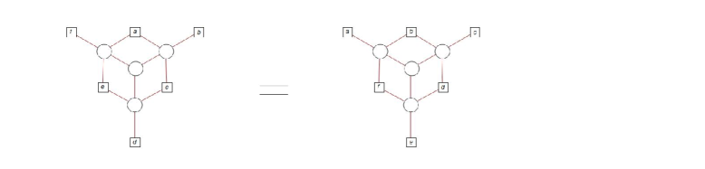
Figure 1. Duality of quiver diagrams.

The ordinary superconformal index of the “theory A” with enhanced symmetry was presented in [17] (see also [28] for the $N_{f}=4$ case and [25, 26] for the similar theory with the broken gauge group). The duality between theories A and B leads to the equality of corresponding superconformal indices expressed by the following $q$-hypergeometric identity [27] (after denoting $x^{2}=q$)

$$\sum_{m\in\mathbb{Z}}\int_{\mathbb{T}}\;q^{-|m|}\;\prod_{j=1}^{6}\frac{(q^{1+\frac{n_{j}}{2}+\frac{|m|}{2}}\frac{1}{a_{j}z},q^{1+\frac{n_{j}}{2}+\frac{|m|}{2}}\frac{z}{a_{j}};q)_{\infty}}{(q^{\frac{n_{j}}{2}+\frac{|m|}{2}}a_{j}z,q^{\frac{n_{j}}{2}+\frac{|m|}{2}}\frac{a_{j}}{z};q)_{\infty}}(1-q^{|m|}z^{2})(1-q^{|m|}z^{-2})\frac{dz}{2\pi iz}$$

$$\qquad\qquad\qquad=\frac{1}{\prod_{j=1}^{6}a_{j}^{n_{j}}}\prod_{1\leq j<k\leq 6}\frac{(q^{1+\frac{n_{j}}{2}+\frac{n_{k}}{2}}a_{j}^{-1}a_{k}^{-1};q)_{\infty}}{(q^{\frac{n_{j}}{2}+\frac{n_{k}}{2}}a_{j}a_{k};q)_{\infty}},$$ (8.14)

with the balancing condition

$$\prod_{j=1}^{6}a_{j}=q,\;\;\text{and}\;\;\sum_{j=1}^{6}n_{j}=0\;.$$ (8.15)

This condition is imposed by the effective superpotential $W=\eta X$ for the theory A, where $X$ is a monopole operator and $\eta$ is the four-dimensional instanton factor, which breaks a part of the symmetry (for details, see [1]). Using the relation [18]

$$\prod_{i=0}^{\infty}\frac{1-q^{i-\frac{1}{2}m+1}z^{-1}}{1-q^{i-\frac{1}{2}m}z}\ =\ (-q^{\frac{1}{2}})^{\frac{1}{2}(m+|m|)}z^{-\frac{1}{2}(m+|m|)}\prod_{i=0}^{\infty}\frac{1-q^{i+\frac{1}{2}|m|+1}z^{-1}}{1-q^{i+\frac{1}{2}|m|}z}$$ (8.16)

one can obtain the $q$-beta sum-integral (2.4) from (8.14).

Similarly, the full symmetry transformation (6.3) is a consequence of a duality of two $3d$ theories with $N_{f}=8$. One can guess that there exist proper analogs of all elliptic hypergeometric integral identities described in [48, 50, 51, 52] for sums of $q$-hypergeometric integrals associated with $3d$ dualities. Actually, the latter dualities are easily found using the reduction of $4d$ superconformal indices to $3d$ partition functions [21] which naturally leads to conjectural equalities of corresponding $3d$ superconformal indices.

By breaking the flavor symmetry to $SU(2)\times SU(2)\times SU(2)$ in (8.14) we obtain the star-triangle relation (7.20). Then the expression (7.19) corresponds to the generalized superconformal index of a $3d$ ${\mathcal{N}}=2$ theory with the gauge group $G=SU(2)$ and the flavor group $F=SU(2)\times SU(2)\times SU(2)\times SU(2)$. In this picture, the SOS-type YBE (7.15) is nothing else than the equality of superconformal indices of two dual $3d$ ${\mathcal{N}}=2$ supersymmetric quiver gauge theories presented in Fig. 1, where the boxes correspond to $SU(2)$ flavor subgroups and the circles represent $SU(2)$ gauge subgroups.

We note that relation (4.5) describes the chiral symmetry breaking similarly to the $3d$ partition function case [54]. Indeed, it assumes the following sum-integral evaluation

$$\sum_{m\in\mathbb{Z}}\int[d_{m}z]\;\Gamma_{q}(t^{-1}x^{\pm 1},\pm n;z,m)\Gamma_{q}(ty^{\pm 1},\pm j;z,m)$$

$$\qquad=\frac{\delta(\phi_{y}+\phi_{x})\delta_{n+j,0}+\delta(\phi_{y}-\phi_{x})\delta_{n-j,0}}{q^{-j}(1-q^{j}y^{2})(1-q^{j}y^{-2})(1-t^{2})(1-t^{-2})},$$ (8.17)

where $y=e^{2\pi i\phi_{y}}$ and $x=e^{2\pi i\phi_{x}}$ and $\delta(\phi)$ is the periodic Dirac delta function with period 1, $\delta(\phi+1)=\delta(\phi)$. On the left-hand side of equality (8.17) we have the $3d$ superconformal index of a theory with $SU(2)$ gauge group and $N_{f}=4$ chiral fields with the naive flavor group $SU(2)\times SU(2)$. However, as follows from the the right-hand side expression, the true flavor group is $(SU(2)\times SU(2))_{diag}$ and the superconformal index has, actually, a non-zero support only on the corresponding subset of fugacities. This is precisely the manifestation of chiral symmetry breaking in confining theories similar to the $3d$ partition functions case [54]. A more detailed and rigorous consideration of this relation between indices and spontaneous breaking of global symmetries is needed, in particular, for the case when one has originally the full naive $SU(4)$ flavor group which is broken to $SP(4)$ group.

Acknowledgements. The authors are indebted to H. Rosengren for helpful discussions. This work is supported by the Heisenberg-Landau program and the Russian foundation for basic research (grant no. 14-01-00474). The research of IG is supported in part by the SFB 647 “Raum-Zeit-Materie. Analytische und Geometrische Strukturen”, the Research Training Group GK 1504 “Mass, Spectrum, Symmetry” and the International Max Planck Research School for Geometric Analysis, Gravitation and String Theory. After completion of this work we have known that the functional form of the star-triangle relation of Sect. 5 was considered in [34] and a relation of $3d$ superconformal indices to integrable lattice systems was discussed in [58].

References

• [1] O.ย Aharony, S.ย S.ย Razamat, N.ย Seiberg and B.ย Willett, 3d dualities from 4d dualities, JHEP 1307, 149 (2013) [arXiv:1305.3924 [hep-th]].
• [2] G. E. Andrews, R. Askey, and R. Roy, Special Functions, Encyclopedia of Math. Appl. 71, Cambridge Univ. Press, Cambridge, 1999.
• [3] R.ย J.ย Baxter, Exactly Solved Models in Statistical Mechanics, Academic Press, London, 1982.
• [4] R.ย J.ย Baxter, Free-fermion, checkerboard and $Z$-invariant lattice models in statistical mechanics, Proc. R. Soc. Lond. A 404 (1986), 1โ€“33.
• [5] R.ย J.ย Baxter, Star-triangle and star-star relations in statistical mechanics, J. Mod. Phys. B 11 (1997), 27โ€“37.
• [6] R.ย J.ย Baxter, The inversion relation method for some two-dimensional exactly solved models in lattice statistics, J. Stat. Phys. 28 (1982), 1โ€“41.
• [7] V.ย V.ย Bazhanov, V.ย V.ย Mangazeev and S.ย M.ย Sergeev, Faddeev-Volkov solution of the Yang-Baxter equation and discrete conformal symmetry, Nucl. Phys. B 784 (2007), 234โ€“258; hep-th/0703041.
• [8] V. V. Bazhanov and S. M. Sergeev, A master solution of the quantum Yang-Baxter equation and classical discrete integrable equations, ATMP 16 (2012), 65โ€“95.
• [9] S. Benvenuti, B. Feng, A. Hanany, and Y.-H. He, Counting BPS Operators in Gauge Theories: Quivers, Syzygies and Plethystics, JHEP 0711 (2007) 050, arXiv:hep-th/0608050 [hep-th].
• [10] J. Bhattacharya and S. Minwalla, Superconformal Indices for $N=6$ Chern Simons Theories, JHEP 0901 (2009) 014, arXiv:0806.3251 [hep-th].
• [11] D. Chicherin, S.E. Derkachov, V.P. Spiridonov, New elliptic solutions of the Yang-Baxter equation, arXiv:1412.3383 [math-ph].
• [12] E. Date, M. Jimbo, A. Kuniba, T. Miwa and M. Okado, Exactly solvable SOS models: local height probabilities and theta function identities, Nucl. Phys B 290 (1987), 231โ€“273.
• [13] E. Date, M. Jimbo, A. Kuniba, T. Miwa and M. Okado, Exactly solvable SOS models II: Proof of the star-triangle relation and combinatorial identities, in Conformal field theory and lattice models, M. Jimbo, T. Miwa and A. Tsuchiya, eds., Advanced Studies in Pure Math. 16 (1988), 17 122.
• [14] S. E. Derkachov, Factorization of the $R$-matrix. I. Zap. Nauchn. Sem. POMI 335 (2006), 134โ€“163 (J. Math. Sciences 143 (1) (2007), 2773-2790), math-qa/0503396.
• [15] S. E. Derkachov and A. N. Manashov, General solution of the Yang-Baxter equation with the symmetry group $\mathrm{SL}(n,\mathbb{C})$, Algebra i Analiz 21 (4) (2009), 1โ€“94 (St. Petersburg Math. J. 21 (2010), 513โ€“577).
• [16] S. E. Derkachov and V. P. Spiridonov, Yang-Baxter equation, parameter permutations, and the elliptic beta integral, Uspekhi Mat. Nauk 68 (6) (2013), 59โ€“106 (Russian Math. Surveys 68 (6) (2013), 1027โ€“1072); arXiv:1205.3520 [math-ph].
• [17] T. Dimofte and D. Gaiotto, An $E_{7}$ Surprise, JHEP 1210 (2012), 129, arXiv:1209.1404 [hep-th].
• [18] T. Dimofte, D. Gaiotto, and S. Gukov, 3-Manifolds and 3d Indices, Adv. Theor. Math. Phys. 17 (2013) 975-1076, arXiv:1112.5179 [hep-th].
• [19] F. Dolan, On Superconformal Characters and Partition Functions in Three Dimensions, J. Math. Phys. 51 (2010), 022301, arXiv:0811.2740 [hep-th].
• [20] F.ย A.ย Dolan and H.ย Osborn, Applications of the Superconformal Index for Protected Operators and $q$-Hypergeometric Identities to $\mathcal{N}=1$ Dual Theories, Nucl. Phys. B 818 (2009), 137โ€“178.
• [21] F.ย A.ย H.ย Dolan, V.ย P.ย Spiridonov, and G.ย S.ย Vartanov, From $4d$ superconformal indices to $3d$ partition functions, Phys. Lett. B 704 (2011), 234โ€“241.
• [22] N. Drukker, T. Okuda, and F. Passerini, Exact results for vortex loop operators in $3d$ supersymmetric theories, JHEP 1407 (2014) 137, arXiv:1211.3409 [hep-th].
• [23] L. D. Faddeev, How algebraic Bethe ansatz works for integrable model, Quantum Symmetries, Proc. Les-Houches summer school, LXIV, North-Holland, 1998, 149โ€“211.
• [24] B. Feng, A. Hanany, and Y.-H. He, Counting gauge invariants: The Plethystic program, JHEP 0703 (2007) 090, arXiv:hep-th/0701063 [hep-th].
• [25] I.ย Gahramanov and H.ย Rosengren, A new pentagon identity for the tetrahedron index, JHEP 1311, 128 (2013) arXiv:1309.2195 [hep-th].
• [26] I.ย Gahramanov and H.ย Rosengren, Integral pentagon relations for 3d superconformal indices, arXiv:1412.2926 [hep-th].
• [27] I.ย Gahramanov H.ย Rosengren, Basic hypergeometry of SUSY dualities, in preparation.
• [28] I. Gahramanov and G. Vartanov, Extended global symmetries for $4D$ $N=1$ SQCD theories, J. Phys. A: Math. Theor. 46 (2013), 285403, arXiv:1303.1443 [hep-th].
• [29] N.ย Hama, K.ย Hosomichi, and S.ย Lee, SUSY gauge theories on squashed three-spheres, JHEP 1105 (2011), 014.
• [30] Y. Imamura and S. Yokoyama, Index for three dimensional superconformal field theories with general R-charge assignments, JHEP 1104 (2011) 007, arXiv:1101.0557 [hep-th].
• [31] M. Jimbo (ed), Yang-Baxter equation in integrable systems, Adv. Ser. Math. Phys., 10, World Scientific (Singapore), 1990.
• [32] A. Kapustin and B. Willett, Generalized Superconformal Index for Three Dimensional Field Theories, arXiv:1106.2484 [hep-th].
• [33] A. P. Kels, A new solution of the star-triangle relation, J. Phys. A: Math. Theor. 47 (2014), 055203.
• [34] A.ย P.ย Kels, New solutions of the star-triangle relation with discrete and continuous spin variables, arXiv:1504.07074 [math-ph].
• [35] S. Kim, The complete superconformal index for N=6 Chern-Simons theory, Nucl. Phys. B 821 (2009) 241-284, arXiv:0903.4172 [hep-th].
• [36] J. Kinney, J. M. Maldacena, S. Minwalla and S. Raju, An index for 4 dimensional super conformal theories, Commun. Math. Phys. 275 (2007), 209โ€“254.
• [37] C. Krattenthaler, V.P. Spiridonov, and G.S. Vartanov, Superconformal indices of three-dimensional theories related by mirror symmetry, JHEP 1106 (2011) 008, arXiv:1103.4075 [hep-th].
• [38] V. Pestun, Localization of gauge theory on a four-sphere and supersymmetric Wilson loops, Commun. Math. Phys. 313 (2012) 71-129, arXiv:0712.2824 [hep-th].
• [39] L. Rastelli and S. S. Razamat, The superconformal index of theories of class $\mathcal{S}$, arXiv:1412.7131.
• [40] C. Rรถmelsberger, Counting chiral primaries in ${\mathcal{N}}=1$, $d=4$ superconformal field theories, Nucl. Phys. B 747 (2006), 329โ€“353.
• [41] C. Rรถmelsberger, Calculating the superconformal index and Seiberg duality, arXiv:0707.3702 [hep-th].
• [42] H.ย Rosengren, Askey-Wilson polynomials and the tetrahedron index, talk at Conference for Dick Askeyโ€™s 80th Birthday, 6โ€“7 December, 2013, Madison, Wisconsin, USA; http://www.math.umn.edu/$\sim$stant001/ASKEYABS/Hjalmar$\_$Rosengren.pdf
• [43] N.ย Seiberg, Exact Results On The Space Of Vacua Of Four-Dimensional Susy Gauge Theories, Phys. Rev. D 49 (1994), 6857โ€“6863.
• [44] N. Seiberg, Electricโ€“magnetic duality in supersymmetric non-Abelian gauge theories, Nucl. Phys. B 435 (1995), 129โ€“146.
• [45] V. P. Spiridonov, On the elliptic beta function, Uspekhi Mat. Nauk 56 (1) (2001), 181โ€“182 (Russian Math. Surveys 56 (1) (2001), 185โ€“186).
• [46] V. P. Spiridonov, Theta hypergeometric integrals, Algebra i Analiz 15 (6) (2003), 161โ€“215 (St. Petersburg Math. J. 15 (6) (2004), 929โ€“967).
• [47] V. P. Spiridonov, A Bailey tree for integrals, Teor. Mat. Fiz. 139 (2004), 104โ€“111 (Theor. Math. Phys. 139 (2004), 536โ€“541); math.CA/0312502.
• [48] V. P. Spiridonov, Elliptic hypergeometric functions, Habilitation thesis, Laboratory of Theoretical Physics, JINR, September 2004; Essays on the theory of elliptic hypergeometric functions, Uspekhi Mat. Nauk 63 (3) (2008), 3โ€“72 (Russian Math. Surveys 63 (3) (2008), 405โ€“472).
• [49] V. P. Spiridonov, Elliptic beta integrals and solvable models of statistical mechanics, Contemp. Math. 563 (2012), 181โ€“211; arXiv:1011.3798 [hep-th].
• [50] V. P. Spiridonov and G. S. Vartanov, Superconformal indices for ${\mathcal{N}}=1$ theories with multiple duals, Nucl. Phys. B 824 (2010), 192โ€“216.
• [51] V. P. Spiridonov and G. S. Vartanov, Elliptic hypergeometry of supersymmetric dualities, Commun. Math. Phys. 304 (2011), 797โ€“874
• [52] V. P. Spiridonov and G. S. Vartanov, Elliptic hypergeometry of supersymmetric dualities II. Orthogonal groups, knots, and vortices, Commun. Math. Phys. 325 (2014), 421โ€“486.
• [53] V.ย P.ย Spiridonov and G.ย S.ย Vartanov, Elliptic hypergeometric integrals and โ€™t Hooft anomaly matching conditions, JHEP 06 (2012), 016.
• [54] V.ย P.ย Spiridonov and G.ย S.ย Vartanov, Vanishing superconformal indices and the chiral symmetry breaking, J. High Energy Phys. 06 (2014), 062; arXiv:1402.2312 [hep-th].
• [55] L.โ€‰A.ย Takhtadzhan, L.โ€‰D.ย Faddeev, The quantum method of inverse problem and the Heisenberg XYZ model, Uspekhi Mat. Nauk 34 (5) (1979), 13โ€“63 (Russian Math. Surveys 34 (5) (1979), 11โ€“68).
• [56] J. Teschner and G. Vartanov, $6j$ symbols for the modular double, quantum hyperbolic geometry, and supersymmetric gauge theories, Lett. Math. Phys. 104 (2014) 527-551, arXiv:1202.4698 [hep-th].
• [57] A. Yu. Volkov and L. D. Faddeev, Yang-Baxterization of the quantum dilogarithm, Zapiski Nauch. Sem. POMI 224 (1995), 146โ€“154 (J. Math. Sciences 88 (2) (1998), 202โ€“207).
• [58] J. Yagi, Quiver gauge theories and integrable lattice models, arXiv:1504.04055 [hep-th].