Hamiltonian tomography for quantum many-body systems with arbitrary couplings

Abstract

Characterization of qubit couplings in many-body quantum systems is essential for benchmarking quantum computation and simulation. We propose a tomographic measurement scheme to determine all the coupling terms in a general many-body Hamiltonian with arbitrary long-range interactions, provided the energy density of the Hamiltonian remains finite. Different from quantum process tomography, our scheme is fully scalable with the number of qubits as the required rounds of measurements increase only linearly with the number of coupling terms in the Hamiltonian. The scheme makes use of synchronized dynamical decoupling pulses to simplify the many-body dynamics so that the unknown parameters in the Hamiltonian can be retrieved one by one. We simulate the performance of the scheme under the influence of various pulse errors and show that it is robust to typical noise and experimental imperfections.

Introduction.—Physicists have been striving to understand and harness the power of quantumness since the establishment of the quantum theory. With the flourishing of quantum information science in recent decades Nielsen and Chuang (2010); Ladd et al. (2010), numerous breakthroughs—both in theory and in experiment—helped to frame a clearer goal: it is the entanglement and the exponentially growing Hilbert space that distinguishes quantum many-body systems from classical systems Feynman (1982); Horodecki et al. (2009); Cirac and Zoller (2012). To fully leverage the quantum supremacy, a vital step is to verify and benchmark the quantum device. The standard techniques of quantum state and process tomography Vogel and Risken (1989); Smithey et al. (1993); Chuang and Nielsen (1997); James et al. (2001); Haffner et al. (2005); Lvovsky and Raymer (2009), however, are plagued by the same exponential growth of dimensions Paris and Rehacek (eds). A related problem is to directly identify Hamiltonians, the generators of quantum dynamics. They can often be specified by fewer number of parameters that scales polynomially with the system size.

Hamiltonian tomography for generic many-body systems is nevertheless a daunting task. The way to extract information of unknown parameters in a Hamiltonian is by measuring certain features of its generated dynamics. To make this possible, one has to solve the dynamics generated by the Hamiltonian to make a definite connection between its dynamical features and the Hamiltonian parameters. However, for general many-body Hamiltonians, their dynamics are extremely complicated and intractable by numerical simulation as the simulation time increases exponentially with the size of the system. Progress in this direction has mostly be on small systems Schirmer et al. (2004); Cole et al. (2005, 2006); Devitt et al. (2006); Senko et al. (2014) or special many-body systems which are either exactly solvable due to many conserved operators, of limited Hilbert space dimensions amenable to numerical simulation, or short-range interacting systems Burgarth and Maruyama (2009); Burgarth et al. (2009, 2011); Di Franco et al. (2009); Zhang and Sarovar (2014); da Silva et al. (2011); Wiebe et al. (2014).

In this paper, we propose a scheme to achieve Hamiltonian tomography for general many-body Hamiltonians with arbitrary long-range couplings between the qubits. The key idea is to simplify the dynamics generated by a general many-body Hamiltonian through application of a sequence of dynamical decoupling pulses on individual qubits. Dynamical decoupling (DD) is a powerful technique that uses periodic fast pulses to suppress noise and average out unwanted couplings between the system and the environment Gullion et al. (1990); Viola and Lloyd (1998); Viola et al. (1999); Duan and Guo (1999); Zanardi (1999); Khodjasteh and Lidar (2005, 2007); Uhrig (2007); Yang et al. (2011); Souza et al. (2011, 2012); Álvarez et al. (2010); Morton et al. (2006); Biercuk et al. (2009); Du et al. (2009); West et al. (2010). We apply a sequence of synchronized DD pulses on a pair of qubits, which forms a small target system that has coupling with the rest of the qubits in the many-body Hamiltonian, the effective environment. The DD pulses keep the desired couplings within this target system intact while average out its couplings with all the environment qubits. The dynamics under the DD pulses become exactly solvable, from which we can perform a tomographic measurement to determine the coupling parameters within this small target system Schirmer et al. (2004); Cole et al. (2005, 2006); Devitt et al. (2006). We then scan the DD pulses to different pairs of qubits to measure all the other coupling terms in the Hamiltonian. We assume the ability to address individual qubits, which is realistic for many experimental platforms, such as trapped ions Schmidt-Kaler et al. (2003); Johanning et al. (2009); Crain et al. (2014), cold atoms Sherson et al. (2010); Bakr et al. (2010); Weitenberg et al. (2011), and solid-state qubit systems Devoret and Schoelkopf (2013); Barends et al. (2014, 2015); Salathé et al. (2015). Several features make the scheme amenable to experimental implementation. First of all, applying the DD pulse sequence is a standard procedure in many experiments. Post-processing of data is straightforward as it only requires one or two parameter curve fitting. In addition, we demonstrate with explicit numerical simulation that the scheme is robust to various sources of errors in practical implementation, such as the remnant DD coupling error, measurement uncertainties, and different types of pulse errors.

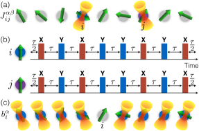
Figure 1: (color online). Schematics for the tomography procedure. (a) To map out the coupling coefficients $J_{ij}^{\alpha\beta}$, a synchronized DD sequence is applied to spins $i$ and $j$. Both spins will be decoupled from the rest of the system. (b) The $XY$-$8$ DD sequence on spins $i$ and $j$ to probe the parameters of the Hamiltonian in Eq. (3). The initial state is for instance prepared to the $|00\rangle$ state for the two spins. (c) To retrieve information about the local fields $b_{i}^{\alpha}$, $XY$-$8$ pulse sequences are applied to the environment spins to decouple spin $i$ from the rest.

Scheme for Hamiltonian tomography.—The system we have in mind is the most general Hamiltonian with two-body qubit interactions

$$H=\sum_{\alpha,\beta,m<n}J_{mn}^{\alpha\beta}\sigma_{m}^{\alpha}\sigma_{n}^{\beta}+\sum_{m,\alpha}b_{m}^{\alpha}\sigma_{m}^{\alpha},$$ (1)

where $J_{mn}^{\alpha\beta}$ characterizes the coupling strength between spins $m$ and $n$ for the $\alpha,\beta$ components, and $b_{m}^{\alpha}$ represents the local field on spin $m$; $\sigma^{\alpha}\left(\sigma^{\beta}\right)$ are the Pauli matrices along the $\alpha$ $(\beta)$ direction with $\alpha,\beta\in(x,y,z)$. To adopt consistent notations throughout the text, we use $m,n$ to denote a general spin label and $i,j$ to refer to the specific target spins that we are probing with the DD pulses, calling the rest of the spins as environment spins. The terms spin and qubit are used interchangeably. Let the energy unit of the Hamiltonian be $J$, chosen to be the largest magnitude of all coefficients, so $J_{mn}^{\alpha\beta}/J$ and $b_{m}^{\alpha}/J$ are bounded between $-1$ and $1$. In order to map out the coupling coefficient $J_{ij}^{\alpha\beta}$ for the target spins, we propose to decouple these two spins from the environment spins by a synchronized DD pulse sequence. A synchronized $XY$-$4$ sequence applied to both spins will average out their interactions with other spins while preserving the two-spin coherence (see Fig. 1(a-b) for the schematic and the pulse sequence). Basically, only those interactions that commute with the DD sequence will survive. More rigorously, the evolution operator in one period is

$$U_{1} =U_{0}^{1/2}\sigma_{i}^{x}\sigma_{j}^{x}U_{0}\sigma_{i}^{y}\sigma_{j}^{y}U_{0}\sigma_{i}^{x}\sigma_{j}^{x}U_{0}\sigma_{i}^{y}\sigma_{j}^{y}U_{0}^{1/2}$$

$$=e^{-i4\tau(J_{ij}^{xx}\sigma_{i}^{x}\sigma_{j}^{x}+J_{ij}^{yy}\sigma_{i}^{y}\sigma_{j}^{y}+J_{ij}^{zz}\sigma_{i}^{z}\sigma_{j}^{z}+B)+O(J^{2}\tau^{2})},$$ (2)

where $U_{0}=e^{-iH\tau}$, $\tau$ is the time interval between two consecutive pulses, and $B$, the bath, includes all terms of the Hamiltonian that only acts on environment spins. See Supplemental Material for the detailed derivation Ham . To bound the error term to $O(J^{2}\tau^{2})$, we assume $\sum_{n}J_{in}^{\alpha\beta}=O(J)$, i.e., the interaction strength decays rapidly with spin separation distance so that the energy density of the Hamiltonian is bounded by a constant. This condition is satisfied for any finite systems as in the experiment with arbitrary interactions. In the thermodynamic limit, it is also a reasonable assumption for any physical systems whose energy is extensive. It may also be related to the generalized Lieb-Robinson bound for systems with long-range interactions Hastings and Koma (2006); Nachtergaele and Sims (2006); Gong et al. (2014); Foss-Feig et al. (2015). The $XY$-$8$ pulse sequence, which is the concatenation of $XY$-$4$ sequence with its time-reversal, eliminates the error term to the third order $O(J^{3}\tau^{3})$. Fig. 1(b) shows the $XY$-$8$ DD pulse sequence. Hence, in the Hilbert subspace of the target spins, the effective Hamiltonian is

$$H_{2\text{-spin}}=c_{1}\sigma_{i}^{x}\sigma_{j}^{x}+c_{2}\sigma_{i}^{y}\sigma_{j}^{y}+c_{3}\sigma_{i}^{z}\sigma_{j}^{z},$$ (3)

where we use $c_{1}\equiv J_{ij}^{xx},c_{2}\equiv J_{ij}^{yy},c_{3}\equiv J_{ij}^{zz}$ to simplify the notation. The effective two-spin unitary evolution after $N_{c}$ cycles of $XY$-$8$ sequence is

$$U_{2\text{-spin}}=$$

$$\!\!\left(\begin{array}[]{cccc}\!\tfrac{\cos\left((c_{1}-c_{2})T\right)}{e^{ic_{3}T}}&\!0&\!0&\!\tfrac{\sin\left((c_{1}-c_{2})T\right)}{ie^{ic_{3}T}}\\ \!0&\!\tfrac{\cos\left((c_{1}+c_{2})T\right)}{e^{-ic_{3}T}}&\!\tfrac{\sin\left((c_{1}+c_{2})T\right)}{ie^{-ic_{3}T}}&\!0\vspace{0.1cm}\\ \!0&\!\tfrac{\sin\left((c_{1}+c_{2})T\right)}{ie^{-ic_{3}T}}&\!\tfrac{\cos\left((c_{1}+c_{2})T\right)}{e^{-ic_{3}T}}&\!0\\ \!\tfrac{\sin\left((c_{1}-c_{2})T\right)}{ie^{ic_{3}T}}&\!0&\!0&\!\tfrac{\cos\left((c_{1}-c_{2})T\right)}{e^{ic_{3}T}}\end{array}\!\right),$$

where $T=8N_{c}\tau$ is the total time. From the above expression, one may notice that the Hamiltonian parameters can be retrieved by preparing a particular initial state and measuring its time-evolved output probability in a given basis. In particular, we have

$$P_{|+\text{I}\rangle\rightarrow|00\rangle} =\left|\langle 00|U_{2\text{-spin}}|\!+\!\text{I}\rangle\right|^{2}=\tfrac{1}{4}\left[1+\sin(2(c_{1}-c_{2})T)\right]$$

$$P_{|+\text{I}\rangle\rightarrow|10\rangle} =\left|\langle 10|U_{2\text{-spin}}|\!+\!\text{I}\rangle\right|^{2}=\tfrac{1}{4}\left[1+\sin(2(c_{1}+c_{2})T)\right]$$

$$P_{|0\text{I}\rangle\rightarrow|++\rangle} =\left|\langle+\!+\!|U_{2\text{-spin}}|0\text{I}\rangle\right|^{2}\!=\!\tfrac{1}{4}\left[1+\sin(2(c_{2}-c_{3})T)\right]$$

where $|+\rangle=\frac{1}{\sqrt{2}}(|0\rangle+|1\rangle)$ and $|\text{I}\rangle=\frac{1}{\sqrt{2}}(|0\rangle+i|1\rangle)$ are the rotated basis. The coupling strengths $c_{1},c_{2}$ and $c_{3}$ can be extracted from the oscillation frequencies of these three sets of measurements at various time points. These particular sets are not the only suite to extract those parameters. They are chosen for the convenience in fitting and in state preparation. Only product states of the two target spins, disentangled from the rest, are required. We also remark that the error incurred is $O(N_{c}J^{3}\tau^{3})$, so one needs $J\tau\ll 1$ for a robust decoupling scheme. In a similar fashion, one can retrieve all other coupling coefficients. Let us denote the synchronized $XY$-$8$ DD pulse sequence as $X_{i}X_{j}$-$Y_{i}Y_{j}$-$8$ to show explicitly the particular pulses on specific spins. Replacing the sequence with $X_{i}Y_{j}$-$Y_{i}Z_{j}$-8 ($Y_{i}X_{j}$-$Z_{i}Y_{j}$-8) pulses, we will be able to extract the coefficients $J_{ij}^{xy},J_{ij}^{yz}$ and $J_{ij}^{zx}$ ($J_{ij}^{yx},J_{ij}^{xz}$ and $J_{ij}^{zy}$), respectively.

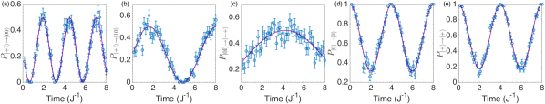
Figure 2: (color online). Numerical simulation and curving fitting results. (a)-(c) are used to retrieve $J_{79}^{xx}$, $J_{79}^{yy}$ and $J_{79}^{zz}$ between spins 7 and 9. (d) and (e) are used to extract $b_{6}^{x}$, $b_{6}^{y}$ and $b_{6}^{z}$ for spin 6. Each measurement data $p_{m}$ are drawn from the binomial distribution with the true probability $p$ as the mean and $p(1-p)/N_{m}$ as the variance. The measurement uncertainty of each point is thus $\sqrt{p_{m}(1-p_{m})/N_{m}}$. The blue solid lines are the best-fit lines with the simulated experimental data $p_{m}$, and red dashed lines are the theoretical ones generated by the true Hamiltonian parameters. Pulse errors are not included in these plots, so any discrepancies stem from the remnant DD coupling error and measurement uncertainties. Other parameters used are $N=12$, $\tau J=0.01$, $N_{m}=100$, $N_{t}=50$.

By scanning the DD pulses to different target pairs, the above procedure recovers all the coupling coefficients $J_{mn}^{\alpha\beta}$. The retrieval of local field coefficients follows a similar approach. We now need to decouple the particular spin $i$ from the rest without contaminating its own spin term $b_{i}^{\alpha}\sigma_{i}^{\alpha}$. Shining a $XY$-$8$ DD sequence on spin $i$ removes all information about $b_{i}^{\alpha}$ too. Instead, one could address all the environment spins with $XY$-$8$ pulses, and decouple them from spin $i$ (alternative schemes are discussed in the Supplemental Material Ham ). This scheme will be very robust to pulse errors, since no laser pulses are directly applied to the target spin [Fig. 1(c)]. The effective single-spin Hamiltonian is thus $H_{1\text{-spin}}=b_{i}^{x}\sigma_{i}^{x}+b_{i}^{y}\sigma_{i}^{y}+b_{i}^{z}\sigma_{i}^{z}$ with a unitary evolution $U_{1\text{-spin}}=e^{-iH_{1\text{-spin}}T}$ executing a spin rotation on the Bloch sphere. Again, by preparing a particular state and measuring its time evolution, we get $P_{|0\rangle\rightarrow|0\rangle}=1+\left[\left(b_{i}^{z}/b\right)^{2}-1\right]\sin^{2}(bT)$ and $P_{|+\rangle\rightarrow|+\rangle}=1+\left[\left(b_{i}^{x}/b\right)^{2}-1\right]\sin^{2}(bT)$, where $b=\sqrt{(b_{i}^{x})^{2}+(b_{i}^{y})^{2}+(b_{i}^{z})^{2}}$ is the magnitude of the Bloch vector. These two sets of measurements will determine $b_{i}^{x},b_{i}^{y}$ and $b_{i}^{z}$ up to a sign. The correct signs from the remaining discrete set can be picked out by measuring $P_{|+\rangle\rightarrow|0\rangle}$ and $P_{|\text{I}\rangle\rightarrow|0\rangle}$ at a single time point Ham .

The complete scheme applies to any generic Hamiltonian with interacting qubits. In the most general case, one needs to determine $9N(N-1)/2+3N$ coefficients. However, in many physical systems, the particular form of the interaction is known and/or the interaction often decays fast enough that one can significantly reduce the number of measurements required. In particular, if $J_{mn}^{\alpha\beta}$ can be truncated at some spin separation distance in the case of short-range interactions, the number of measurements will be linear with the system size $N$. In the following, we numerically simulate the experimental procedure for the most general Hamiltonian, taking into account various sources of errors, including the remnant DD coupling error, measurement uncertainties, and different forms of pulse errors.

Numerical simulation.—We consider the general Hamiltonian given in Eq. (1) with coefficients $J_{ij}^{\alpha\beta}/J$ and $b_{i}^{\alpha}/J$ randomly drawn from $-1$ to $1$. In our finite-system simulation, we ignore the decay of $J_{ij}^{\alpha\beta}$ with distance, so the system may include unphysically long-range interactions and could simulate Hamiltonians in any dimensions. To retrieve $J_{ij}^{\alpha\alpha}$, for example, we start with a product state of all spins, and perform time evolution using the entire Hamiltonian from Eq. (1), interspersed with the $XY$-$8$ DD pulses on target spins $i$ and $j$. We would like to emphasize that specific state initialization for the environment spins is not required as long as they are disentangled from the target pair of qubits at the beginning. After $N_{c}$ cycles of the DD sequence, the environment spins are traced out and measurements are made on spins $i$ and $j$. In the simulation, we do not assume the pure unitary evolution $U_{2\text{-spin}}$ as the remnant coupling to the environment spins may entangle the two spins with the rest. However, any undesired couplings are suppressed to the order of $O(J^{3}\tau^{3})$ and we do observe that the two-spin density matrix remains mostly pure ($\sim 99.9\%$) for our chosen parameters.

As the tomography procedure involves measuring the output probability of a certain state, each time point will be measured $N_{m}$ times, which gives an estimate of the probability $p_{m}$ in this state. The measurement uncertainty (standard deviation) will be $\sqrt{p_{m}(1-p_{m})/N_{m}}$ following the binomial distribution. As discussed above, to map out $c_{1},c_{2}$ and $c_{3}$, one needs to measure $P_{|+\text{I}\rangle\rightarrow|00\rangle},P_{|+\text{I}\rangle\rightarrow|10\rangle}$ and $P_{|0\text{I}\rangle\rightarrow|++\rangle}$ for the target spins at various time points and extract the corresponding oscillation frequencies. Suppose $N_{t}$ different time points are measured for each set. The oscillation frequencies can be found either by Fourier transform or by curve fitting. In general, if data show numerous oscillation periods, Fourier transform will be more robust and reliable Cole et al. (2005, 2006); Devitt et al. (2006). In our case, however, the long time observations will be undermined by the remnant coupling to the environment spins and possible pulse error accumulation. Simple curving fitting with fewer oscillation periods, therefore, appears to be a better solution. In Fig. 2(a-c), we fit the data with the method of least squares with $\tau J=0.01,N_{m}=100,N_{t}=50$ for spins $i=7$ and $j=9$ in a $N=12$ spin system. The blue solid lines are the best-fit lines, and the red dashed lines are the theoretical lines using the true coupling coefficients. The longest time period requires $800$ pulses, which is well within the current experimental technology without significant pulse error accumulation. Table 1 compares the true values and the estimated ones of $J_{79}^{\alpha\alpha}$. Uncertainties in the estimation stem from the curve fitting due to measurement uncertainties. Corresponding results for $b_{6}^{\alpha}$ of spin $6$ are shown in Fig. 2(d-e) and Table 1. All estimated parameters are accurate within a few percent.

To simulate real experiments, one also needs to include possible pulse errors. One possible source of errors is the finite duration of each control pulse, which limits the minimum cycle time. This is typically not the dominant source of errors and can often be well-controlled Khodjasteh and Lidar (2007); Viola and Knill (2003); Souza et al. (2012); Hodgson et al. (2010); Uhrig and Pasini (2010). In most experiments, the major cause of errors is the deviation between the control pulses and the ideal $X$ or $Y$ pulses. These can either arise from the amplitude error where the rotation angle differs from the ideal $\pi$-pulse or the rotation error where the rotation axis deviates from the $x$ or $y$ axis. In typical experiments, individual pulse errors may be controlled within a percent level. In our simulation, we consider three different forms of pulse errors: Systematic Amplitude pulse Error (SAE), Random Amplitude pulse Error (RAE) and Random Rotation axis Error (RRE). See the caption of Table 1 for the specific forms of the errors. Moderate systematic errors can be self-compensated by the $XY$-$8$ DD sequence. Numerically, we found that $5\%$ of SAE has negligible effect on the parameter estimation. In addition, we also simulated the cases where each pulse experiences a $1\%$ RAE or RRE. Results are summarized in Table 1. The average deviation from the true parameters are within $5\%$. Here, we would like to point out a few features of our scheme that make it inherently robust to errors. First of all, the estimation of the coupling strength $J_{mn}^{\alpha\beta}$ only entails frequency estimation, which could endure large deviations of a few measurement points. In addition, the single-parameter curve fitting scheme not only makes the estimation robust but is also more convenient for experiment. Moreover, the retrieval of local fields $b_{m}^{\alpha}$ is remarkably tolerant to pulse errors. Since no pulse is directly applied to the target spin, any pulse errors on the environment spins will only be propagated via the remnant DD coupling error, which is suppressed to the order of $O(J^{3}\tau^{3})$. We have numerically tested that a $10\%$ pulse error of any kind would have negligible effects on the estimation of $b_{m}^{\alpha}$. Alternative schemes to extract the local fields are detailed and discussed in the Supplemental Material Ham . They are less tolerant to pulse errors, but may be easier to implement in some experimental setups.

Discussion and outlook.—We have thus numerically demonstrated that the proposed scheme is robust to various sources of errors present in real experiments. The measurement uncertainties can be lowered by increasing $N_{m}$ and the pulse errors can be reduced by limiting the maximum number of pulses needed. The optimal strategy involves a delicate balance between experimental sophistication and error control. For example, by fixing $\tau J$ and the total number of measurements for each set, $N_{m}\times N_{t}$, one could devise an optimal estimation procedure. In addition, it is also possible to eliminate the remnant DD coupling error to a higher order with more elaborate pulse sequences such as the concatenated DD sequence Khodjasteh and Lidar (2005, 2007) and reduce pulse errors by designing composite pulses or self-correcting sequences Souza et al. (2011, 2012); Levitt (1986); Ryan et al. (2010). The scheme can also be extended straightforwardly to qudit systems of higher spins or to bosonic or fermionic systems.

In conclusion, we have proposed a general scheme to achieve full Hamiltonian tomography for generic interacting qubit systems with arbitrary long-range couplings. The required number of measurements scales linearly with the number of terms in the Hamiltonian, and the scheme is robust to typical experimental errors or imperfections.

Table 1: NPE: No Pulse Error; SAE: Systematic Amplitude pulse Error; RAE: Random Amplitude pulse Error; RRE: Random Rotation axis Error; AD: Average Deviation from true values. The last digit in bracket for each number quantifies the estimation error bar due to measurement uncertainties, which is generated by the bootstrapping method. The percentage values in the brackets denote the amount of errors introduced in each pulse. The errors are in the form of: SAE, $e^{i\frac{\pi}{2}(1+\epsilon)\sigma^{\nu}}$; RAE, $e^{i\frac{\pi}{2}(1+\delta)\sigma^{\nu}}$; RRE, $e^{i\frac{\pi}{2}(\sigma^{\nu}+\alpha\sigma^{x}+\beta\sigma^{y}+\gamma\sigma^{z})}$; where $\epsilon=5\%$, $\delta$ is randomly chosen from $(-1\%,1\%)$, $(\alpha,\beta,\gamma)$ is a vector with a random direction but fixed magnitude at $1\%$, and $\nu=x,y$ for the $X$ and $Y$ pulses respectively.

	True	Estimated Parameters
	–	NPE	SAE(5%)	RAE(1%)	RRE(1%)
$J_{79}^{xx}$	$-0.378$	$-0.369(3)$	$-0.377(3)$	$-0.379(4)$	$-0.412(2)$
$J_{79}^{yy}$	0.863	0.856(3)	0.846(3)	0.867(4)	0.836(2)
$J_{79}^{zz}$	0.679	0.669(5)	0.649(5)	0.718(6)	0.611(4)
$b_{6}^{x}$	0.334	0.32(1)	0.32(1)	0.32(1)	0.32(1)
$b_{6}^{y}$	0.569	0.567(8)	0.567(8)	0.567(8)	0.568(8)
$b_{6}^{z}$	$-0.431$	$-0.441(8)$	$-0.443(8)$	$-0.441(8)$	$-0.441(8)$
AD	–	2%	3%	3%	5%

I Supplemental Material: Hamiltonian tomography for quantum many-body systems with arbitrary couplings

In this Supplemental Material, we provide more details on the dynamical decoupling scheme and error estimation, the retrieval of local field parameters and alternative schemes, and include further results taking into account of pulse errors.

II Dynamical Decoupling

The most general Hamiltonian with two-body qubit interactions can be written as

$$H=\sum_{\alpha,\beta,m<n}J_{mn}^{\alpha\beta}\sigma_{m}^{\alpha}\sigma_{n}^{\beta}+\sum_{m,\alpha}b_{m}^{\alpha}\sigma_{m}^{\alpha}.$$ (4)

The energy unit of the Hamiltonian is taken to be $J$ such that $J_{mn}^{\alpha\beta}/J$ and $b_{m}^{\alpha}/J$ are bounded between $-1$ and $1$. The symmetric $XY$-$4$ dynamical decoupling (DD) sequence on both spins $i$ and $j$ produces

$$U_{1}=U_{0}^{1/2}\left(\sigma_{i}^{x}\sigma_{j}^{x}U_{0}\sigma_{i}^{x}\sigma_{j}^{x}\right)\left(\sigma_{i}^{z}\sigma_{j}^{z}U_{0}\sigma_{i}^{z}\sigma_{j}^{z}\right)\left(\sigma_{i}^{y}\sigma_{j}^{y}U_{0}\sigma_{i}^{y}\sigma_{j}^{y}\right)U_{0}^{1/2},$$ (5)

where $U_{0}=e^{-iH\tau}$ and $\tau$ is the time interval between consecutive pulses. We can decompose $H$ into two parts.

$$H =H_{0}+H_{1},$$ (6)

$$H_{0} =J_{ij}^{xx}\sigma_{i}^{x}\sigma_{j}^{x}+J_{ij}^{yy}\sigma_{i}^{y}\sigma_{j}^{y}+J_{ij}^{zz}\sigma_{i}^{z}\sigma_{j}^{z},$$ (7)

$$H_{1} =J_{ij}^{xy}\sigma_{i}^{x}\sigma_{j}^{y}+J_{ij}^{xz}\sigma_{i}^{x}\sigma_{j}^{z}+J_{ij}^{yx}\sigma_{i}^{y}\sigma_{j}^{x}+J_{ij}^{yz}\sigma_{i}^{y}\sigma_{j}^{z}+J_{ij}^{zx}\sigma_{i}^{z}\sigma_{j}^{x}+J_{ij}^{zy}\sigma_{i}^{z}\sigma_{j}^{y}$$

$$+\sigma_{i}^{x}B_{i}^{x}+\sigma_{i}^{y}B_{i}^{y}+\sigma_{i}^{z}B_{i}^{z}+\sigma_{j}^{x}B_{j}^{x}+\sigma_{j}^{y}B_{j}^{y}+\sigma_{j}^{z}B_{j}^{z}+B,$$ (8)

where $B_{i}^{\alpha}$ includes the local field on the $i$th spin and interacting terms between the $i$th spin and all other spins other than the $j$th spin, i.e., $B_{i}^{\alpha}=b_{i}^{\alpha}+\sum_{\beta,n\neq i,j}J_{in}^{\alpha\beta}\sigma_{n}^{\beta}$. The bath term $B$ includes all the environment operations, i.e., all operators that does not act on spins $i$ and $j$. We define other Hamiltonian part as

$$\sigma_{i}^{x}\sigma_{j}^{x}H\sigma_{i}^{x}\sigma_{j}^{x}=H_{0}+H_{2},\quad\sigma_{i}^{y}\sigma_{j}^{y}H\sigma_{i}^{y}\sigma_{j}^{y}=H_{0}+H_{3},\quad\sigma_{i}^{z}\sigma_{j}^{z}H\sigma_{i}^{z}\sigma_{j}^{z}=H_{0}+H_{4},$$ (9)

where

$$H_{2} =-J_{ij}^{xy}\sigma_{i}^{x}\sigma_{j}^{y}-J_{ij}^{xz}\sigma_{i}^{x}\sigma_{j}^{z}-J_{ij}^{yx}\sigma_{i}^{y}\sigma_{j}^{x}+J_{ij}^{yz}\sigma_{i}^{y}\sigma_{j}^{z}-J_{ij}^{zx}\sigma_{i}^{z}\sigma_{j}^{x}+J_{ij}^{zy}\sigma_{i}^{z}\sigma_{j}^{y}$$

$$+\sigma_{i}^{x}B_{i}^{x}-\sigma_{i}^{y}B_{i}^{y}-\sigma_{i}^{z}B_{i}^{z}+\sigma_{j}^{x}B_{j}^{x}-\sigma_{j}^{y}B_{j}^{y}-\sigma_{j}^{z}B_{j}^{z}+B,$$ (10)

$$H_{3} =-J_{ij}^{xy}\sigma_{i}^{x}\sigma_{j}^{y}+J_{ij}^{xz}\sigma_{i}^{x}\sigma_{j}^{z}-J_{ij}^{yx}\sigma_{i}^{y}\sigma_{j}^{x}-J_{ij}^{yz}\sigma_{i}^{y}\sigma_{j}^{z}+J_{ij}^{zx}\sigma_{i}^{z}\sigma_{j}^{x}-J_{ij}^{zy}\sigma_{i}^{z}\sigma_{j}^{y}$$

$$-\sigma_{i}^{x}B_{i}^{x}+\sigma_{i}^{y}B_{i}^{y}-\sigma_{i}^{z}B_{i}^{z}-\sigma_{j}^{x}B_{j}^{x}+\sigma_{j}^{y}B_{j}^{y}-\sigma_{j}^{z}B_{j}^{z}+B,$$ (11)

$$H_{4} =+J_{ij}^{xy}\sigma_{i}^{x}\sigma_{j}^{y}-J_{ij}^{xz}\sigma_{i}^{x}\sigma_{j}^{z}+J_{ij}^{yx}\sigma_{i}^{y}\sigma_{j}^{x}-J_{ij}^{yz}\sigma_{i}^{y}\sigma_{j}^{z}-J_{ij}^{zx}\sigma_{i}^{z}\sigma_{j}^{x}-J_{ij}^{zy}\sigma_{i}^{z}\sigma_{j}^{y}$$

$$-\sigma_{i}^{x}B_{i}^{x}-\sigma_{i}^{y}B_{i}^{y}+\sigma_{i}^{z}B_{i}^{z}-\sigma_{j}^{x}B_{j}^{x}-\sigma_{j}^{y}B_{j}^{y}+\sigma_{j}^{z}B_{j}^{z}+B.$$ (12)

Basically, each term will either commute or anticommute with the operator $\sigma_{i}^{\alpha}\sigma_{j}^{\alpha}$. Those commuting with it will be left invariant, and those anticommuting will have a flipped sign. $H_{0}$ and $B$ commute with each operator $\sigma_{i}^{\alpha}\sigma_{j}^{\alpha}$, so they are left unchanged. Now we can see explicitly that $H_{1}+H_{2}+H_{3}+H_{4}=4B$, which is why the DD sequence effectively decouples the two spins $i$ and $j$ with the rest of the spins. To estimate the error, we combine the unitary evolution for a period and repeatedly make use of the formula

$$e^{\tau A}e^{\tau B}=e^{\tau A+\tau B+\frac{1}{2}\tau^{2}[A,B]+O(\tau^{3})}.$$ (13)

Ignoring $\tau^{3}$ and higher-order terms, we find

$$U_{1} =e^{-i\tau/2(H_{0}+H_{1})}e^{-i\tau(H_{0}+H_{2})}e^{-i\tau(H_{0}+H_{4})}e^{-i\tau(H_{0}+H_{3})}e^{-i\tau/2(H_{0}+H_{1})}$$

$$=e^{-i4\tau(H_{0}+B)+C},$$ (14)

where the remnant coupling noise term is

$$C= -\tfrac{1}{4}\tau^{2}\left[H_{0}+H_{1},H_{0}+H_{2}\right]-\tfrac{1}{2}\tau^{2}\left[\tfrac{3}{2}H_{0}+\tfrac{1}{2}H_{1}+H_{2},H_{0}+H_{4}\right]$$

$$-\tfrac{1}{2}\tau^{2}\left[\tfrac{5}{2}H_{0}+\tfrac{1}{2}H_{1}+H_{2}+H_{4},H_{0}+H_{3}\right]-\tfrac{1}{4}\tau^{2}\left[\tfrac{7}{2}H_{0}+\tfrac{1}{2}H_{1}+H_{2}+H_{3}+H_{4},H_{0}+H_{1}\right]+O(\tau^{3})$$

$$= -\tau^{2}\left\{[H_{0},H_{3}-H_{2}]+\tfrac{1}{2}[H_{2}-H_{3},H_{4}]+\tfrac{1}{2}[H_{2},H_{3}]\right\}+O(\tau^{3}).$$ (15)

In the error term $C$, the biggest contribution comes from terms like $[B,\sigma_{m}^{\alpha}B_{m}^{\alpha}]$. Our aim is to show that the error does not scale with the system size $N$, i.e., $C=O(J^{2}\tau^{2})$. Let us consider one such term and write it out explicitly (suppressing the $\alpha,\beta$ summation):

$$[B,\sigma_{i}^{x}B_{i}^{x}]\sim\sigma_{i}^{x}\Bigg{[}\sum_{\begin{subarray}{c}m<n\\ m,n\neq i,j\end{subarray}}J_{mn}^{\alpha\beta}\sigma_{m}^{\alpha}\sigma_{n}^{\beta}\;,\sum_{p\neq i,j}J_{ip}^{x\gamma}\sigma_{p}^{\gamma}\Bigg{]}\sim\sigma_{i}^{x}\sum_{\begin{subarray}{c}m<n\\ m,n\neq i,j\end{subarray}}J_{mn}^{\alpha\beta}J_{im}^{x\gamma}\sigma_{m}^{\delta}\sigma_{n}^{\beta}.$$ (16)

Since $J_{mn}^{\alpha\beta}$ and $J_{im}^{x\gamma}$ are rapidly decaying functions of the separation distance, for a fixed site $i$, $\sum_{m<n}J_{mn}^{\alpha\beta}J_{im}^{x\gamma}=O(J^{2})$. Note that this differs from the scaling of the Hamiltonian, $H\sim\sum_{m<n}J_{mn}^{\alpha\beta}=O(NJ)$. All the other terms in $C$ are either smaller or contribute to the same order as the above term. Therefore, we have $C=O(J^{2}\tau^{2})$. To be able to neglect the error terms, one needs to fulfill the condition $J\tau\ll 1$.

The above discussion is pertinent to the $XY$-$4$ pulse sequence. We can cancel the second order contribution by using the $XY$-$8$ pulse sequence as $U_{2}=U_{1}U_{1}^{\text{R}}$, where $U_{1}^{\text{R}}$ is just the time-reversed sequence of $U_{1}$. It can be readily seen that the error terms $C$ and $C^{\text{R}}$ will cancel each other to the second order $O(\tau^{2})$, since $C^{\text{R}}$ contains the same terms as in $C$ only with the role of $H_{2}$ and $H_{3}$ interchanged. Therefore, the remnant coupling error of the $XY$-$8$ pulse sequence is $O(J^{3}\tau^{3})$ as discussed in the main text.

III Local Field Retrieval

In the main text, we proposed a scheme to retrieve the local fields $b_{i}^{\alpha}$ by shining the $XY$-$8$ pulse sequences on all the environment spins. Here, we provide more details and outline alternative schemes that may in some experimental setups be easier to implement. By decoupling the environment spins with spin $i$ as illustrated in Fig. 1(c) of the main text, we have the effective single-spin Hamiltonian $H_{1\text{-spin}}=b_{i}^{x}\sigma_{i}^{x}+b_{i}^{y}\sigma_{i}^{y}+b_{i}^{z}\sigma_{i}^{z}$. The time evolution operator is

$$U_{1\text{-spin}}=e^{-iH_{1\text{-spin}}T}=\left(\begin{array}[]{cc}\cos(bT)-i\dfrac{b_{i}^{z}}{b}\sin(bT)&-\dfrac{ib_{i}^{x}+b_{i}^{y}}{b}\sin(bT)\\ \dfrac{b_{i}^{y}-ib_{i}^{x}}{b}\sin(bT)&\!\cos(bT)+i\dfrac{b_{i}^{z}}{b}\sin(bT)\end{array}\right),$$ (17)

where $b=\sqrt{(b_{i}^{x})^{2}+(b_{i}^{y})^{2}+(b_{i}^{z})^{2}}$ is the magnitude of the Bloch vector. By measuring

$$P_{|0\rangle\rightarrow|0\rangle} =1+\left[\left(b_{i}^{z}/b\right)^{2}-1\right]\sin^{2}(bT)$$ (18)

$$P_{|+\rangle\rightarrow|+\rangle} =1+\left[\left(b_{i}^{x}/b\right)^{2}-1\right]\sin^{2}(bT)$$ (19)

at various time points, we could determine $|b_{i}^{x}|,|b_{i}^{y}|,|b_{i}^{z}|$. To pin down the correct signs, one can supplement the above two sets of measurements with another two measurement points:

$$P_{|+\rangle\rightarrow|0\rangle}=\left|\langle 0|U_{1\text{-spin}}|+\rangle\right|^{2} =\dfrac{1}{2}\left(1+\dfrac{2b_{i}^{x}b_{i}^{z}}{b^{2}}\sin^{2}bT-\dfrac{b_{i}^{y}}{b}\sin 2bT\right)$$ (20)

$$P_{|\text{I}\rangle\rightarrow|0\rangle}=\left|\langle 0|U_{1\text{-spin}}|\text{I}\rangle\right|^{2} =\dfrac{1}{2}\left(1+\dfrac{2b_{i}^{y}b_{i}^{z}}{b^{2}}\sin^{2}bT+\dfrac{b_{i}^{x}}{b}\sin 2bT\right).$$ (21)

Only one time point is needed to determine the signs. For example, one could take measurements at $bT=\pi/4$ and use $P_{|+\rangle\rightarrow|0\rangle}$ and $P_{|\text{I}\rangle\rightarrow|0\rangle}$ to pick out the correct signs.

The above procedure requires applying the DD sequences to all spins other than the target spin. In some experimental setting, it may be easier to apply a global DD sequence to all spins and add another individually addressed beam on spin $i$ to cancel the DD sequence on that single spin. See Fig. 3 for illustration. For instance, one could apply synchronized $X_{\text{All}}Y_{\text{All}}$-$8$ global pulses and in addition $X_{i}Y_{i}$-$8$ focused pulses on spin $i$. In this way, spin $i$ effectively experiences no pulses at all time. The effective Hamiltonian again reduces to the same $H_{1\text{-spin}}$ as above. However, this scheme is not very robust to pulse errors. Any deviation from the ideal pulse will be doubled on spin $i$ and accumulate. The pulse error will affect the single-spin coherence and obscure $b_{i}^{\alpha}$ too. We have tested it numerically that the pulse errors have to be controlled within $0.5\%$ for the scheme to be feasible. So it can be used in some setups where pulse errors are not an issue or the total number of pulses can be reduced. One may also use this scheme and modify the sequence by designing composite pulses or self-correcting sequences to reduce pulse errors.

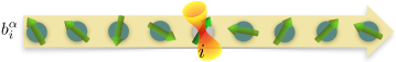
Figure 3: Alternative scheme to map out the local fields $b_{i}^{\alpha}$. A global pulse imposes the $XY$-$8$ pulse sequence on all spins and a focused pulse is in addition applied to spin $i$ to cancel the DD sequence on that single spin.

IV Pulse Errors

In the main text, we discussed different types of pulse errors. In our numerical simulation, we considered Systematic Amplitude pulse Error (SAE), Random Amplitude pulse Error (RAE) and Random Rotation axis Error (RRE). The fitting curves in Fig. 2 of the main text do not take into account of pulse errors. Here, we include the figures (Fig. 4) for the case with a $1\%$ RRE. We can see, for example in Fig. 4(a), that the frequency estimation is still very accurate while some measurement points may have a notable mismatch. We may also notice that the estimation of $b_{i}^{\alpha}$ is exceptionally robust to pulse errors since no pulse is applied to spin $i$ in the scheme. Other pulse errors have similar effects on the estimation of parameters.

Figure 4: (color online). Numerical simulation and curving fitting results with a Random Rotation axis Error (RRE) for each pulse. The RRE is of the form $e^{i\frac{\pi}{2}(\sigma^{\nu}+\alpha\sigma^{x}+\beta\sigma^{y}+\gamma\sigma^{z})}$ where $(\alpha,\beta,\gamma)$ is a vector with a random direction but fixed magnitude at $1\%$. (a)-(c) are used to retrieve $J_{79}^{xx}$, $J_{79}^{yy}$ and $J_{79}^{zz}$ between spins 7 and 9. (d) and (e) are used to extract $b_{6}^{x}$, $b_{6}^{y}$ and $b_{6}^{z}$ for spin 6. The blue solid lines are the best-fit lines with the simulated experimental data, and red dashed lines are the theoretical ones generated by the true Hamiltonian parameters. Other parameters are the same as in Fig. 2 of the main text.