Delay-Distortion-Power Trade Offs in Quasi-Stationary Source Transmission over Block Fading Channels

Abstract

This paper investigates delay-distortion-power trade offs in transmission of quasi-stationary sources over block fading channels by studying encoder and decoder buffering techniques to smooth out the source and channel variations. Four source and channel coding schemes that consider buffer and power constraints are presented to minimize the reconstructed source distortion. The first one is a high performance scheme, which benefits from optimized source and channel rate adaptation. In the second scheme, the channel coding rate is fixed and optimized along with transmission power with respect to channel and source variations; hence this scheme enjoys simplicity of implementation. The two last schemes have fixed transmission power with optimized adaptive or fixed channel coding rate. For all the proposed schemes, closed form solutions for mean distortion, optimized rate and power are provided and in the high SNR regime, the mean distortion exponent and the asymptotic mean power gains are derived. The proposed schemes with buffering exploit the diversity due to source and channel variations. Specifically, when the buffer size is limited, fixed channel rate adaptive power scheme outperforms an adaptive rate fixed power scheme. Furthermore, analytical and numerical results demonstrate that with limited buffer size, the system performance in terms of reconstructed signal SNR saturates as transmission power is increased, suggesting that appropriate buffer size selection is important to achieve a desired reconstruction quality.

I Introduction

Multimedia signals such as video exhibit quasi-stationary characteristics, causing the compression rate to vary over time. Wireless channels, on the other hand, also vary over time, making wireless video transmission challenging. In order to maintain a desired signal quality, multimedia communications over wireless channels involve buffering at the encoder and decoder to smooth out the source and channel variations at the cost of delay. For delay-constrained communications the buffer size is kept limited, and the transmitter controls the rate and/or transmission power to minimize the end-to-end distortion, while preventing buffer overflow and underflow. The goal of this paper is to study delay-distortion-power trade offs in transmission of quasi-stationary sources over block fading channels from the perspective of source and channel code design and the associated performance scaling laws.

There is a rich literature on source and channel coding for wireless channels. The end-to-end mean distortion for transmission of a stationary source over a block fading channel is considered in, e.g., [1]-[4], where the performance is studied in terms of the (mean) distortion exponent or the decay rate of the end-to-end mean distortion with (channel) signal to noise ratio (SNR) in the high SNR regime. Delay-limited communication of a stationary source over a wireless block fading channel from the channel outage perspective is studied in [5] and [6]. The transmission of a stationary source over a MIMO block fading channel with constant power transmission is considered in [7], where the distortion outage probability and the outage distortion exponent are considered as performance measures. Several schemes for transmission of a quasi-stationary source over a block fading channel are proposed in [8] to minimize the distortion outage probability. The results demonstrate the benefit of power adaption for delay-limited transmission of quasi-stationary sources over wireless block fading channels from a distortion outage perspective.

Considering delay-limited transmission of a quasi-stationary source over a wireless block fading channel and noting the buffer constraints, in this paper we propose a framework for rate and power adaptation that uses source and channel codes achieving the rate-distortion and the capacity in a given source and channel state. Throughout, we assume that the channel state information is known at the transmitter and the receiver. As described in Section II, the end-to-end mean distortion, the mean distortion exponent and asymptotic mean power gains are the performance metrics of interest. Under average transmission power and buffer size constraints, four designs are presented. The first scheme provides adaptation of source and channel coding rates and the transmission power such that the end-to-end mean distortion is minimized. The second scheme is a channel optimized power adaptation strategy to minimize the mean distortion for a given optimized fixed channel rate. This, for example, could be useful when we are interested in simple transmission schemes with a single channel (coding) rate. The other two designs are constant power delay-limited communication schemes with channel optimized adaptive or fixed rates.

The performance of the proposed schemes are evaluated and compared both analytically and numerically. The scaling laws involving mean distortion exponent and asymptotic mean power gain are derived in the large SNR regime with limited or asymptotic buffer sizes. The results demonstrate that the proposed schemes utilize the diversity provided by increasing the number of source blocks in a frame (buffer) at varying levels. Moreover, the presented schemes capture a larger (source) diversity gain when the non-stationary characteristic of the source is intensified or equivalently the variations in the source characteristics from one block to another increases. Another interesting observation is that with limited buffer size and increasing transmission power, the system performance in terms of reconstructed signal SNR saturates. In other words, depending on the level of source variations, delay constraint and the desired performance, the buffer size needs to be carefully designed to ensure the performance scales properly with transmission power. The results show that the proposed source and channel optimized rate and power adaptive scheme outperforms other proposed schemes in terms of the end-to-end mean distortion. For the case that the buffer constraint is relatively small in comparison to the power limit, it is seen that an adaptive power single channel rate scheme outperforms a rate adaptive scheme with constant transmission power. This is in contrast to the observation made in [9], which is from the Shannon capacity perspective.

Note that the delay-limited transmission in [1]-[8] refers to the scenario where each frame interval is short as it spans only a limited number of channel blocks and the transmitter cannot average out over channel fluctuations. Although we assume a quasi stationary source as in [8], we consider the end-to-end mean distortion and the buffer size limitation, and as such the resulting delay we investigate here is of a distinct nature and is primarily affected by the variability of the source statistics.

The paper is organized as follows. Following the description of system model in Section II, Section III presents the proposed scheme based on adaptive rate and power source and channel coding design to minimize mean distortion. Next, in Section IV, we present the scheme with adaptive power and fixed channel coding rate optimized for minimized mean distortion. Two constant power schemes are proposed in Section V. Performance comparisons and evaluations are presented in Sections VI and VII. Finally the paper is concluded in Section VIII.

II System Model

We consider the transmission of a quasi-stationary source over a block fading channel. The source is assumed to be independent identically distributed circularly symmetric complex Gaussian with zero mean and variance $\sigma^{2}_{s}$, $s\in\mathcal{S}=\{1,2,...,N_{s}\}$ in a given source block of $N$ samples [10]. The source state $s\in\mathcal{S}$ is a discrete random variable with the probability mass function (pmf) $p_{s}$. For optimized source coding rate $R_{s}$ bits per source sample in state $s$, the resulting distortion is $D=\sigma^{2}_{s}\,2^{-R_{s}}$ [11]. One frame of the source is defined as $K$ source blocks. We assume that the source sum rate in a frame is constrained to $\tilde{B}_{\rm{max}}$ bits per frame due to buffer (delay) limitations [12][13]. Therefore, we have $N{\sum_{j=1}^{K}R_{s_{j}}}\leq\tilde{B}_{\rm{max}}$, where ${s_{j}}$ is the source state in the source block $j$. Alternatively, we obtain

$$\frac{\sum_{j=1}^{K}R_{s_{j}}}{K}\leq B_{\rm{max}},$$ (1)

where $B_{\rm{max}}\overset{\Delta}{=}\frac{\tilde{B}_{\rm{max}}}{KN}$, and the LHS of (1) indicates the average source coding rate in bits per sample over a frame.

We consider a block fading channel for transmitting the source to the destination. Let $X$, $Y$ and $Z$, respectively indicate channel input, output and additive noise, where $Z$ is an i.i.d circularly symmetric complex Gaussian noise, $Z\sim\mathcal{CN}(0,1)$. Therefore, we have $Y=hX+Z$, where $h$ is the multiplicative fading. The channel gain $\alpha=|h|^{2}$ is assumed to be constant across one channel block and independently varies from one channel block to another according to the continuous probability density function $f(\alpha)$. For a Rayleigh fading channel, $\alpha$ is an exponentially distributed random variable, where we assume $E[\alpha]=1$. The instantaneous capacity of the fading Gaussian channel over one channel block (in bits per channel use) is given by $C(\alpha,\gamma)=\log_{2}(1+\alpha\gamma)$, where $\gamma$ is the transmission power. We consider the long term power constraint $\text{E}[\gamma]\leq\bar{P}$, where the expectation is taken over the fading distribution [5].

Each source frame is channel encoded to a single channel codeword spanning one channel block. The bandwidth expansion ratio of the system is denoted by $b$ channel uses per source sample, where $b\in{\mathcal{R}}^{+}\textbackslash(0,1)$. Thus, the source rates in a frame are assigned such that the following constraint is satisfied

$$\frac{\sum_{j=1}^{K}R_{s_{j}}}{K}=bR,$$ (2)

where $R$ in bits per channel use is the channel coding rate. Equations (1) and (2) result in $bR\leq B_{\rm{max}}.$ Assuming perfect knowledge at the transmitter and receiver of the source and channel states in a frame, $\gamma$, $R_{s_{j}}$ and $R$ can be generally chosen as a function of source and channel states, i.e., $\gamma=\gamma(\Sigma,\alpha)$, $R_{s_{j}}=R_{s_{j}}(\Sigma,\alpha)$ and $R=R(\Sigma,\alpha)$, where $\Sigma=[s_{1},...,s_{K}]$ is the vector of source states in a given frame. Thus, the end-to-end mean distortion in general is given by

$$\text{E}[D]=\text{E}_{\Sigma,\alpha}\left[\frac{\sum_{j=1}^{K}\sigma^{2}_{s_{j}}2^{-R_{s_{j}}}}{K}I(R\leq C(\alpha,\gamma))+\frac{\sum_{j=1}^{K}\sigma^{2}_{s_{j}}}{K}I(R>C(\alpha,\gamma))\right],$$ (3)

where $I$ is an indicator function which is $1$ when its argument is true and zero otherwise. Without loss of generality, we assume that $\sigma^{2}_{s_{1}},...,\sigma^{2}_{s_{K}}$ are in a descending order. Note that the problem and the proposed designs can be easily extended to the case in which one source frame corresponds to more than one fading channel blocks.

We define the buffer constrained mean distortion exponent, $\Delta^{B_{\rm{max}}}_{\textit{MD}}$, and the buffer unconstrained mean distortion exponent, $\Delta_{\textit{MD}}$ as our performance measures [1], where

$$\Delta^{B_{\rm{max}}}_{\textit{MD}}=\underset{\bar{P}\rightarrow\infty}{\lim}{-\frac{\ln{\text{E}[D]}}{\ln{\bar{P}}}},\;\;\;\;\;\Delta_{\textit{MD}}=\underset{\bar{P}\rightarrow\infty,{B_{\rm{max}}}\rightarrow\infty}{\lim}{-\frac{\ln{\text{E}[D]}}{\ln{\bar{P}}}}.$$ (4)

Let $\bar{P}_{1}$ and $\bar{P}_{2}$ be the average powers transmitted to asymptotically achieve a specific buffer constrained or unconstrained mean distortions by two different schemes. We define the corresponding asymptotic mean power gain as follows

$$G^{B_{\rm{max}}}_{M\!D}(\text{or }G_{M\!D})=10\log_{10}{\bar{P}_{2}}-10\log_{10}{\bar{P}_{1}}.$$ (5)

In the sequel, we also use the following mathematical definitions and approximations (see (5.1.53) of [14])

$$E_{p}(x):={\int^{\infty}_{1}}{\frac{e^{-x\alpha}}{\alpha^{p}}\mathrm{d}\alpha};\;\;\;\;\;\;E_{p}(0)=\frac{1}{p-1},\;p>1;\;\;\;\;\;\;\Gamma\left(t,x\right):=\int_{x}^{\infty}{\alpha^{t-1}e^{-\alpha}\mathrm{d}\alpha},\;\;x,t\geq 0$$ (6)

$$[x]^{+}:=\operatorname{\rm{max}}\{x,0\},\;\;\;\;\;\;E_{1}(x)\cong-E_{c}-\ln(x),\;\;\;\;\;\;\;\;\;e^{x}\cong 1+x\quad\text{if}\;x\rightarrow 0,$$ (7)

where $E_{c}=0.5772156649$ is the Euler constant. In the following sections, we explore designs to minimize the end-to-end mean distortion in the presence of average power and buffer constraints. The optimization variables are power $\gamma$ and rate $R$ in each channel block, and source rates $R_{s_{j}}$ in source block $j\in\{1,...,K\}$ over a frame, which may in general be a function of channel and source states. Depending on whether rate and/or power are adjusted or remain constant, we present four schemes in the sequel.

III Source and Channel optimized Rate and Power Adaptation

In this section, we consider power and rate adaptation with regard to source and channel states for improved performance of communication of a quasi-stationary source over a block fading channel. The objective is to devise power and rate adaptation strategies for each block of the channel and the source such that the end-to-end mean distortion is minimized, when the average power and buffer are respectively constrained to $\bar{P}$ and $B_{\rm{max}}$. The source and channel coding rates may be controlled with respect to the channel state to avoid channel outages such that $R\leq C(\alpha,\gamma)$. Thus, we have the following design problem.

Problem 1

The problem of delay-limited Source and Channel Optimized Rate and Power Adaptation (SCORPA) for communication of a quasi-stationary source with limited buffer over a block fading channel is formulated as follows

$$\underset{\gamma(\Sigma,\alpha),{R}_{s_{j}}(\Sigma,\alpha)}{\operatorname{min}}\;{\text{E}_{\Sigma,\alpha}\left[\sum_{j=1}^{K}\sigma^{2}_{s_{j}}2^{-R_{s_{j}}}\right]}\;\text{ subject to }$$ (8)

$$\text{E}[\gamma]\leq\bar{P},\;\;\;\;\;\;{\sum_{j=1}^{K}R_{s_{j}}}\leq KB_{\rm{max}}$$ (9)

$${\sum_{j=1}^{K}R_{s_{j}}}\leq{K}bC(\alpha,\gamma).$$ (10)

Proposition 1

Solution to Problem 1, denoted by $R^{*}_{s_{j}}$ and $\gamma^{*}$, for a given frame and an arbitrary block fading channel is given by

$$R^{*}_{s_{j}}=\begin{cases}0&\text{if}\;\alpha\leq\frac{\lambda}{bK\sigma_{s_{1}}^{2}}\\ \!\left[\log_{2}\frac{\sigma^{2}_{s_{j}}}{\lambda_{2}}\right]^{+}\!&\text{if}\;d_{1,m}\leq\alpha<d_{2,m},\;\alpha<c_{m}:\!\forall{m}\in\{1,...,K\}\\ \!\left[\log_{2}\frac{\sigma^{2}_{s_{j}}}{\mathbf{\tilde{\lambda}}_{2}}\right]^{+}\!&\text{if}\;\!d_{1,m}\leq\alpha<d_{2,m},\;\alpha\geq c_{m}:\forall{m}\in\{1,...,K\}\end{cases}$$ (11)

$$\gamma^{*}=\begin{cases}0&\text{if}\;\alpha\leq\frac{\lambda}{bK\sigma_{s_{1}}^{2}}\\ \frac{\frac{\alpha\lambda_{2}bK}{\lambda}-1}{\alpha}&\text{if}\;d_{1,m}\leq\alpha<d_{2,m},\;\alpha<c_{m}:\forall{m}\in\{1,...,K\}\\ \frac{2^{\frac{B_{\rm{max}}}{b}}-1}{\alpha}&\text{if}\;d_{1,m}\leq\alpha<d_{2,m},\;\alpha\geq c_{m}:\forall{m}\in\{1,...,K\},\end{cases}$$ (12)

where

$$c_{m}=2^{\frac{m+bK}{m}\frac{B_{\rm{max}}}{b}}\frac{\lambda}{bK\sqrt[m]{\sigma^{2}_{s_{1}}...\sigma^{2}_{s_{m}}}}$$ (13)

$$d_{1,m}=\frac{\lambda\sqrt[bK]{\sigma^{2}_{s_{1}}...\sigma^{2}_{s_{m}}}}{bK\sqrt[bK]{\sigma_{s_{m}}^{2(m+bK)}}}\;\;\;d_{2,m}=\begin{cases}\frac{\lambda\sqrt[bK]{\sigma^{2}_{s_{1}}...\sigma^{2}_{s_{m}}}}{bK\sqrt[bK]{\sigma_{s_{m+1}}^{2(m+bK)}}}&\text{if}\;m\neq K\\ \infty&\text{if}\;m=K\end{cases}$$ (14)

$$\lambda_{2}=\sqrt[m+bK]{\left(\sigma^{2}_{s_{1}}...\sigma^{2}_{s_{m}}\right)}\sqrt[m+bK]{(\frac{\lambda}{\alpha bK})^{bK}},\;\;\;\;\mathbf{\tilde{\lambda}}_{2}=\sqrt[n]{\frac{\sigma_{s_{1}}^{2}...\sigma^{2}_{s_{n}}}{2^{KB_{\rm{max}}}}}$$ (15)

$n$ is an integer in $\{1,...,K\}$ such that $\sigma_{s_{n+1}}^{2}<\mathbf{\tilde{\lambda}}_{2}\leq\sigma_{s_{n}}^{2}$. The parameter $\lambda$ is selected such that

$$\text{E}_{\Sigma}\!\left[\!\sum_{m=1}^{K}\!\int_{a_{1,m}}^{a_{2,m}}{\!\frac{2^{\frac{B_{\rm{max}}}{b}}-1}{\alpha}\!}f(\alpha)d\alpha\!\!+\!\!\!\int_{e_{1,m}}^{e_{2,m}}\!\!\left\{\!\sqrt[m+bK]{\sigma^{2}_{s_{1}}...\sigma^{2}_{s_{m}}}\!\!\sqrt[m+bK]{\left(\!\frac{bK}{\lambda}\!\right)^{m}}\!\alpha^{\frac{-bK}{m+bK}}\!-\!\alpha^{-1}\!\right\}f(\alpha)d\alpha\!\right]\!\!=\!\!\bar{P},$$ (16)

where

$$a_{1,m}\!=\!\max\{d_{1,m},c_{m}\},\;\;a_{2,m}\!=\!\max\{d_{2,m},c_{m}\},\;\;e_{1,m}\!=\!d_{1,m},\;\;e_{2,m}\!=\!\max\{\!\min\{c_{m},d_{2,m}\},e_{1,m}\!\}.$$ (17)

Specifically for Rayleigh block fading channel, (16) is simplified to

$$\text{E}_{\Sigma}\!\!\left[\!\sum_{m=1}^{K}(2^{\frac{B_{\rm{max}}}{b}}\!\!-\!\!1)(E_{1}(a_{1,m})\!\!-\!\!E_{1}(a_{2,m}))\!\!+\!\!\sqrt[m+bK]{\sigma^{2}_{s_{1}}...\sigma^{2}_{s_{m}}}\!\!\sqrt[m+bK]{\!\!\left(\frac{bK}{\lambda}\!\right)^{m}}\left(\!\Gamma\!\left(\frac{-bK}{m+bK}+1,e_{1,m}\!\right)\!\!-\!\!\right.\right.$$

$$\left.\left.\Gamma\left(\!\frac{-bK}{m+bK}+1,e_{2,m}\!\right)\!\right)\!+\!E_{1}(e_{2,m})\!-\!E_{1}(e_{1,m})\!\right]\!\!=\!\!\bar{P}$$ (18)

Remark 1

According to Proposition 1, if $\alpha\leq\frac{\lambda}{bK\sigma_{1}^{2}}$ (case 1 in (11) and (12)), channel transmission power and all the source rates in a given frame are set to zero. This corresponds to the scenario in which the channel gain and/or the variances of the source blocks within a frame are relatively small. Now suppose that $d_{1,m}\leq\alpha<d_{2,m}$, where $m\in\{1,...,K\}$ and $d_{1,m}$ and $d_{2,m}$ are functions of the source variances in states $\Sigma$. For $\alpha<c_{m}$ (case 2 in (11) and (12)), the available channel rate, which equals the channel capacity, is allocated to the $m$ source blocks with highest variances within the $K$ source blocks of the frame. For $\alpha\geq c_{m}$ (case 3 in (11) and (12)), due to the buffer size constraint, the channel coding rate is set to $B_{\rm{max}}/b$ and is allocated to the $n$ source blocks with highest variances within the $K$ source blocks of the frame, where $n$ is given in Proposition 1. Clearly, in case 2 the instantaneous channel capacity of the frame constrains the rate allocation to source blocks within the frame. In case 3, the buffer size constrains the rate allocation instead.

Proof:

The proof is provided in Appendix A. ∎

The next two propositions quantify the performance of the proposed SCORPA scheme in terms of the mean distortion and mean distortion exponent, respectively.

Proposition 2

Mean distortion obtained by SCORPA scheme for transmission of a quasi-stationary source over a Rayleigh block fading channel is given by

$$\text{E}[D]\!\!=\!\!\frac{1}{K}\text{E}_{\Sigma}\left[\sum_{j=1}^{K}\sigma^{2}_{s_{j}}\left(1\!-\!\exp(-{\frac{\lambda}{bK\sigma^{2}_{s_{1}}}})\right)\!\!+\!\!\sum_{m=1}^{K}\!\left(\!n\mathbf{\tilde{\lambda}}_{2}+\sum_{j=n+1}^{K}{\sigma^{2}_{s_{j}}}\!\right)\!\!\bigl{(}\exp(-a_{1,m})\!\!-\!\!\exp(-a_{2,m})\bigr{)}\!+\!\!\right.$$

$$\left.m\sqrt[m+bK]{\sigma^{2}_{s_{1}}...\sigma^{2}_{s_{m}}}\sqrt[m+bK]{\left(\frac{\lambda}{bK}\right)^{Kb}}\left(\Gamma(\frac{-bK}{m+bK}+1,e_{1,m})-\Gamma(\!\frac{-bK}{m+bK}+1,e_{2,m})\!\right)\!+\!\right.$$

$$\left.\sum_{j=m+1}^{K}\!\sigma^{2}_{s_{j}}\left(\exp(-e_{1,m})\!-\!\exp(-e_{2,m})\right)\right],$$ (19)

where $\lambda$, $\mathbf{\tilde{\lambda}}_{2}$, $n$, $a_{1,m}$, $a_{2,m}$, $e_{1,m}$ and $e_{2,m}$ are defined in Proposition 1.

Proof:

Considering exponentially distributed channel gain, using Proposition 1, (3)-(6), achieving (2) is straightforward. ∎

Proposition 3

For a Rayleigh block fading channel and with large power $\bar{P}$, SCORPA scheme achieves the mean distortion exponents $\Delta^{B_{\rm{max}}}_{\textit{MD}}=0$ and $\Delta_{\textit{MD}}=b$, respectively.

Proof:

We first consider the buffer constrained scenario. As evident from (16), we have $\lambda\rightarrow 0$ for large power constraint $\bar{P}\rightarrow\infty$. From (17), we obtain

$$e_{i,m}\rightarrow 0\;\;\;\forall{m}\in\{1,...,K-1\}\;\;\;i\in\{1,2\},\;\;\;\;\;\;\;e_{1,K}\rightarrow 0,\;\;\;\;\;\;\;e_{2,K}\rightarrow\infty.$$ (20)

Thus, noting (7), we have

$$E_{1}(e_{1,m})-E_{1}(e_{2,m})=-\ln(\frac{e_{1,m}}{e_{2,m}}),\;\;\;\forall{m}\in\{1,...,K-1\}$$ (21)

$$\Gamma\left(\frac{-bK}{m+bK}+1,e_{1,m}\right)-\Gamma\left(\frac{-bK}{m+bK}+1,e_{1,m}\right)=0,\;\;\;\forall{m}\in\{1,...,K-1\}$$ (22)

$$E_{1}(e_{1,K})-E_{1}(e_{2,K})=-\ln(e_{1,K})$$ (23)

$$\Gamma\left(\frac{-bK}{m+bK}+1,e_{1,K}\right)-\Gamma\left(\frac{-bK}{m+bK}+1,e_{2,K}\right)=\Gamma\left(\frac{-bK}{m+bK}+1,0\right).$$ (24)

From (17) it is observed that the equations similar to (20) to (24) are satisfied for $a_{1,m}$ and $a_{2,m}$. Hence, from (1) and by ignoring $\ln(\frac{bK}{\lambda})$ in contrast to $\frac{bK}{\lambda}$ for $\lambda\rightarrow 0$, we obtain

$$\text{E}_{\Sigma}\left[\sqrt[K+bK]{\sigma^{2}_{s_{1}}...\sigma^{2}_{s_{K}}}\sqrt[K+bK]{\left(\frac{bK}{\lambda}\right)^{K}}\Gamma\left(\frac{-bK}{K+bK}+1,0\right)\right]=\bar{P}.$$ (25)

Or equivalently $\sqrt[1+b]{\left(\frac{bK}{\lambda}\right)}\Gamma\left(\frac{1}{b+1},0\right)\text{E}_{\Sigma}\left[\sqrt[K+bK]{\sigma^{2}_{s_{1}}...\sigma^{2}_{s_{K}}}\right]=\bar{P}.$ Thus,

$$\sqrt[1+b]{\lambda}=\frac{\sqrt[1+b]{\left(bK\right)}\Gamma\left(\frac{1}{b+1},0\right)\text{E}_{\Sigma}\left[\sqrt[K+bK]{\sigma^{2}_{s_{1}}...\sigma^{2}_{s_{K}}}\right]}{\bar{P}}.$$ (26)

From (20) to (24) and noting $\lambda\rightarrow 0$, only the second term in (2) is non-negligible and therefore mean distortion is given by

$$\text{E}[D]=\frac{1}{K}\text{E}_{\Sigma}\left[n\mathbf{\tilde{\lambda}}_{2}+\sum_{j=n+1}^{K}{\sigma^{2}_{s_{j}}}\right]=\frac{1}{K}\text{E}_{\Sigma}\left[n\sqrt[n]{\frac{\sigma_{s_{1}}^{2}...\sigma^{2}_{s_{n}}}{2^{KB_{\rm{max}}}}}+\sum_{j=n+1}^{K}{\sigma^{2}_{s_{j}}}\right],$$ (27)

where $n$ is an integer in $\{1,2,...,K\}$ such that $\sigma^{2}_{s_{n+1}}<\sqrt[n]{\frac{\sigma_{s_{1}}^{2}...\sigma^{2}_{s_{n}}}{2^{KB_{\rm{max}}}}}\leq\sigma^{2}_{s_{n}}$. Therefore for any finite buffer constraint $B_{max}$, $\Delta_{\textit{MD}}^{B_{\rm{max}}}=0.$

We now consider the buffer unconstrained scenario. In this case we first let $B_{max}\rightarrow\infty$ in Propositions 1 and 2 and then increase the power $\bar{P}$. For $B_{\rm{max}}\rightarrow\infty$ and noting (13), we have $c_{m}\rightarrow\infty$. Thus, from (17), we obtain $a_{1,m}=a_{2,m}=c_{m}\rightarrow\infty$. Hence, the first term in (16) is omitted and for large power constraint $\lambda\rightarrow 0$. With $\lambda\rightarrow 0$, we still obtain (20) to (26). The second term in (2) is omitted and therefore, the mean distortion in (2) is simplified as

$$\text{E}[D]\!\!=\!\!\frac{1}{K}\text{E}_{\Sigma}\!\!\left[\!\!\sum_{j=1}^{K}\sigma^{2}_{s_{i}}\frac{\lambda}{bK\sigma^{2}_{s_{1}}}\!\!+\!\!K\sqrt[K+bK]{\sigma^{2}_{s_{1}}...\sigma^{2}_{s_{K}}}\sqrt[1+b]{\!\left(\frac{\lambda}{bK}\!\right)^{b}}\Gamma\!\left(\!\frac{1}{b+1},\!\right)\!\!+\!\!\sum_{m=1}^{K}\sum_{j=m+1}^{K}\!\sigma^{2}_{s_{i}}\!\left(d_{2,m}\!-\!d_{1,m}\right)\!\!\right]\!,$$

where noting $d_{1,m}$ and $d_{2,m}$ in (14), ignoring $\frac{\lambda}{bK}$ with respect to $\left(\frac{\lambda}{bK}\right)^{\frac{b}{b+1}}$ for $\lambda\rightarrow 0$ and utilizing (26) we have

$$\text{E}[D]=\frac{1}{\bar{P}^{b}}\left(\text{E}_{\Sigma}\left[\sqrt[K+bK]{\sigma^{2}_{s_{1}}...\sigma^{2}_{s_{K}}}\right]\right)^{b+1}\Gamma\left(\frac{1}{b+1},0\right)^{b+1}.$$ (28)

Therefore for any finite buffer constraint $B_{max}$, $\Delta_{\textit{MD}}=b$. Thus, the proof is complete. ∎

The performance of the proposed SCORPA scheme is studied in Section VII.

IV Channel Optimized Power Adaptation with Constant Channel Coding Rate

In this section, the aim is to find the optimized power allocation strategy and non-adaptive channel code rate $R$ such that the mean distortion for communication of a delay-limited quasi-stationary source over a block fading channel minimized. With a fixed channel rate, the channel code can be fixed, which simplifies the design and implementation of transceivers. Note that source coding rates in different blocks of a frame, $R_{s_{j}}$, may still be adapted. Also, we will find the best fixed channel coding rate $R$ to minimize the expected source distortion. The mean distortion in (3) for a fixed channel rate $R$ is simplified as follows

$$\text{E}[D]=\text{E}_{\Sigma}\left[\frac{\sum_{j=1}^{K}\sigma^{2}_{s_{j}}2^{-R_{s_{j}}}}{K}\right]\bigl{(}1-\text{Pr}\bigl{(}R>C\left(\alpha,\gamma\right)\bigr{)}\bigr{)}+\text{E}_{s}[\sigma_{s}^{2}]\text{Pr}\bigl{(}R>C\left(\alpha,\gamma\right)\bigr{)},$$ (29)

which is subject to the constraints in (1) and (2). We have the following design problem.

Problem 2

The problem of delay-limited Channel Optimized Power Adaptation with Constant Channel Rate (COPACR) for communication of a quasi-stationary source with limited buffer over a block fading channel is formulated as follows

$$\underset{\gamma(\Sigma,\alpha),R,R_{s_{j}}(\Sigma,\alpha)}{\operatorname{min}}\;\text{E}[D]\;\;\;\text{subject to}$$

$$\text{E}[\gamma]\leq\bar{P},\;\;\;\;\;\sum_{j=1}^{K}R_{s_{j}}=KbR,\;\;\;\;\;\;bR\leq B_{\rm{max}},$$ (30)

where $\text{E}[D]$ is given in (29).

The solution to Problem 2 is obtained in three steps. We may rewrite (29) as follows

$$\text{E}[D]=\text{Pr}\bigl{(}R>C\left(\alpha,\gamma\right)\bigr{)}\biggl{(}\text{E}_{s}[\sigma_{s}^{2}]-\text{E}_{\Sigma}\left[\frac{\sum_{j=1}^{K}\sigma^{2}_{s_{j}}2^{-R_{s_{j}}}}{K}\right]\biggr{)}+\text{E}_{\Sigma}\left[\frac{\sum_{j=1}^{K}\sigma^{2}_{s_{j}}2^{-R_{s_{j}}}}{K}\right].$$ (31)

For a given channel coding rate $R$, power adaptation only affects the mean distortion in (31) through the term $\text{Pr}\bigl{(}R>C\left(\alpha,\gamma\right)\bigr{)}$. Thus, the optimum $\gamma$ does not depend on $\Sigma$ (vector of source states). We first consider the design (sub)problem 3 below to find the optimized power adaptation strategy for a given $R$. Next, assuming a given $R$ and the resulting power adaptation strategy, noting (29), we consider another design (sub)problem 4 for source rate allocation to different blocks over a frame which aims at minimizing the term $\text{E}_{\Sigma}\left[{\sum_{j=1}^{K}\sigma^{2}_{s_{j}}2^{-R_{s_{j}}}}\right]$. As we shall see, the results of the two (sub)problems are derived in terms of $R$, which is then directly obtained by solving problem 2.

Problem 3 below formulates the power adaptation strategy for a given $R$. Note that

$$\text{E}_{\Sigma}\left[\frac{\sum_{j=1}^{K}\sigma^{2}_{s_{j}}2^{-R_{s_{j}}}}{K}\right]\leq\text{E}_{s}[\sigma_{s}^{2}],\;\forall R_{s_{j}}\geq 0.$$ (32)

Problem 3

With COPACR scheme and with a given channel coding rate $R$, the power adaptation problem is formulated as follows

$$\underset{\gamma}{\operatorname{min}}\;\text{Pr}(R>C(\alpha,\gamma))\;\text{subject to}\;\;\;\;\;\text{E}[\gamma]\leq\bar{P}{.}$$ (33)

Proposition 4

Solution to Problem 3 for optimized power adaptation over a block fading channel is given by

$$\gamma^{*}{(\alpha,R)}=\begin{cases}\frac{2^{R}-1}{\alpha}&\text{if}\;\;\alpha\geq\frac{2^{R}-1}{q^{*}_{1}(R)}\\ 0&\text{if}\;\;\alpha<\frac{2^{R}-1}{q^{*}_{1}(R)}{,}\end{cases}$$ (34)

in which $q^{*}_{1}(R)$ is selected such that the power constraint is satisfied with equality, i.e.,

$$\underset{\alpha\geq\frac{2^{R}-1}{q^{*}_{1}(R)}}{\int}{\frac{2^{R}-1}{\alpha}f(\alpha)\,\mathrm{d}\alpha}=\bar{P}.$$ (35)

Specifically for Rayleigh block fading channel, (35) is simplified to

$$\left(2^{R}-1\right)E_{1}\left(\frac{2^{R}-1}{q^{*}_{1}(R)}\right)=\bar{P}.$$ (36)

Proof:

The proof follows that of Proposition 4 in [5]. Based on (35), for Rayleigh block fading channel $q_{1}^{*}(R)$ is to satisfy (36). In fact $q_{1}^{*}(R)$ sets the SNR threshold below which the channel outage occurs. ∎

For a given channel coding rate $R$ and the optimized power adaptation strategy in Proposition 4, the outage probability $\bigl{(}R>C\left(\alpha,\gamma\right)\bigr{)}$ is fixed. Hence, minimizing mean distortion in (29) is equivalent to minimizing $\text{E}_{\Sigma}\left[{\sum_{j=1}^{K}\sigma^{2}_{s_{j}}2^{-R_{s_{j}}}}\right]$. This leads us to Problem 4 below which formulates the source rate allocation design for a given $R$ within the COPACR scheme.

Problem 4

For COPACR scheme with a given $R\leq\frac{B_{\rm{max}}}{b}$, the set of optimum source coding rates, $R^{*}_{s_{j}},j\in\{1,...,K\}$, is given by the solution to the following optimization problem

$$\begin{split}&\underset{R_{s_{j}}}{\operatorname{min}}\;\text{E}_{\Sigma}\left[{\sum_{j=1}^{K}\sigma^{2}_{s_{j}}2^{-R_{s_{j}}}}\right]\;\;\text{subject to: }\\ &\sum_{j=1}^{K}R_{s_{j}}=KbR,\;\;\;\;\;\;\;R_{s_{j}}\geq 0.\end{split}$$ (37)

Proposition 5

The solution to Problem 4 for an arbitrary block fading channel is given by

$$\begin{split}R^{*}_{s_{j}}=&\left[\log_{2}\frac{\sigma_{s_{j}}^{2}}{\lambda(R)}\right]^{+}\end{split}$$ (38)

with $\lambda(R)=\sqrt[n]{\frac{\sigma^{2}_{s_{1}}\times...\times\sigma^{2}_{s_{n}}}{2^{bKR}}},$ where $n$ is an integer in $\{1,2,...,K\}$ such that $\sigma^{2}_{s_{n+1}}<\lambda(R)\leq\sigma^{2}_{s_{n}}.$

Proof:

Using reverse water filling [11], the proof is straightforward. ∎

Now Proposition 6 below gives solution to Problem 2.

Proposition 6

The solution to Problem 2 for an arbitrary block fading channel is given by

$$\begin{split}R^{*}\!\!=\!\!\underset{R:\;0\leq bR\leq B_{\rm{max}}}{\operatorname{argmin}}\;\!\!\text{E}[D]\!\!=\!\!\text{E}_{s}[\sigma_{s}^{2}]\text{Pr}\biggl{(}\alpha<\frac{2^{R}-1}{q^{*}_{1}(R)}\biggr{)}\!\!+\!\!\biggl{(}\!1\!-\!\text{Pr}\biggl{(}\!\alpha<\frac{2^{R}-1}{q^{*}_{1}(R)}\!\biggr{)}\!\biggr{)}\text{E}_{\Sigma}\!\!\left[\!\frac{n\lambda(R)\!\!+\!\!\sum_{j=n+1}^{K}\sigma^{2}_{s_{j}}}{K}\!\right]\end{split}$$ (39)

with $q^{*}_{1}(R)$ satisfying (35) and $\lambda(R)$ given in Proposition 5. Consequently with the obtained $R^{*}$, $\gamma^{*}{(\alpha,R^{*})}$ and $R^{*}_{s_{j}}$ may be derived using Propositions 4 and 5, respectively.

Proof:

Using Propositions 4 and 5, we replace the optimized power adaptation and source rate allocation results into (29), which provides the mean distortion in terms of a single variable $R$. Hence, the optimized value of $R$ may be obtained numerically as indicated in (3). Thus, the proof is complete. Our extensive studies in the case of Rayleigh block fading channel reveals that the mean distortion in (39) is a convex function of $R$ and hence indicates a unique minimum at $R^{*}$. ∎

Proposition 7 below provides the mean distortion achieved by COPACR.

Proposition 7

For transmission of a quasi-stationary source over a Rayleigh block fading channel, the COPACR scheme achieves the mean distortion

$$\text{E}[D]=\text{E}_{s}[\sigma_{s}^{2}]\left(1-\exp(-\frac{2^{R^{*}}-1}{q^{*}_{1}(R^{*})})\right)+\exp\left(-\frac{2^{R^{*}}-1}{q^{*}_{1}(R^{*})}\right)\text{E}_{\Sigma}\left[\frac{n\lambda(R^{*})+\sum_{j=n+1}^{K}\sigma^{2}_{s_{j}}}{K}\right]$$ (40)

with $n$, $R^{*}$ and $\lambda(R^{*})$ in Proposition 5 and

$$\left(2^{R^{*}}-1\right)E_{1}\left(\frac{2^{R^{*}}-1}{q^{*}_{1}(R^{*})}\right)=\bar{P}.$$ (41)

Proof:

Using Proposition 6 for Rayleigh block fading channel, achieving (40) and (41) is straightforward. ∎

Proposition 8

For a Rayleigh block fading channel, the COPACR scheme achieves the mean distortion exponents $\Delta^{B_{\rm{max}}}_{\textit{MD}}=0$ and $\Delta_{\textit{MD}}=br_{1}$, where $r_{1}\in[0,1)$ denotes the COPACR buffer unconstrained multiplexing gain which can be calculated by numerically approximating $R^{*}$ as $R^{*}={r}_{1}\log_{2}\bar{P}+{r}_{0}$.

Proof:

The proof is provided in Appendix B. ∎

The performance of COPACR scheme is studied and compared in Section VII.

V Constant Power schemes

In this section, two constant power schemes for delay-limited transmission of a quasi-stationary source over a block fading channel with buffer and power limitations are considered. In the first scheme, the source and channel coding rates are adjusted based on the source or channel states to minimize the mean distortion; hence the scheme is labeled as Source and Channel Optimized Rate Adaptation with Constant Power (SCORACP). In the second scheme with Constant Rate and Constant Power (CRCP), the aim is to find the optimized fixed channel rate and adaptive source coding rates such that the mean distortion is minimized.

V-A Source and Channel Optimized Rate Adaptation with Constant Power

With SCORACP and constant transmission power $\bar{P}$, the instantaneous capacity is $C(\alpha)=\log_{2}{\left(1+\alpha\bar{P}\right)}$. As discussed, the source and channel coding rates may be controlled with respect to the channel state such that $R\leq C(\alpha)$. Thus, noting the buffer size constraint $B_{\rm{max}}$, we have the next design problem.

Problem 5

The problem of SCORACP for delay-limited communication of a quasi-stationary source with limited buffer over a block fading channel is formulated as follows for minimum mean distortion,

$$\underset{{R}_{sj}(\Sigma,\alpha)}{\operatorname{min}}\;{\text{E}_{\Sigma,\alpha}\left[{\sum_{j=1}^{K}\sigma^{2}_{s_{j}}2^{-R_{s_{j}}}}\right]}\;\;\text{ subject to}$$ (42)

$$\;{\sum_{j=1}^{K}R_{s_{j}}}\leq KB_{\rm{max}},\;\;\;\;\;{\sum_{j=1}^{K}R_{s_{j}}}\leq KbC(\alpha).$$ (43)

Proposition 9

Solution to Problem 5, denoted by $R^{*}_{s_{j}},j\in\{1,...,K\}$, for an arbitrary block fading channel is given by

$$\vspace{-8pt}R^{*}_{s_{j}}=\begin{cases}\left[\log_{2}\frac{\sigma_{s_{j}}^{2}}{\mathbf{\tilde{\lambda}}}\right]^{+}&\text{if}\;\alpha\geq c\\ \left[\log_{2}\frac{\sigma_{s_{j}}^{2}}{\lambda}\right]^{+}&\text{if}\;\alpha<c,\;\;\;d_{1,m}\leq\alpha<d_{2,m},\forall m\in{\{1,...,K\}},\end{cases}$$ (44)

where $\lambda=\sqrt[m]{\frac{\sigma_{s_{1}}^{2}...\sigma^{2}_{s_{m}}}{(1+\alpha\bar{P})^{bK}}},\;\mathbf{\tilde{\lambda}}=\sqrt[n]{\frac{\sigma_{s_{1}}^{2}...\sigma^{2}_{s_{n}}}{2^{KB_{\rm{max}}}}}$ and $n$ is an integer in $\{1,2,...,K\}$ such that $\sigma^{2}_{s_{n+1}}<\mathbf{\tilde{\lambda}}\leq\sigma^{2}_{s_{n}}$; and

$$d_{1,m}=\frac{\frac{\sqrt[bK]{\sigma^{2}_{s_{1}}...\sigma^{2}_{s_{m}}}}{(\sigma^{2}_{s_{m}})^{\frac{m}{bK}}}-1}{\bar{P}},\;\;\;\;\;d_{2,m}=\begin{cases}\frac{\frac{\sqrt[bK]{\sigma^{2}_{s_{1}}...\sigma^{2}_{s_{m}}}}{(\sigma^{2}_{s_{m+1}})^{\frac{m}{bK}}}-1}{\bar{P}}&\text{if}\;m\neq K\\ \infty&\text{if}\;m=K\end{cases},\;\;\;\;\;c=\frac{2^{\frac{B_{\rm{max}}}{b}}-1}{\bar{P}}.$$ (45)

Proof:

The proof is provided in Appendix C. ∎

The next two propositions quantify the mean distortion performance of SCORACP.

Proposition 10

The mean distortion obtained by SCORACP for transmission of a quasi-stationary source over a Rayleigh block fading channel is given by

$$\text{E}[D]=\frac{1}{K}\text{E}_{\Sigma}\left[\left(n\mathbf{\tilde{\lambda}}+\sum_{j=n+1}^{K}\sigma^{2}_{s_{j}}\right)\exp(-c)+\sum_{m=1}^{K}\left\{m\!\sqrt[m]{\sigma_{s_{1}}^{2}...\sigma^{2}_{s_{m}}}\bar{P}^{-1}\exp(\!\frac{1}{\bar{P}}\!)\right.\right.$$

$$\left.\left.\left((1+d_{1,m}\bar{P}\!)^{-\frac{bK}{m}+1}\!E_{\frac{bK}{m}}(\frac{1}{\bar{P}}+d_{1,m}\!)-(1+\min(d_{2,m},c)\bar{P})^{-\frac{bK}{m}+1}E_{\frac{bK}{m}}(\frac{1}{\bar{P}}+\min(d_{2,m},c))\right)+\right.\right.$$

$$\left.\left.\sum_{i=m+1}^{K}\!\sigma^{2}_{s_{i}}\left(\exp(-d_{1,m})-\exp(-\min(d_{2,m},c))\right)\right\}\right],$$ (46)

where $\mathbf{\tilde{\lambda}}$, $n$, $d_{1,m}$ and $d_{2,m}$ are defined in Proposition 9.

Proof:

Noting (3) and Proposition 9, we obtain

$$\text{E}[D]\!\!=\!\!\frac{1}{K}\text{E}_{\Sigma}\!\!\left[\!\!\int_{\alpha>c}\!\left(\!\!n\mathbf{\tilde{\lambda}}\!\!\!+\!\!\!\!\sum_{j=n+1}^{K}\sigma^{2}_{s_{j}}\!\!\right)f(\alpha)d\alpha\!\!+\!\sum_{m=1}^{K}\!\int_{\!\!\alpha\leq c,\;d_{1,m}\leq\alpha<d_{2,m}}\!\!\!\left(\!m\sqrt[m]{\frac{\sigma_{s_{1}}^{2}...\sigma^{2}_{s_{m}}}{\!(1\!+\!\!\alpha\bar{P}\!)^{bK}}}\!\!+\!\!\!\!\sum_{i=m+1}^{K}\!\sigma^{2}_{s_{i}}\!\right)\!f(\alpha)d\alpha\!\!\right]\!.$$ (47)

We change the variables as $u_{1}=\frac{1+\alpha\bar{P}}{\bar{P}}$ and $u_{2}=1+\alpha\bar{P}$, respectively for $\frac{bK}{m}=1$ and $\frac{bK}{m}>1$ in the second integral. Hence, noting the exponentially distributed channel gain and using (6), equation (47) is rewritten as (10). ∎

Proposition 11

For a Rayleigh block fading channel and with large power $\bar{P}$, the SCORACP scheme achieves the mean distortion exponents $\Delta^{B_{\rm{max}}}_{\textit{MD}}=0$ and $\Delta_{\textit{MD}}=1$

Proof:

We first consider the buffer constrained scenario. As denoted, it can intuitively be seen that $\Delta^{B_{\rm{max}}}_{\textit{MD}}$ of SCORACP is zero. However, because we need the mean distortion for large power constraint in Section VI we bring here the steps. For large power $\bar{P}\rightarrow\infty$ and from (45), we have

$$c\rightarrow 0,\;\;\;\;\;d_{1,m}\rightarrow 0\;\;\;\forall m\in\{1,...,K\},\;\;\;\;\;d_{2,m}\rightarrow\begin{cases}0&\forall m\in\{1,...,K-1\}\\ \infty&m=K.\end{cases}$$ (48)

Note that for $b>1$ and $m\in\{1,...,K\}$, $\frac{bK}{m}$ is greater than 1. Thus for $\bar{P}\rightarrow\infty$ and $b>1$, utilizing (7), we have

$$E_{\frac{bK}{m}}(\frac{1}{\bar{P}}+d_{1,m}\!)=\begin{cases}\frac{1}{\frac{bK}{m}-1}&m\in\{1,...,K-1\}\text{ and }b=1\\ E_{1}(\frac{1}{\bar{P}}+d_{1,m}\!)&m=K\text{ and }b=1\\ \frac{1}{\frac{bK}{m}-1}&b>1\end{cases}$$ (49)

and $\forall b>1$

$$E_{\frac{bK}{m}}(\frac{1}{\bar{P}}+d_{2,m})=\begin{cases}\frac{1}{\frac{bK}{m}-1}&\forall m\in\{1,...,K-1\}\\ 0&m=K.\end{cases}$$ (50)

Hence, from (10) we obtain

$$\text{E[D]}=\frac{1}{K}\text{E}_{\Sigma}\left(n\tilde{\lambda}+\sum_{j=n+1}^{K}\sigma^{2}_{s_{j}}\right)\exp(-c)+\bar{P}^{-1}V_{m},\;\;b>1,$$ (51)

where

$$V_{m}=\frac{1}{K}\text{E}_{\Sigma}\left[\sum_{m=1}^{K-1}\left\{m\!\sqrt[m]{\sigma_{s_{1}}^{2}...\sigma^{2}_{s_{m}}}\left((x_{1,m})^{-\frac{bK}{m}+1}-(x_{2,m})^{-\frac{bK}{m}+1}\right)\frac{1}{\frac{bK}{m}-1}\right.\right.$$

$$\left.\left.+\left(x_{2,m}-x_{1,m}\right)\sum_{i=m+1}^{K}\sigma^{2}_{s_{i}}\right\}+K\!\sqrt[K]{\sigma_{s_{1}}^{2}...\sigma^{2}_{s_{K}}}(x_{1,K})^{-b+1}\frac{1}{b-1}\right],$$ (52)

$$x_{i,m}=\frac{\sqrt[bK]{\sigma^{2}_{s_{1}}...\sigma^{2}_{s_{m}}}}{(\sigma^{2}_{s_{m+i-1}})^{\frac{m}{bK}}},\;i=\{1,2\},$$ (53)

and for $b=1$, we have

$$\text{E[D]}=\frac{1}{K}\text{E}_{\Sigma}\left(n\tilde{\lambda}+\sum_{j=n+1}^{K}\sigma^{2}_{s_{j}}\right)\exp(-c)+\bar{P}^{-1}W_{m},\;\;b=1,$$ (54)

where

$$W_{m}=\frac{1}{K}\text{E}_{\Sigma}\left[\sum_{m=1}^{K-1}\left\{m\!\sqrt[m]{\sigma_{s_{1}}^{2}...\sigma^{2}_{s_{m}}}\left((x_{1,m})^{-\frac{bK}{m}+1}-(x_{2,m})^{-\frac{bK}{m}+1}\right)\frac{1}{\frac{bK}{m}-1}\right.\right.$$

$$\left.\left.+\left(x_{2,m}-x_{1,m}\right)\sum_{i=m+1}^{K}\sigma^{2}_{s_{i}}\right\}+KE_{1}\left(\frac{x_{1,K}}{\bar{P}}\right)\sqrt[K]{\sigma_{s_{1}}^{2}...\sigma^{2}_{s_{K}}}\right].$$ (55)

Using (7), it is evident that the second term may be neglected with respect to the first term in both (51) and (54) for $\bar{P}\rightarrow\infty$ and limited buffer size; and therefore, we obtain

$$\text{E}[D]=\frac{1}{K}\text{E}_{\Sigma}\left[n\tilde{\lambda}+\sum_{j=n+1}^{K}{\sigma^{2}_{s_{j}}}\right]=\frac{1}{K}\text{E}_{\Sigma}\left[n\sqrt[n]{\frac{\sigma_{s_{1}}^{2}...\sigma^{2}_{s_{n}}}{2^{KB_{\rm{max}}}}}+\sum_{j=n+1}^{K}{\sigma^{2}_{s_{j}}}\right],$$ (56)

where $n$ is an integer in $\{1,2,...,K\}$ such that $\sigma^{2}_{s_{n+1}}<\sqrt[n]{\frac{\sigma_{s_{1}}^{2}...\sigma^{2}_{s_{n}}}{2^{KB_{\rm{max}}}}}\leq\sigma^{2}_{s_{n}}$. Therefore, $\Delta_{\textit{MD}}^{B_{\rm{max}}}=0.$

We now consider the buffer unconstrained scenario. Obviously from (45), we have $c\rightarrow\infty$. However, we still have (48) to (V-A) and the first term in (51) and (54) is zero. Therefore, using (7) in (51) and (54), we derive $\Delta_{\textit{MD}}=\underset{\bar{P}\rightarrow\infty}{\lim}-\frac{\ln{\text{E}[D]}}{\ln{\bar{P}}}=1.$ Thus, the proof is complete. ∎

V-B Constant Channel Rate with Constant Power

With CRCP scheme, the fixed channel rate and adaptive source coding rates are optimized to minimize the mean distortion when the power is constant. The following three propositions express the optimized rate, mean distortion and mean distortion exponent obtained by CRCP.

Proposition 12

For delay-limited transmission of a quasi-stationary source over a block fading channel using the CRCP scheme and limited buffer, the optimum rates $R^{*}$ and $R^{*}_{s_{j}},\;j\in\{1,...,K\}$ for minimum mean distortion are obtained as follows,

$$R^{*}= \underset{R:\;0\leq bR\leq B_{\rm{max}}}{\operatorname{argmin}}\!\!\!\text{E}[D]\!\!=\!\!\text{E}_{s}[\sigma_{s}^{2}]\text{Pr}\biggl{(}\!\alpha\!\!<\!\!\frac{2^{R}-1}{\bar{P}}\!\biggr{)}\!\!+\!\!\biggl{(}1\!\!-\!\!\text{Pr}\biggl{(}\alpha<\frac{2^{R}-1}{\bar{P}}\biggr{)}\biggr{)}\!\text{E}_{\Sigma}\!\left[\!\!\frac{n\lambda(R)\!+\!\sum_{j=n+1}^{K}\sigma^{2}_{s_{j}}}{K}\!\!\right]\!,$$ (57)

$$R^{*}_{s_{j}}= \left[\!\!\log_{2}\frac{\sigma_{s_{j}}^{2}}{\lambda(R^{*})}\right]^{+},\text{ where}\;\;\;\lambda(R)=\sqrt[n]{\frac{\sigma^{2}_{s_{1}}\times...\times\sigma^{2}_{s_{n}}}{2^{bKR}}},$$ (58)

$n$ is an integer in $\{1,...,K\}$ such that $\sigma_{s_{i}}^{2}\geq{\lambda}$ for $i\leq n$ and $\sigma^{2}_{s_{i}}<{\lambda}$ for $i>n;\;i\in\{1,...,K\}$.

Proof:

Since the power is constant, the channel capacity and the mean distortion respectively are given as $C(\alpha)=\log_{2}(1+\alpha\bar{P})$ and

$$\text{E}[D]=\text{E}_{s}[\sigma_{s}^{2}]\text{Pr}\biggl{(}\alpha<\frac{2^{R}-1}{\bar{P}}\biggr{)}+\text{E}_{\Sigma}\left[{\sum_{j=1}^{K}\sigma^{2}_{s_{j}}2^{-R_{s_{j}}}}\right]\biggl{(}1-\text{Pr}\biggl{(}\alpha<\frac{2^{R}-1}{\bar{P}}\biggr{)}\biggr{)}.$$ (59)

For a given channel coding rate $R$, minimizing mean distortion in (59) is equivalent to minimizing $\text{E}_{\Sigma}\left[{\sum_{j=1}^{K}\sigma^{2}_{s_{j}}2^{-R_{s_{j}}}}\right]$. As noted, using reverse water filling, this leads us to Problem 4 and Proposition 5 which provides the source rate allocation for a given $R$. Hence, the optimized value of $R$ may be obtained numerically as indicated in (57). Thus, the proof is complete. ∎

Proposition 13

For transmission of a quasi-stationary source over a Rayleigh block fading channel, the CRCP scheme achieves the mean distortion

$$\text{E}[D]=\text{E}[\sigma^{2}]\left(1-\exp(\frac{2^{R^{*}}-1}{\bar{P}})\right)+\exp(\frac{2^{R^{*}}-1}{\bar{P}})\text{E}_{\Sigma}\left[\frac{n\lambda(R^{*})+\sum_{j=n+1}^{K}\sigma^{2}_{j}}{K}\right]$$ (60)

with $n$, $R^{*}$ and $\lambda(R^{*})$ in Proposition 12, and the mean distortion exponents $\Delta^{B_{\rm{max}}}_{\textit{MD}}=0$ and $\Delta_{\textit{MD}}=1-\tilde{r}_{1}$, where $\tilde{r}_{1}=\frac{1}{b+1}$ denotes the CRCP buffer unconstrained multiplexing gain.

Proof:

The proof is provided in Appendix D. ∎

Note that although the approach used in the proof of Proposition 13 is similar to that in [4], the source considered in [4] is stationary.

VI Analytical Performance Comparison

In the sequel, we quantify the respective asymptotic mean power gains $G^{B_{\rm{max}}}_{\textit{MD}}$ and $G_{\textit{MD}}$ of SCORPA, COPACR, SCORACP and CRCP for transmission of a quasi-stationary source over a block fading channel. As observed from equations (81), (27), (56) and (90) for large power and with buffer constraints, all schemes provide the same mean distortion independent of the power constraint. Since $\Delta^{B_{\rm{max}}}_{\textit{MD}}=0$, there is no meaningful $G^{B_{\rm{max}}}_{M\!D}$. Thus in the following we only address $G_{\textit{MD}}$ and $\Delta_{\textit{MD}}$.

Proposition 14

In transmission of a quasi-stationary source over a Rayleigh block fading channel, the asymptotic mean power gains obtained by SCORPA with respect to COPACR, $G_{M\!D,1}$, COPACR with respect to SCORACP, $G_{M\!D,2}$, and CRCP with respect to SCORACP, $G_{M\!D,3}$, are given by

$$G_{M\!D,1}=\frac{10}{b}\log_{10}{\frac{\text{E}_{\Sigma}[\sqrt[K]{\sigma_{s_{1}}^{2}\times...\times\sigma_{s_{K}}^{2}}]\bar{P}_{2}^{b(1-r_{1})}2^{-br_{0}}}{(\Gamma(\frac{1}{b+1},0))^{b+1}(\text{E}_{\Sigma}[\sqrt[K+bK]{\sigma_{s_{1}}^{2}\times...\times\sigma_{s_{K}}^{2}}])^{b+1}}},$$ (61)

$$G_{M\!D,2}=\begin{cases}\frac{10}{r_{1}}\log_{10}\frac{W_{m}}{\text{E}_{\Sigma}[\sqrt[K]{\sigma_{s_{1}}^{2}\times...\times\sigma_{s_{K}}^{2}}]\bar{P}_{2}^{1-r_{1}}2^{-r_{0}}}&b=1\\ \frac{10}{br_{1}}\log_{10}{\frac{V_{m}}{\text{E}_{\Sigma}[\sqrt[K]{\sigma_{s_{1}}^{2}\times...\times\sigma_{s_{K}}^{2}}]\bar{P}_{2}^{1-br_{1}}2^{-br_{0}}}}&b>1\end{cases}$$ (62)

and

$$G_{M\!D,3}=\begin{cases}20\log_{10}\!{\frac{W_{m}\bar{P}_{2}^{\frac{-1}{2}}}{\left(2^{-\tilde{r}_{0}}\text{E}_{\Sigma}\left[\sqrt[K]{\sigma^{2}_{s_{1}}\times...\times\sigma^{2}_{s_{K}}}\right]+2^{\tilde{r}_{0}}\text{E}_{s}[\sigma_{s}^{2}]\right)}},&b=1\\ \frac{b+1}{b}10\log_{10}\!{\frac{V_{m}\bar{P}_{2}^{\frac{-1}{b+1}}}{\left(2^{-b\tilde{r}_{0}}\text{E}_{\Sigma}\left[\sqrt[K]{\sigma^{2}_{s_{1}}\times...\times\sigma^{2}_{s_{K}}}\right]+2^{\tilde{r}_{0}}\text{E}_{s}[\sigma_{s}^{2}]\right)}},&b>1,\end{cases}$$ (63)

where $r_{0}$ and $r_{1}$ are given in Proposition 8, $\tilde{r}_{0}$ is defined in Proposition 13, $V_{m}$ and $W_{m}$ are respectively given in (V-A) and (V-A); and $\bar{P}_{2}$ is the power limit in scheme 2 (see Table I or II).

Proof:

The proof is provided in Appendix E. ∎

For large power constraint $\bar{P}_{2}$, (61)-(63) is simplified as follows

$$G_{M\!D,1}=(1-r_{1})10\log_{10}{\bar{P}_{2}},\;\;\;\;G_{M\!D,2}=\frac{(br_{1}-1)}{br_{1}}10\log_{10}{\bar{P}_{2}},\;\;\;\;G_{M\!D,3}=\frac{-1}{b}10\log_{10}{\bar{P}_{2}}.$$ (64)

As evident, $G_{\textit{MD}}$ depends on the power constraint and bandwidth expansion ratio. One sees that both $G_{M\!D,1}$ and, $G_{M\!D,2}$ for $br_{1}>1$ are increasing functions of the power. On the other hand $G_{M\!D,3}$ is negative and is a decreasing function of the power.

Tables I and II present the value of $G_{M\!D}$ for two relatively large values of ${\bar{P}_{2}}$. One sees that, an adaptive power scheme with constant channel rate performs better than an adaptive channel rate scheme with constant power from mean distortion perspective if $br_{1}>1$. As such, if we wish to control only one parameter (power or rate) for efficient transmission in the presence of source and channel variations, adapting power leads to a superior mean distortion performance. Nonetheless, adapting rate still provides performance gain.

The mean distortion exponent $\Delta_{\textit{MD}}$ of the presented schemes which are derived in line with the proofs of the Propositions 8, 3, 11 and 13 are expressed in Table III. The mean distortion exponent indicates the speed at which the mean distortion ($\rm dB$) reduces as the average power (limit) ($\rm dB$) increases. Therefore, as evident, this speed improves as bandwidth expansion ratio $b$ increases with SCORPA, COPACR and CRCP schemes, while it is fixed to 1 with SCORACP. Furthermore, the $\Delta_{\textit{MD}}$ obtained by all proposed schemes is independent of the average power limit $\bar{P}$. It is noteworthy that for $b=1$, $\Delta_{\textit{MD}}$ of COPACR is lower than that of SCORACP, while this is reverse for $br_{1}>1$, where $r_{1}$ denotes the COPACR buffer unconstrained multiplexing gain. Thus, it is evident that for large power constraint and $br_{1}>1$ with buffer unconstrained scenario, the adaptive power scheme with optimized fixed channel rate outperforms the adaptive rate with fixed power design scheme from mean distortion exponent aspect. The results in Tables I to III indicate that from the perspective of mean distortion, for delay-limited communication of quasi-stationary sources, CRCP scheme may not be an appropriate design.

TABLE I: Asymptotic mean power gain $G_{M\!D}$ of scheme 1 with respect to scheme 2 for source U defined in Section VII, unlimited buffer size, $K=2$ and $\bar{P}_{2}=40\rm dB$, where $\bar{P}_{2}$ is the power limit for the scheme 2.

$G_{M\!D}$	Scheme 1	Scheme 2	$b=1$	$b=2$	$b=4$	$b=6$
$G_{M\!D,1}$	SCORPA	COPACR	$5.27$	$5.74$	$6.02$	$6.10$
$G_{M\!D,2}$	COPACR	SCORACP	$-0.008$	$9.78$	$17.46$	$19.93$
$G_{M\!D,3}$	CRCP	SCORACP	$-28.34$	$-24.97$	$-19.45$	$-17.67$

TABLE II: Asymptotic mean power gain $G_{M\!D}$ of scheme 1 with respect to scheme 2 for source U defined in Section VII, unlimited buffer size, $K=2$ and $\bar{P}_{2}=45\rm dB$, where $\bar{P}_{2}$ is the power limit for the scheme 2.

$G_{M\!D}$	Scheme 1	Scheme 2	$b=1$	$b=2$	$b=4$	$b=6$
$G_{M\!D,1}$	SCORPA	COPACR	$5.84$	$6.39$	$6.76$	$6.87$
$G_{M\!D,2}$	COPACR	SCORACP	$-0.05$	$11.91$	$21.00$	$23.95$
$G_{M\!D,3}$	CRCP	SCORACP	$-32.27$	$-27.47$	$-20.71$	$-18.50$

TABLE III: Mean distortion exponent $\Delta_{\textit{MD}}$ of the proposed schemes for source U.

Scheme	SCORPA	COPACR	SCORACP	CRCP
$\Delta_{\textit{MD}}$	$b$	$br_{1}$	1	$\frac{b}{b+1}$

VII Performance evaluation

In this section, the performance of the proposed schemes are compared through numerical computations and evaluated for different source variances and frame sizes. To this end, we consider Rayleigh fading channel and two quasi-stationary sources with $N_{s}=9$ where the variance of the source in the state $s$ is $\sigma^{2}_{s}(s)=(1+(s-1)^{2}):\forall{s}\in\{1,...,N_{S}\}$. For the first source, labeled as U, the probability of being in different states is considered uniform which results in $\text{E}_{s}[\sigma_{s}^{2}]=23.66$. For the second source, G, the said distribution follows a discrete Gaussian distribution with a mean $5.49$ and a variance $2.52$ so as to have $\text{E}_{s}[\sigma_{s}^{2}]=23.66$. We also consider a stationary source D with $\sigma^{2}_{s}=23.66$, which is obviously equal to $\text{E}_{s}[\sigma_{s}^{2}]$, same as expected variances of U and G. For fair comparisons, we assume that $\tilde{B}_{\rm{max}}$ increases linearly with $K$ such that $B_{\rm{max}}$ is independent of $K$.

Fig. 1 depicts reconstructed SNR (RSNR) performance of the presented schemes defined as $10\log_{10}\frac{\text{E}_{s}[\sigma^{2}_{s}]}{\text{E}[D]}$ with respect to the power constraint $\bar{P}$ for different values of $K$. As observed, RSNR improves as the source changes faster. In fact, the delay due to buffering of the source blocks in a frame allows us to use source diversity. However, the speed of this improvement decreases as $K$ increases. Our simulations for the quasi-stationary source U indicate that buffering of more than $K=4$ blocks does not provide additional performance improvements.

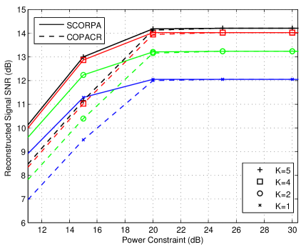
(a)

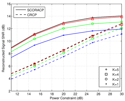
(b)

Figure 1: RSNR of (a) SCORPA and COPACR schemes (b) SCORACP and CRCP schemes, versus power constraint for different $K$, $B_{\rm{max}}=4$ and $b=1$.

Figs. 2 and 3 demonstrate the RSNR performance of the proposed schemes for bandwidth expansion ratios $b=1$ and $b=2$. As noted in Section VI, for $b=1$ and large $B_{\rm{max}}$, here $B_{\rm{max}}=20$, SCORACP outperforms COPACR. This is while for $b>1$ or limited $B_{\rm{max}}$, COPACR outperforms SCORACP for large enough power constraint. A larger bandwidth expansion ratio, $b$, corresponds to larger number of channel uses per source sample and hence, as the results confirm, leads to improved RSNR performance.

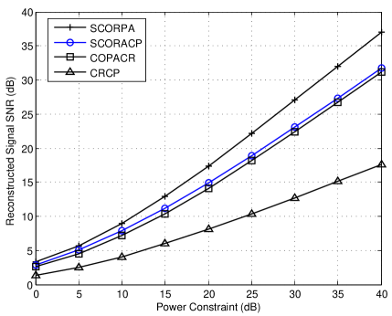
(a)

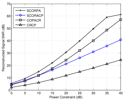
(b)

Figure 2: RSNR versus power constraint for $K=2$, $B_{\rm{max}}=20$ and (a) $b=1$ (b) $b=2$.

As observed in Fig. 2, the proposed SCORPA scheme achieves an asymptotic mean power gain of about $\rm 5.81\,dB$ and $\rm 5.91\,dB$ with respect to COPACR, for $\bar{P}=\rm 40\,dB$ and $b=1$ and $b=2$, respectively. In the same settings, the COPACR scheme achieves asymptotic mean power gains of about $\rm\,-0.60dB$ and $9.39\rm\,dB$ with respect to SCORACP; and CRCP achieves gains of $\rm\,-28.7dB$ and $\rm-25.22\,dB$ with respect to SCORACP. Note that $\bar{P}$ is the power limit for the second scheme in each comparison. The results obtained from simulations and what is reported in Table I from analyses match reasonably well given the assumption of high average SNR considered in the analytical performance evaluations.

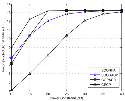
(a)

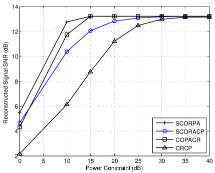
(b)

Figure 3: RSNR versus power constraint for $K=2$, $B_{\rm{max}}=4$ and (a) $b=1$ (b) $b=2$.

Figs. 2 and 3 also demonstrate the effect of $B_{\rm{max}}$. As observed, a given frame (buffer) size, $B_{\rm{max}}$, imposes a certain RSNR cap on the performance. As power limit, $\bar{P}$, increases, the RSNR improves until it saturates at this RSNR cap and any further increase of power will not help with RSNR performance. This confirms the substantial impact of buffer size on the performance. In the unsaturated regime, the performance and the speed by which it improves with respect to the power naturally depends on the system parameters and the rate and power allocation strategy. As evident in (81), (27), (56) and (90), the value of the RSNR cap depends on the source statistics, $K$, and $B_{\rm{max}}$ and is independent of the rate and power allocation strategy.

Fig. 4 demonstrates the RSNR performance of the presented schemes for different sources. The results show that a larger source diversity may be exploited as the non-stationary characteristics of the source intensifies (from source D to U), and therefore RNR increases in general. This is not only evident in the RSNR level at which the performance statures (for large power constraints), it is also visible in the unsaturated RSNR regime (low to medium transmission power). Moreover, one sees that the relative performance gains explained from using the proposed rate and/or power adaptation strategies are attainable in the unsaturated regime disregarding the source characteristics.

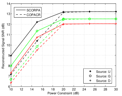
(a)

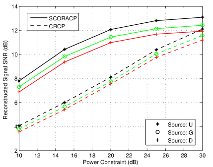
(b)

Figure 4: RSNR of (a) SCORPA and COPACR schemes (b) SCORACP and CRCP schemes, versus power constraint for three different sources, $K=2$, $B_{\rm{max}}=4$ and $b=1$.

VIII Conclusions

In this paper, we have considered delay-distortion-power trade-offs in transmission of a quasi-stationary source over a block fading channel when the buffer size is limited. Aiming at minimizing the mean distortion, we have introduced two optimized power transmission strategies as well as two other design schemes with constant transmission power. In the high SNR regime, we have derived different scaling laws involving mean distortion exponent and asymptotic mean power gain. The analyses of the presented schemes indicate that the buffer limit particularly affects the performance as the average transmission power increases; and as such needs to be carefully taken into account in the design. The proposed schemes with buffering exploit the diversity gain due to non-stationary characteristics of the source and channel variations to different levels. Our studies confirm the benefit of power adaption along with rate adaptation from a mean distortion perspective and for delay-limited transmission of quasi-stationary sources with limited buffer over wireless block fading channels.

Future research in this direction could investigate the potential dependency of different source blocks in the design. Also, it is interesting to model the characteristics of practical multimedia coding standards within the proposed framework and hence quantify the potential achievable performance gains. From a theoretical perspective, one could also consider a multiuser setting and explore design paradigms exploiting source and channel variations (diversity) in a multiuser setting.

Appendix A Proof of Proposition 1

Considering the power and buffer size constraints and equation (2), it is necessary to set the power such that $bC(\alpha,\gamma)\leq B_{\rm{max}}$. Thus, we may use the following constraint

$$bC(\alpha,\gamma)\leq B_{\rm{max}}$$ (65)

instead of the third constraint in Problem 1.

Due to the fact that in Problem 1, the objective and the constraints are convex functions of $\gamma$ and $R_{s_{j}}$, we take a Lagrange optimization approach. Hence, using $C(\alpha,\gamma)=\log_{2}(1+\alpha\gamma)$, Problem 1 may be restated as follows

$$\underset{\gamma,{R}_{s_{j}}}{\operatorname{min}}\;\biggl{\{}\text{E}_{\Sigma,\alpha}\left[\sum_{j=1}^{K}\sigma^{2}_{s_{j}}2^{-R_{s_{j}}}\right]+\lambda E[\gamma]+\lambda_{0}b\log_{2}(1+\alpha\gamma)+\lambda_{1}\left(\sum_{j=1}^{K}{R_{s_{j}}}-Kb\log_{2}(1+\alpha\gamma)\right)\biggr{\}}.$$ (66)

Differentiating (66) with respect to $R_{s_{j}}$ and $\gamma$, setting them to zero and noting the fact that $R_{s_{j}}$ and $\gamma$ are to be nonnegative, we obtain

$$R_{s_{j}}=\left[\log_{2}{\frac{\sigma^{2}_{s_{j}}}{\lambda_{2}}}\right]^{+}\;\;\;\forall j\in\{1,...,K\}$$ (67)

$$\gamma=\left[\frac{\frac{\alpha\lambda_{3}bK}{\lambda}-1}{\alpha}\right]^{+},$$ (68)

where $\lambda_{2}=\frac{\lambda_{1}}{\ln 2}$ and $\lambda_{3}=\lambda_{2}-\frac{\lambda_{0}}{K\ln 2}$.

Here, we continue to solve the problem in different cases when the constraint (65) is active or inactive. Obviously, when the constraint is inactive, i.e.,

$$bC(\alpha,\gamma)<B_{\rm{max}}$$ (69)

and $\lambda_{0}=0$, we have $\lambda_{3}=\lambda_{2}$. Alternatively, noting (68) and (69), the constraint (65) is inactive if

$$\frac{\alpha\lambda_{2}bK}{\lambda}<2^{\frac{B_{\rm{max}}}{b}}.$$ (70)

From (68) it is seen that $\gamma=0$ if $\frac{\alpha\lambda_{2}bK}{\lambda}\leq 1$ or equivalently, $\lambda_{2}\leq\frac{\lambda}{\alpha bK}.$ Considering the forth constraint in Problem 1, $R_{s_{j}}=0$ for $\gamma=0$. Noting (67), $R_{s_{j}}=0,\forall{j}\in\{1,...K\}$ if ${\lambda_{2}}\geq\sigma^{2}_{s_{1}}$. Hence, the power and the rate are set to zero if $\frac{\lambda}{bK\sigma^{2}_{s_{1}}}\geq\alpha$. Now assume

$$\sigma^{2}_{s_{m+1}}<\lambda_{2}\leq\sigma^{2}_{s_{m}}.$$ (71)

As evident from (67), the rate is allocated to the $m$ blocks out of $K$ blocks. From (10), (67) and (68), we have $\frac{\sigma^{2}_{s_{1}}...\sigma^{2}_{s_{m}}}{\lambda_{2}^{m}}=\left(\frac{\alpha\lambda_{2}bK}{\lambda}\right)^{bK}$ and therefore,

$$\lambda_{2}=\sqrt[m+bK]{\left(\sigma^{2}_{s_{1}}...\sigma^{2}_{s_{m}}\right)}\sqrt[m+bK]{\left(\frac{\lambda}{\alpha bK}\right)^{bK}}.$$ (72)

Noting (71), we obtain

$$\sigma^{2}_{s_{m+1}}<\lambda_{2}=\sqrt[m+bK]{\sigma^{2}_{s_{1}}...\sigma^{2}_{s_{m}}}\sqrt[m+bK]{\left(\frac{\lambda}{\alpha bK}\right)^{bK}}\leq\sigma^{2}_{s_{m}},$$ (73)

which indicates $d_{1,m}\!=\!\frac{\!\lambda\sqrt[bK]{\sigma^{2}_{s_{1}}...\sigma^{2}_{s_{m}}}\!}{bK\!\sqrt[bK]{{\sigma_{s_{m}}}^{2(m+bK)}}}\!\leq\!\alpha<d_{2,m}\!=\!\frac{\!\lambda\sqrt[bK]{\sigma^{2}_{1}...\sigma^{2}_{{s_{m}}}}\!}{bK\!\sqrt[bK]{{\sigma_{s_{m+1}}}^{2(m+bK)}}}.$ Obviously $d_{2,K}=\infty$. Given the value of $\lambda_{2}$ computed in (72), (70) may be rewritten as follows

$$\alpha<c_{m}=2^{\frac{m+bK}{m}\frac{B_{\rm{max}}}{b}}\frac{\lambda}{bK\sqrt[m]{\sigma^{2}_{s_{1}}...\sigma^{2}_{s_{m}}}}.$$ (74)

Now assume the constraint (65) is active, i.e.,

$$bC(\alpha,\gamma)=B_{\rm{max}},$$ (75)

$\lambda_{0}\neq 0$ and $\alpha\geq c_{m}$. Equivalently $\frac{\alpha\lambda_{3}bK}{\lambda}=2^{\frac{B_{\rm{max}}}{b}}.$ Therefore, utilizing (67), (68) and (75), $\gamma$ and $R_{s_{j}}$ are given by

$$\gamma=\left[\frac{2^{\frac{B_{\rm{max}}}{b}}-1}{\alpha}\right]^{+}\;\;\;\;\text{if}\;\;\;\alpha\geq c_{m}$$ (76)

and

$$R_{s_{j}}=\left[\log_{2}{\frac{\sigma^{2}_{s_{j}}}{{\lambda}_{2}}}\right]^{+}\;\;\;\forall j\in\{1,...,K\}.$$ (77)

Consider $\sigma^{2}_{s_{n+1}}<{\lambda}_{2}\leq\sigma^{2}_{s_{n}}$. As observed from (77), the rate is allocated to the $n$ blocks out of $K$ blocks. Therefore, from (10), (76) and (77), we obtain $\frac{\sigma^{2}_{s_{1}}...\sigma^{2}_{s_{n}}}{{\lambda}_{2}^{n}}=2^{KB_{\rm{max}}}.$ Hence, ${\lambda}_{2}$ is obtained as follows

$${\lambda}_{2}=\sqrt[n]{\frac{\sigma_{s_{1}}^{2}...\sigma^{2}_{s_{n}}}{2^{KB_{\rm{max}}}}}\;\;\;\;\text{if}\;\;\;\alpha\geq c_{m}.$$ (78)

To distinguish between $\lambda_{2}$ in the two cases described, i.e., in (72) and (78), we replace it with the new multiplier $\mathbf{\tilde{\lambda}}_{2}$ in (77) to (78), when describing the Proposition 1.

The parameter $\lambda$ is set to satisfy the power constraint $\text{E}[\gamma]=\bar{P}$. Thus, (16) is derived. Noting exponentially distributed channel gain, we can obtain (1) and therefore the proof is complete.

Appendix B Proof of Proposition 8

We first consider COPACR with the buffer constrained scenario. Since the buffer constrained mean distortion exponent, $\Delta^{B_{\rm{max}}}_{\textit{MD}}$, of SCORPA is zero, we expect that that $\Delta^{B_{\rm{max}}}_{\textit{MD}}$ of the other proposed schemes are also equal to zero. However, we need to compute the mean for large power constraint. Therefore, in the following we write the mathematically steps to obtain $\Delta^{B_{\rm{max}}}_{\textit{MD}}$. Due $\Delta^{B_{\rm{max}}}_{\textit{MD}}$. Due to the fact that $R^{*}$ is (41) for large power $\bar{P}\rightarrow\infty$, we have $\left(\frac{2^{R^{*}}-1}{q^{*}_{1}(R^{*})}\right)\rightarrow 0$. Now using (7) in (41), we obtain

$$\frac{2^{R^{*}}-1}{q^{*}_{1}(R^{*})}=\exp\left(\frac{-\bar{P}}{2^{R^{*}}-1}\right).$$ (79)

From (7) and (79), mean distortion in (40) is given by

$$\text{E}[D]=\text{E}_{s}[\sigma_{s}^{2}]\exp\left(\frac{-\bar{P}}{2^{R^{*}}-1}\right)+\text{E}_{\Sigma}\left[\frac{n\lambda(R^{*})+\sum_{j=n+1}^{K}\sigma^{2}_{s_{j}}}{K}\right].$$ (80)

As evident, for large power the second term in (80) is dominant and therefore, in order to minimize $\text{E}[D]$ in (80), it is necessary to set $R^{*}=\frac{B_{\rm{max}}}{b}$, we have

$$\text{E}[D]=\text{E}_{\Sigma}\left[\frac{n\lambda(\frac{B_{\rm{max}}}{b})+\sum_{j=n+1}^{K}\sigma^{2}_{s_{j}}}{K}\right]=\frac{1}{K}\text{E}_{\Sigma}\left[n\sqrt[n]{\frac{\sigma_{s_{1}}^{2}...\sigma^{2}_{s_{n}}}{2^{KB_{\rm{max}}}}}+\sum_{j=n+1}^{K}{\sigma^{2}_{s_{j}}}\right],$$ (81)

where $n$ is an integer in $\{1,2,...,K\}$, such that $\sigma^{2}_{s_{n+1}}<\sqrt[n]{\frac{\sigma_{s_{1}}^{2}...\sigma^{2}_{s_{n}}}{2^{KB_{\rm{max}}}}}\leq\sigma^{2}_{s_{n}}$ and hence $\Delta^{B_{\rm{max}}}_{\textit{MD}}=\underset{\bar{P}\rightarrow\infty}{\lim}{-\frac{\ln{\text{E}[D]}}{\ln{\bar{P}}}}=0.$

Next, we consider the buffer unconstrained scenario. For large $\bar{P}$ and $B_{\rm{max}}$, it is expected that $R$ is large enough for limited source variances and from Proposition 5, $\lambda(R)$ is very small. Thus, $n$ is set to $K$ and we have

$$\lambda(R)=\sqrt[K]{\sigma^{2}_{s_{1}}\times...\times\sigma^{2}_{s_{K}}}2^{-bR}.$$ (82)

Replacing (82) into (40), the mean distortion is given by

$$\text{E}[D]=\text{E}_{s}[\sigma_{s}^{2}]\left(1-\exp(-\frac{2^{R^{*}}-1}{q^{*}_{1}(R^{*})})\right)+\exp\left(-\frac{2^{R^{*}}-1}{q^{*}_{1}(R^{*})}\right)\text{E}_{\Sigma}\left[\sqrt[K]{\sigma^{2}_{s_{1}}\times...\times\sigma^{2}_{s_{K}}}\right]2^{-bR^{*}}.$$ (83)

In order for $\text{E}[D]$ to tend to zero, it is necessary that $\frac{2^{R^{*}}-1}{q^{*}_{1}(R^{*})}\rightarrow 0$. Note that $2^{-bR^{*}}$ tends to zero for large $R^{*}$ and power. Now similar to the buffer constrained scenario, (79) is obtained. Thus, noting (7) and (79), the mean distortion in (83) is given by

$$\text{E}[D]=\text{E}_{s}[\sigma_{s}^{2}]\exp\left(\frac{-\bar{P}}{2^{R^{*}}-1}\right)+\text{E}_{\Sigma}\left[\sqrt[K]{\sigma^{2}_{s_{1}}\times...\times\sigma^{2}_{s_{K}}}\right]2^{-bR^{*}}.$$ (84)

Hence, $R^{*}$ is to be chosen such that $\text{E}[D]$ given in (84) is minimized. As stated, $R^{*}$ is a function of the bandwidth expansion ratio $b$, the power constraint $\bar{P}$ and the source variances in different blocks of a given frame. Fig. 5 demonstrates $R^{*}$ in bits per channel use as a function of $\bar{P}$ for different bandwidth expansion ratios $b$ and exponentially distributed channel gain. It is evident that $R^{*}$ changes linearly with $\log_{2}\bar{P}$ for large $\bar{P}$, given $b$ and the source variances. Thus, $R^{*}$ may be described by

$$R^{*}={r}_{1}\log_{2}\bar{P}+{r}_{0},$$ (85)

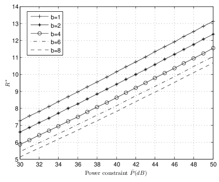
Figure 5: $R^{*}$ versus $\bar{P}$(dB) in COPACR scheme for different bandwidth expansion ratios $b$ over a block Rayleigh fading channel and source U.

where ${r}_{1}$ and ${r}_{0}$ are obtained by least square fitting as shown in Table IV(a). Note that the results in Fig. 1 are due to the quasi-stationary Gaussian source U described in Section VII and additive Gaussian channel noise $\mathcal{N}(0,1)$. Nonetheless, based on our experiments changing the source or the Gaussian noise statistics merely reflects in the fitting parameters $r_{0}$ and $r_{1}$ and do not affect the linear shape of the curves. The parameter $r_{1}$ is referred to as the buffer unconstrained multiplexing gain. From (84) and (85), we have

$$\text{E}[D]=\text{E}_{s}[\sigma_{s}^{2}]\exp\left(\frac{-\bar{P}}{2^{r_{0}}\bar{P}^{r_{1}}-1}\right)+\text{E}_{\Sigma}\left[\sqrt[K]{\sigma^{2}_{s_{1}}\times...\times\sigma^{2}_{s_{K}}}\right]2^{-br_{0}}\bar{P}^{-br_{1}}.$$ (86)

As evident, to have $\text{E}[D]\rightarrow 0$ for large power, it is necessary that the power exponent in the first and second terms to be respectively less than 1 and more than zero. Thus, $r_{1}\in[0,1)$, and therefore we can ignore the first term with respect to the second to obtain

$$\text{E}[D]=\text{E}_{\Sigma}\left[\sqrt[K]{\sigma^{2}_{1}\times...\times\sigma^{2}_{K}}\right]\bar{P}^{-br_{1}}2^{-br_{0}}.$$ (87)

Thus, $\Delta_{\textit{MD}}=\underset{\bar{P}\rightarrow\infty}{\lim}{-\frac{\ln{\text{E}[D]}}{\ln{\bar{P}}}}=br_{1}.$

TABLE IV: Parameters (a) $r_{0}$ and $r_{1}$ in COPACR scheme (b) $\tilde{r}_{1}$ and $\tilde{r}_{0}$ in CRCP scheme, for source U described in Section VII with the buffer unconstrained scenario and $K=2$ as a function of bandwidth expansion ratio $b$.

$b$	$r_{1}$	$r_{0}$
$1$	$0.90$	$-1.83$
$2$	$0.89$	$-2.39$
$4$	$0.88$	$-3.03$
$6$	$0.87$	$-3.41$
$8$	$0.86$	$-3.68$

(a)

$b$	$\tilde{r}_{1}$	$\tilde{r}_{0}$
1	0.50	-0.19
2	0.33	0.20
4	0.20	0.32
6	0.14	0.31
8	0.11	0.29

(b)

Appendix C Proof of Proposition 9

We solve the problem in two different cases 1) $B_{\rm{max}}\leq bC(\alpha)$ and 2) $B_{\rm{max}}>bC(\alpha)$, where in case 1 and 2, respectively the first and the second constraints in (43) have to be satisfied. Cases 1 and 2 respectively are equivalent to $\alpha\geq\frac{2^{B_{\rm{max}}}-1}{\bar{P}}$ and $\alpha<\frac{2^{B_{\rm{max}}}-1}{\bar{P}}$.

Therefore, using Lagrange optimization approach, we have

$$J={\text{E}_{\Sigma,\alpha}\left[\frac{\sum_{j=1}^{K}\sigma^{2}_{s}2^{-2R_{s_{j}}}}{K}\right]}+\lambda_{1}\sum_{j=1}^{K}{R_{s_{j}}}.$$ (88)

Differentiating $J$ with respect to $R_{s_{j}}$, setting it to zero and noting the fact that $R_{s_{j}}$ is to be nonnegative, we obtain

$$R_{s_{j}}=\left[\log_{2}\frac{\sigma_{s_{j}}^{2}}{\lambda}\right]^{+},$$ (89)

where $\lambda=\frac{\lambda_{1}}{2\ln 2}$. Satisfying the first constraint in (43) in the case $B_{\rm{max}}\leq C(\alpha)$ imposes $\lambda=\sqrt[n]{\frac{\sigma_{s_{1}}^{2}...\sigma^{2}_{s_{n}}}{2^{KB_{\rm{max}}}}}$, where $n$ is an integer in $\{1,2,...,K\}$ such that $\sigma^{2}_{s_{n+1}}<\lambda\leq\sigma^{2}_{s_{n}}.$

Noting (43) and (89) in the case $B_{\rm{max}}>C(\alpha)$, we obtain $\lambda=\sqrt[m]{\frac{\sigma_{s_{1}}^{2}...\sigma^{2}_{s_{m}}}{(1+\alpha\bar{P})^{bK}}},$ where $m$ is an integer in $\{1,2,...,K\}$ such that $\sigma^{2}_{s_{m+1}}<\lambda\leq\sigma^{2}_{s_{m}}.$ Thus, we have $d_{1,m}=\frac{\frac{\sqrt[bK]{\sigma^{2}_{s_{1}}...\sigma^{2}_{s_{m}}}}{(\sigma^{2}_{s_{m}})^{\frac{m}{bK}}}-1}{\bar{P}}\leq\alpha<d_{2,m}=\frac{\frac{\sqrt[bK]{\sigma^{2}_{s_{1}}...\sigma^{2}_{s_{m}}}}{(\sigma^{2}_{s_{m+1}})^{\frac{m}{bK}}}-1}{\bar{P}},$ where $d_{2,K}=\infty$.

To distinguish between $\lambda$ in the two cases described, we replace it with the new multiplier $\mathbf{\tilde{\lambda}}$ in case 1, when describing the Proposition 9.

Appendix D Proof of Proposition 13

Using E[D] in (57) for Rayleigh block fading channel with the given optimized $R^{*}$, achieving (60) is straightforward. For $\bar{P}\rightarrow\infty$ with the buffer constrained scenario, the solution to (58), $R^{*}$, have to be set to $\frac{B_{\rm{max}}}{b}$. Therefore, noting (58) and (60) we obtain

$$\text{E}[D] =\frac{1}{K}\text{E}_{\Sigma}\left[n\sqrt[n]{\frac{\sigma_{s_{1}}^{2}...\sigma^{2}_{s_{n}}}{2^{KB_{\rm{max}}}}}+\sum_{j=n+1}^{K}{\sigma^{2}_{s_{j}}}\right],$$ (90)

where $n$ is an integer in $\{1,2,...,K\}$ such that $\sigma^{2}_{s_{n+1}}<\sqrt[n]{\frac{\sigma_{s_{1}}^{2}...\sigma^{2}_{s_{n}}}{2^{KB_{\rm{max}}}}}\leq\sigma^{2}_{s_{n}}.$ Therefore, $\Delta_{\textit{MD}}^{B_{\rm{max}}}=0.$

For $\bar{P}\rightarrow\infty$ and $B_{\rm{max}}\rightarrow\infty$ with bounded source variances, it is expected that $R^{*}$ is large. Thus using reverse water-filling, the rate is allocated to all blocks in a given frame, i.e., $n=K$, and we obtain $\lambda(R^{*})=\sqrt[K]{\sigma^{2}_{s_{1}}\times...\times\sigma^{2}_{s_{K}}}2^{-bR^{*}}$. Replacing $\lambda(R^{*})$ into (60), the mean distortion is rewritten as follows $\text{E}[D]=\text{E}_{s}[\sigma_{s}^{2}]\left(1-\exp(\frac{2^{R^{*}}-1}{\bar{P}})\right)+\exp(\frac{2^{R^{*}}-1}{\bar{P}})\text{E}_{\Sigma}\left[\sqrt[K]{\sigma^{2}_{s_{1}}\times...\times\sigma^{2}_{s_{K}}}\right]2^{-bR^{*}}.$ Note the fact that for large $R^{*}$, we have $2^{-2bR^{*}}=0$. Therefore, in order for $\text{E}[D]$ to tend to zero for large power, it is necessary to have $\frac{2^{R^{*}}-1}{\bar{P}}\rightarrow 0$. Thus, using (7), we have

$$\text{E}[D] =\text{E}_{s}[\sigma_{s}^{2}]\frac{2^{R^{*}}-1}{\bar{P}}+\text{E}_{\Sigma}\left[(\sigma^{2}_{s_{1}}\times...\times\sigma^{2}_{s_{K}})^{\frac{1}{K}}\right]2^{-bR^{*}}.$$ (91)

We seek $R^{*}$ such that E[D] is minimized. Fig. 6 demonstrates $R^{*}$ in bits per channel use as a function of $\bar{P}$ for different bandwidth expansion ratios $b$ and exponentially distributed channel gain. The results are for source $U$ described in Section VII, however, our experiments with other sources reveal curves of similar behavior. It is evident that $R^{*}$ changes linearly with $\log_{2}\bar{P}$ for large $\bar{P}$, given $b$ and source variances. Thus, $R^{*}$ may be described by

$$R^{*}=\tilde{r}_{1}\log_{2}\bar{P}+\tilde{r}_{0}.$$ (92)

Figure 6: $R^{*}$ versus $\bar{P}$(dB) in CRCP scheme for different bandwidth expansion ratios $b$ over a block Rayleigh fading channel and source U.

The parameter $\tilde{r}_{1}$ denotes the CRCP buffer unconstrained multiplexing gain. From (90) and (92), we obtain $\text{E}[D]\!\!=\!\!\text{E}_{s}[\sigma_{s}^{2}]{\bar{P}^{\tilde{r}_{1}-1}2^{\tilde{r}_{0}}}\!\!+\!\!\text{E}_{\Sigma}\left[\sqrt[K]{\sigma^{2}_{s_{1}}\times...\times\sigma^{2}_{s_{K}}}\right]\bar{P}^{-b\tilde{r}_{1}}2^{-b\tilde{r}_{0}}.$ When $\bar{P}\rightarrow\infty$, for $\text{E}[D]\rightarrow 0$ we need to have $\tilde{r}_{1}\in[0\;1)$. Changing $\tilde{r}_{1}$ from 0 to 1, the power exponents ${\tilde{r}_{1}-1}$ and ${-b\tilde{r}_{1}}$ vary from $-1$ to $0$ and $0$ to $-b$, respectively. For large power constraint and a given value of $\tilde{r}_{1}$, one of the two terms $\bar{P}^{\tilde{r}_{1}-1}$ or $\bar{P}^{-b\tilde{r}_{1}}$ with the larger exponent dominates. As the two exponents vary in opposite directions when $\tilde{r}_{1}$ changes, the minimum value of the dominating exponent occurs where the two exponents are equal. As a result for maximum mean distortion exponent, we should have

$$\tilde{r}_{1}=\frac{1}{(b+1)}.$$ (93)

Thus, we obtain $\text{E}[D]\!\!=\!\!\bar{P}^{-\frac{b}{b+1}}\biggl{(}2^{-b\tilde{r}_{0}}\text{E}_{\Sigma}\left[\!\!\sqrt[K]{\sigma^{2}_{s_{1}}\times...\times\sigma^{2}_{s_{K}}}\right]+2^{\tilde{r}_{0}}\text{E}_{s}[\sigma_{s}^{2}]\biggr{)}$ and $\Delta_{\textit{MD}}\!\!=\!\!\underset{\bar{P}\rightarrow\infty}{\lim}\!{-\frac{\ln{\text{E}[D]}}{\ln{\bar{P}}}}\!\!=\!\!\frac{b}{b+1}.$ Table IV(b) demonstrate $\tilde{r}_{0}$ and $\tilde{r}_{1}$ obtained by least squared fitting of the results in Fig. 6 to the model in equation (92). As evident, the results coincide with the analytical solution presented in (93).

Appendix E Proof of Proposition 14

The average power to asymptotically achieve a certain mean distortion using SCORPA and COPACR schemes are denoted by $\bar{P}_{1}$ and $\bar{P}_{2}$, respectively. Thus, we can use (5) to derive $G\!_{M\!D}$.

Noting (28) and (87), we set

$$\vspace{-2pt}\frac{1}{\bar{P}_{1}^{b}}\left(\text{E}_{\Sigma}\left[\sqrt[K+bK]{\sigma^{2}_{1}...\sigma^{2}_{K}}\right]\right)^{b+1}\Gamma\left(\frac{1}{b+1},0\right)^{b+1}=\text{E}_{\Sigma}\left[\sqrt[K]{\sigma^{2}_{1}\times...\times\sigma^{2}_{K}}\right]\bar{P}_{2}^{-br_{1}}2^{-br_{0}}.$$ (94)

Therefore, we can derive (61). Achieving (62) or (63) is straightforward, when we use (87), (51) and (54) or (51), (54) and (86); and obtain the following

$$\text{E}_{\Sigma}\left[\sqrt[K]{\sigma^{2}_{1}\times...\times\sigma^{2}_{K}}\right]\bar{P}_{1}^{-br_{1}}2^{-br_{0}}=\bar{P}_{2}^{-1}V_{m},\;\;b>1$$ (95)

and

$$\text{E}_{\Sigma}\left[\sqrt[K]{\sigma^{2}_{1}\times...\times\sigma^{2}_{K}}\right]\bar{P}_{1}^{-br_{1}}2^{-br_{0}}=\bar{P}_{2}^{-1}W_{m},\;\;b=1$$ (96)

or

$$\bar{P}_{1}^{-\frac{b}{b+1}}\biggl{(}2^{-b\tilde{r}_{0}}\text{E}_{\Sigma}\left[\sqrt[K]{\sigma^{2}_{1}\times...\times\sigma^{2}_{K}}\right]+2^{\tilde{r}_{0}}\text{E}[\sigma^{2}]\biggr{)}=\bar{P}_{2}^{-1}V_{m},\;\;b>1,$$ (97)

and

$$\bar{P}_{1}^{-\frac{1}{2}}\biggl{(}2^{-\tilde{r}_{0}}\text{E}_{\Sigma}\left[\sqrt[K]{\sigma^{2}_{1}\times...\times\sigma^{2}_{K}}\right]+2^{\tilde{r}_{0}}\text{E}[\sigma^{2}]\biggr{)}=\bar{P}_{2}^{-1}W_{m},\;\;b=1.$$ (98)

References

• [1] J. N. Laneman, G. W. Wornell, and J. G. Apostolopoulos, “Source-channel diversity for parallel channels,” IEEE Trans. Inf. Theory, vol. 51, pp. 3518–3539, Oct. 2005.
• [2] D. Gunduz and E. Erkip, “Joint source-channel codes for MIMO block-fading channels,” IEEE Trans. Inf. Theory, vol. 54, pp. 116–134, Jan. 2008.
• [3] K. Bhattad, K. R. Narayanan, and G. Caire, “On the distortion SNR exponent of some layered transmission schemes,” IEEE Trans. Inf. Theory, vol. 54, pp. 2943–2958, July 2008.
• [4] B. Dunn and J. Laneman, “Characterizing source-channel diversity approaches beyond the distortion exponent,” in Allerton Conf. Commun. Control and Computing, (Monticello IL, USA), Sept. 2005.
• [5] G. Caire, G. Taricco, and E. Biglieri, “Optimum power control over fading channels,” IEEE Trans. Inf. Theory, vol. 45, pp. 1468–1489, July 1999.
• [6] V. Hanly and D. Tse, “Multiaccess fading channels. Part II: Delay-limited capacities,” IEEE Trans. Inf. Theory, vol. 44, pp. 2816–2831, Nov. 1998.
• [7] L. Peng and A. Guillen i Fabregas, “Distortion outage probability in MIMO block-fading channels,” in IEEE Int. Symp. Inform. Theory, (Austin, Texas, U.S.A), pp. 2223–2227, June 2010.
• [8] R. Joda and F. Lahouti, “Delay-limited source and channel coding of quasi-stationary sources over block fading channels: design and scaling laws,” IEEE Trans. Commun., vol. 61, pp. 1562–1572, Apr. 2013.
• [9] M. Alouini and A. Goldsmith, “Capacity of Rayleigh fading channels under different adaptive transmission and diversity-combining techniques,” IEEE Trans. Veh. Technol., vol. 48, pp. 1165–1181, July 1996.
• [10] Z. He, Y. Liang, L. Chen, I. Ahmad, and D. Wu, “Power-rate-distortion analysis for wireless video communication under energy constraints,” IEEE Trans. Circuits Syst. Video Technol., vol. 15, pp. 1468–1489, May 2005.
• [11] T. M. Cover and J. A. Thomas, Elements of Information Theory. New York: Wiley, 1991.
• [12] Y. Sun and I. Ahmad, “A robust and adaptive rate control algorithm for object-based video coding,” IEEE Trans. Circuits Syst. Video Technol., vol. 14, pp. 1167–1182, Oct. 2004.
• [13] W. Ding, “Joint encoder and channel rate control of VBR video over ATM networks,” IEEE Trans. Circuits Syst. Video Technol., vol. 7, pp. 266–278, Apr. 1997.
• [14] M. Abramowitz and I. A. Stegun, Handbook of Mathematical Functions. June 1974.