Ultrashort pulses in an inhomogeneously broadened two-level medium: Soliton formation and inelastic collisions

Abstract

Using numerical simulations, we study propagation of ultrashort light pulses in an inhomogeneously broadened two-level medium. There are two main issues in our study. The first one concerns the transient process of self-induced transparency soliton formation, in particularly the compression of the pulse which seems to be more effective in the case of homogeneous broadening. The second question deals with the collisions of counter-propagating solitons. It is shown that the level of inhomogeneous broadening has substantial effect on elasticity of such collisions.

1 Introduction

Self-induced transparency (SIT) is one of the basic phenomena of nonlinear optics. This effect resulting in formation of temporal solitons (so-called $2\pi$ pulses) in a resonantly absorbing medium was described in the pioneering papers by McCall and Hahn [1, 2]. There is an extensive literature on this topic including the classic monograph by Allen and Eberly [3] and a number of reviews (see [4, 5, 6, 7], to name a few). The continuing study of SIT is motivated by the fundamental and general character of the two-level model which is the basic tool for explanation of this phenomenon. The investigation of the properties of this model based on the semiclassical Maxwell-Bloch equations is necessary for our understanding of the nature of light-matter interaction. There is a number of generalizations, as well, aiming to take into account the near-dipole-dipole interactions (local-field correction) in the dense resonant media [8], Stark shift of the absorption line [9], and few-cycle pulse dynamics in the regime of invalidity of the rotating-wave approximation [10, 11]. Using the two-level model and its generalizations, the broad spectrum of SIT studies was performed including invariant pulse propagation and optical switching in dense media [12, 13], quasiadiabatic following analysis [14], incoherent solitons [15], SIT soliton lasers [16], SIT soliton collisions [17, 18], SIT in Bragg reflectors and photonic crystals [19, 20, 21], coherent pulse propagation and SIT effects in doped waveguides and amplifiers [22, 23], SIT in the presence of Kerr nonlinearity [24, 25], etc.

The aim of this paper is to consider some details of SIT soliton formation and interaction between solitons in the two-level medium with inhomogeneous broadening of resonant line. This broadening is due to the fact that, generally, the frequency of resonant transition is not the same for all atoms of the medium. The importance of inhomogeneous broadening can be illustrated by the example of the so-called area theorem. This theorem governs the change of the “area” $S(z)=(2\mu/\hbar)\int A(z,t)dt$ of the pulse propagating in the medium and can be written in the form

$$\tan\frac{S(z)}{2}=\tan\frac{S_{0}}{2}\exp\left(-\frac{\alpha z}{2}\right),$$ (1)

where $\mu$ is the component of transition dipole moment parallel to the polarization vector of the electric field, $A$ the electric field amplitude, $S_{0}$ the initial area, $\alpha$ the absorption coefficient of the medium, $\hbar$ the Planck constant. It is known that the area theorem (1) is strictly valid only for the inhomogeneously broadened media, though the main features of SIT can be observed in the case of homogeneous broadening as well [6]. This was confirmed recently by Yu et al. [26] who performed the direct simulations of area change. They demonstrated that in the case of homogeneous broadening, approach of the area to the stationary value corresponding to the SIT soliton is accompanied by slowly damping oscillations. These oscillations cannot be described by the standard formulae such as (1).

The present paper continues previous studies of inhomogeneously broadened media in comparison to their homogeneously broadened counterparts. Our attention is directed to the two questions studied in our recent works [18, 27] in the approximation of homogeneous broadening, viz. the transient process of SIT soliton formation and the collisions of such solitons. After Sec. 2 where the model is described, we discuss these two questions in Sec. 3 and 4, respectively. The paper closes with the brief conclusions of the results obtained.

2 Problem statement

Light interaction with the two-level medium at every spatial point is governed by the system of semiclassical Bloch equations for population difference $W$ and microscopic polarization $R$:

$$\frac{dR}{d\tau} = i\Omega W+iR\delta-\gamma_{2}R,$$ (2)

$$\frac{dW}{d\tau} = 2i(\Omega^{*}R-R^{*}\Omega)-\gamma_{1}(W-1),$$ (3)

where $\Omega=(\mu/\hbar\omega)A$ is the normalized electric field amplitude (or dimensionless Rabi frequency), and $\gamma_{1}=(\omega T_{1})^{-1}$ and $\gamma_{2}=(\omega T_{2})^{-1}$ are the rates of longitudinal and transverse relaxation, respectively. Since we are interested in consideration of the inhomogeneously broadened medium, the variables $W$ and $R$ are the functions of the normalized detuning $\delta=\delta_{a}+\Delta\omega/\omega$, which is the sum of $\delta_{a}=(\omega-\omega_{a})/\omega$, the normalized detuning of the field carrier (central) frequency $\omega$ from the average atomic resonance, and the term $\Delta\omega/\omega$ which describes the deviations of the resonance frequency from the average value. The distribution of two-level atoms over the detunings is governed by the weight function $g(\delta)$, so that the amplitude of the macroscopic polarization of the medium is given by

$$p=\mu C\int R(\delta)g(\delta)d\delta,$$ (4)

where $C$ is the concentration of the two-level atoms.

The one-dimensional Maxwell wave equation for light pulse propagation in resonantly absorbing medium is

$$\frac{\partial^{2}E}{\partial z^{2}} - \frac{1}{c^{2}}\frac{\partial^{2}E}{\partial t^{2}}=\frac{4\pi}{c^{2}}\frac{\partial^{2}P}{\partial t^{2}},$$ (5)

Assuming $E=A\exp[i(\omega t-kz)]$ and $P=p\exp[i(\omega t-kz)]$, this equation can be represented as the expression for the dimensionless field amplitude, as follows [18]

$$\frac{\partial^{2}\Omega}{\partial\xi^{2}} - \frac{\partial^{2}\Omega}{\partial\tau^{2}}+2i\frac{\partial\Omega}{\partial\xi}+2i\frac{\partial\Omega}{\partial\tau}$$ (6)

$$=3\epsilon\left(\frac{\partial^{2}\rho}{\partial\tau^{2}}-2i\frac{\partial\rho}{\partial\tau}-\rho\right),$$

where $\epsilon=\omega_{L}/\omega=4\pi\mu^{2}C/3\hbar\omega$ is the normalized Lorentz frequency which describes the strength of light-matter coupling, and $\rho$ is the integral in the right-hand side of (4). In all the equations above, $\tau=\omega t$ and $\xi=kz$ are dimensionless time and distance, respectively; $k=\omega/c$ the wavenumber; and $c$ the light speed in vacuum. Here we assume, without loss of generality, that the background dielectric permittivity of the medium is unity, i.e. we consider the two-level atoms in vacuum. It is also important to note that in (6) the slowly varying envelope approximation (SVEA) is not used.

To solve (2)–(6) self-consistently, we apply the numerical approach which is essentially the same as in our previous studies [21]. At the edges of the calculation region, we apply the so-called absorbing boundary conditions using the total field / scattered field (TF/SF) and the perfectly matched layer (PML) methods [28, 29]. One should then supplement the method, at every time step, with the solution of the Bloch equations for different detunings with subsequent calculation of the integral $\rho$ according to (4). Note that, according to the numerical method, we deal with the evolution of the total electric field (or complex amplitude which contains all the changes of phase due to propagation), the reflected and transmitted fields being calculated at the corresponding boundaries due to the TF/SF procedure. The incident field and the direction of propagation are initialized at these boundaries as well. In other words, we do not divide the field into two counterpropagating waves inside the medium, in contrast to the frequently used approach (see, for example, [30, 31, 32]).

It is known that in the SVEA regime, there are analytical solutions of coherent pulse propagation obtained with the inverse scattering theory [33, 34, 35]. In particular, this method allows to derive the stationary pulse profile, the temporal dynamics of pulse area and effect of relaxation. However, the numerical simulations cover broader spectrum of situations, e.g. they allow to take into account the local-field correction or deviations from slowly varying envelope and rotating-wave approximations. The same can be said about collisions of SIT solitons: as far as we know, there are no analytical solutions of this problem. Therefore, in this paper, we use only the numerical approach and leave the analytical attempts for future considerations. Our choice of one-dimensional approximation (rather than full 3D simulations) is justified by the possibility of controlling instabilities and other effects of transversal beam structure by the manipulations with the aperture of the optical system [36].

Let us discuss the main parameters of calculations. To preserve the generality, all the values are represented in dimensionless form, the central wavelength of pulse $\lambda=2\pi c/\omega$ being the main parameter of normalization. We deal with the ultrashort pulses of Gaussian shape $\Omega=\Omega_{p}\exp(-t^{2}/2t_{p}^{2})$, where $t_{p}$ is the pulse duration; such expressions are used as boundary conditions at the left ($z=0$) and right ($z=L$) boundaries of the medium according to the TF/SF method. Throughout the paper, the amplitude of the pulses is measured in the units of the characteristic Rabi frequency $\Omega_{0}=\lambda/2\sqrt{2\pi}ct_{p}$, which corresponds to the area equal to $2\pi$. The pulse duration is measured as a number $N$ of periods of electric field oscillations $T=\lambda/c$ giving its full width at half maximum (FWHM), namely $t_{p}=NT/2\sqrt{\ln 2}$. Since we are interested in the study of coherent interaction of light with the resonant medium, we assume $\gamma_{1}=\gamma_{2}=0$ in our calculations, i.e. the homogeneous broadening governed by $\gamma_{1}$ and $\gamma_{2}$ is absent.

For the distribution function describing the inhomogeneous broadening, we use the Gaussian envelope

$$g(\delta)=\frac{1}{\sqrt{\pi}\delta_{0}}\exp(-\delta^{2}/\delta_{0}^{2}),$$ (7)

where $\delta_{0}=\Delta\omega_{0}/\omega$ is the normalized width of the distribution, the value $\Delta\omega_{0}$ is inversely proportional to the characteristic relaxation time $T_{2}^{\ast}$. Such distributions as that in (7) appear, for example, as a result of Doppler broadening in atomic gases. It is convenient to express the frequency parameters through the pulse duration as it was done above for the amplitude $\Omega_{0}$. Therefore we adopt $\delta_{a}=0$ (exact resonance in homogeneous case) and $\omega_{L}t_{p}=0.1$. The latter condition also allows us not to take into account the so-called local-field correction [8] which can be neglected, when $\Omega_{0}/\epsilon\sim(\omega_{L}t_{p})^{-1}\gg 1$ [37]. Similar normalization can be done for the width of inhomogeneous broadening which is defined through the value $\Delta_{0}=\Delta\omega_{0}t_{p}$, so that the condition $\Delta_{0}\ll 1$ (or, equivalently, $t_{p}\ll T_{2}^{\ast}$) corresponds to the case of the homogeneously broadened two-level medium. The concrete values of parameters can be obtained if one assumes specific values of the wavelength $\lambda$ and the number of cycles $N$.

3 Soliton formation

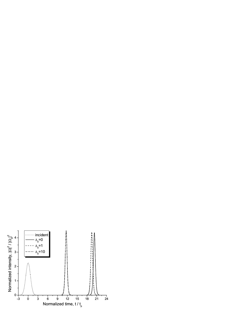
Figure 1: Intensity profiles of the $3\pi$ pulse transmitted through the two-level medium with different levels of inhomogeneous broadening. The thickness of the medium $L=100\lambda$.

First of all, let us consider the influence of inhomogeneous broadening on the dynamics of self-induced transparency (SIT) soliton formation. We take very short pulses containing only $N=25$ cycles. Such small duration is convenient from the standpoint of calculation speed, while, at the same time, it is not too short to break the rotating-wave approximation used in the Bloch equations. Anyway, the results can be rescaled for other values of $t_{p}$. As an example, let us consider the propagation characteristics of the $3\pi$ pulse (with amplitude $\Omega_{p}=1.5\Omega_{0}$). Figure 1 shows the results of transmission of such a pulse through the two-level medium of thickness $L=100\lambda$. This figure demonstrates some important aspects to be mentioned here: (i) the influence of inhomogeneous broadening appears when $\Delta_{0}\sim 1$, (ii) increasing $\Delta_{0}$ leads to the rise in pulse speed in conformity with the previous studies [26]. These facts imply that our method of calculation works well, so we can directly proceed to the topic of this paper.

The dynamics of soliton formation are traced in Fig. 2 where the change in peak intensity of the pulse as it propagates in the medium is depicted. As previously, the incident pulse has the area $3\pi$. The final, quasistationary state (the intensity of the formed soliton) is almost identical in homogeneous and inhomogeneous broadening cases, while the initial behaviour differs strongly. The pulse in homogeneously broadened medium ($\Delta_{0}=0$) experiences strong compression soon after incidence and then, through sharp oscillations of peak intensity, reaches quasistationary, solitonic form. These oscillations are analogous to those in the area dynamics studied by Yu et al. [26] and are characteristic for this case. Introduction of inhomogeneous broadening (see the curve for $\Delta_{0}=1$) makes these oscillations less pronounced, while, for $\Delta_{0}\gg 1$, they are entirely smoothed out. One can conclude that for smaller broadenings, the pulse can be stronger compressed during the transient process of soliton formation.

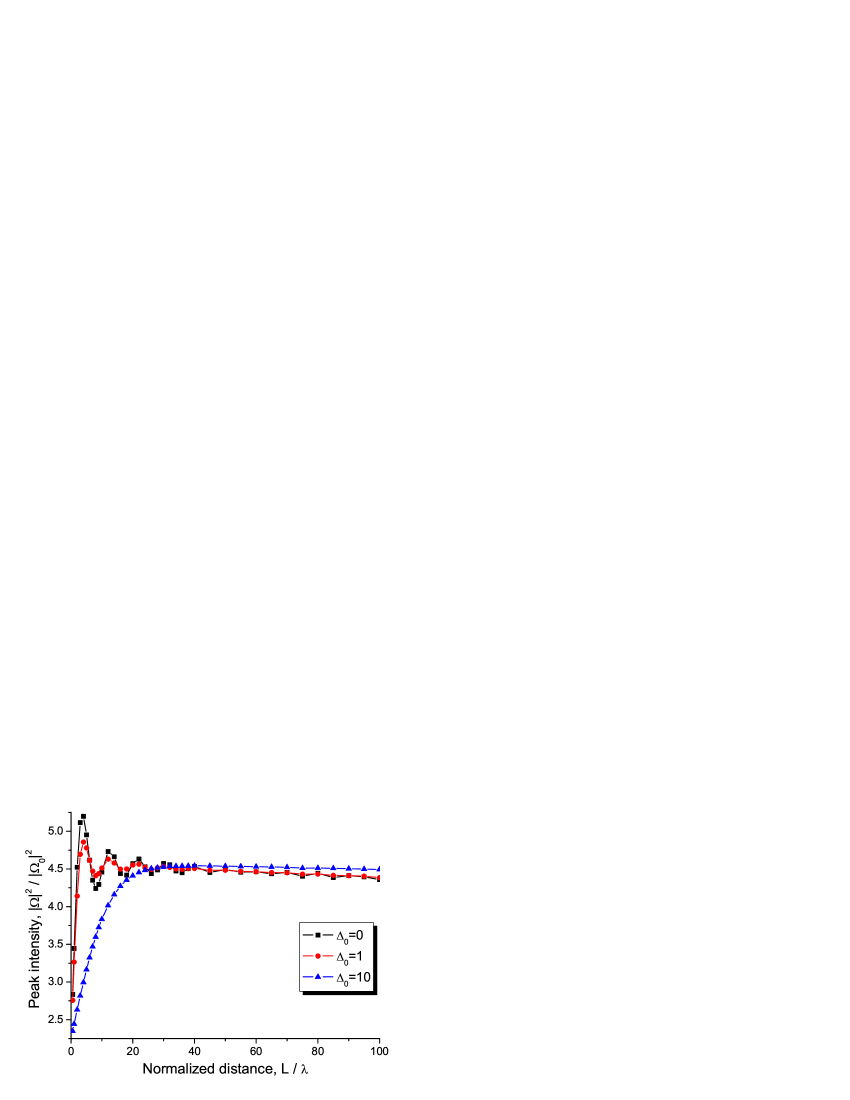
Figure 2: (Colour online) Peak intensity of the $3\pi$ pulse as a function of distance traversed through the two-level medium with different levels of inhomogeneous broadening.

As another measure of inhomogeneous broadening, we will use the mean value of population difference calculated the same way as $\rho$, namely

$$\widetilde{W}=\int W(\delta)g(\delta)d\delta.$$ (8)

In the limit of homogeneous broadening, when all the atoms have the same resonant frequency, this integrated population difference gives simply population difference $W$. Under the influence of, say, $2\pi$ pulse, $\widetilde{W}$ demonstrates typical cycle of inversion depicted in Fig. 3(a): beginning at the ground state ($\widetilde{W}=1$), the medium switches to the fully inverted state ($\widetilde{W}=-1$) and subsequently returns to the ground one ($\widetilde{W}=1$). The same behaviour is seen in Fig. 3(b) for $\Delta_{0}=0.1$ which is effectively still homogeneous case. As the inhomogeneous width of the spectral line grows, the energy of the pulse distributes over atoms with different resonant frequencies, so that the integral value $\widetilde{W}$ cannot reach the full inversion as shown in Fig. 3(c) for $\Delta_{0}=1$. For strong inhomogeneous broadening [$\Delta_{0}\gg 1$, see Fig. 3(d)], $\widetilde{W}$ stays near the ground state at every time instant. In the next section, we will discuss the implications of these population difference dynamics for collisions of solitons.

Figure 3: Dynamics of the integrated population difference $\widetilde{W}$ at the entrance of the two-level medium with different levels of inhomogeneous broadening. The incident pulse has the area $2\pi$.

4 Collisions

Figure 4: Intensity profiles of (a) the $2\pi$ forward propagating (FP) and (b) the $3\pi$ backward propagating (BP) pulses after the collision inside the two-level medium with different levels of inhomogeneous broadening. The thickness of the medium $L=100\lambda$. The profiles are recorded at right and left boundaries of the medium, respectively.

In this section, we study influence of inhomogeneous broadening on the inelastic collisions of counter-propagating pulses in two-level medium. We are especially interested in the so-called asymmetric collisions when two colliding solitons are not identical. It was shown previously [18] that in the case $\Delta_{0}=0$, such a collision can result in total destruction of one of the solitons if the initial parameters of the pulses are chosen properly. Since this effect is accompanied by strong absorption of light in the point of collision, it was called the controlled absorption of the soliton and used as a source of diode action [27]. But what if $\Delta_{0}$ is not zero?

Let us consider the collision of two pulses propagating in the two-level medium of thickness $L=100\lambda$: the first, conventionally called forward propagating (FP, from left to right), is the $2\pi$ pulse ($\Omega_{p}=\Omega_{0}$), while the second, backward propagating (BP, from right to left), is the $3\pi$ pulse ($\Omega_{p}=1.5\Omega_{0}$). The results of collisions (profiles of FP and BP transmitted radiation) for different levels of inhomogeneous broadening are shown in Fig. 4. One can see that at low broadenings ($\Delta_{0}=0.1$ and $1$), the inelastic collision results in total breakdown of the FP $2\pi$ pulse: there is no soliton at the exit of the medium. The radiation contains low-intensity oscillations, while most part of energy is trapped by the medium around the point of collision as seen in Fig. 5 where the distribution of the integrated population difference $\widetilde{W}$ after the collision is plotted. For larger values of $\Delta_{0}$, the FP soliton appears at the exit and its intensity grows with increasing $\Delta_{0}$ as is clearly seen in Fig. 4(a). Simultaneously, the excitation of medium diminishes: obviously, the strong inhomogeneous broadening cannot provide interpulse interaction large enough to effectively trap radiation. It is also should be noted that the BP $3\pi$ pulse also loses part of its energy due to collision, since the peak intensity drops from about $4.5\Omega_{0}^{2}$ (see Fig. 1 or 2) to approximately $3\Omega_{0}^{2}$ (at $\Delta_{0}=0.1$) and $2.5\Omega_{0}^{2}$ (at $\Delta_{0}=3$) and grows again for larger broadenings (see Fig. 4(b)). Nevertheless, the BP pulse is always present at the exit of the medium and can be considered as means for controlling less intensive FP soliton.

Figure 5: Distribution of the integrated population difference $\widetilde{W}$ along the two-level medium after the collisions depicted in Fig. 4. The distributions are plotted at the instant $100t_{p}$.

These relationships can be traced in more detail in Fig. 6 where one can see the dependencies of the part of the FP pulse energy transmitted through the medium and of the peak intensity of the transmitted soliton on the parameter of inhomogeneous broadening $\Delta_{0}$. It should be said that the transmitted energy is present not only in the form of soliton but also as unstructured radiation (dispersive waves). The difference can be clearly seen since the SIT solitons always have characteristic shape described by hyperbolic secant. The curves for the two variants of light-matter coupling are shown in Fig. 6. First, let us discuss the case of strong coupling ($\omega_{L}t_{p}=0.1$) corresponding to the results represented in Figs. 4 and 5. The soliton is absent at the exit at low values of broadening ($\Delta_{0}\lesssim 2.5$), though the substantial part of its energy (up to $50\%$) is transmitted in the form of low-intensity oscillations like those discussed above. The minimal value of transmitted energy (only about $6\%$) is observed at $\Delta_{0}\simeq 2.2$. Further increase in broadening leads to the rapid jump of transmitted energy corresponding to appearance of the single solitary pulse at the exit. Subsequently monotonous growth of transmitted energy and peak intensity of soliton occurs as is clearly demonstrated in Fig. 6.

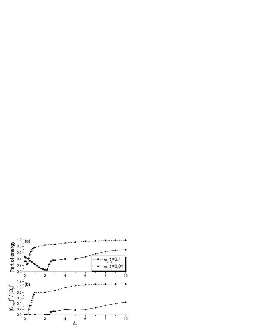
Figure 6: Dependence of (a) part of energy of $2\pi$ pulse transmitted in forward direction (by the instant $100t_{p}$) and (b) the peak intensity of transmitted soliton on the level of inhomogeneous broadening $\Delta_{0}$. The curves are shown for two strengths of light-matter coupling.

Weakening the light-matter interaction ($\omega_{L}t_{p}=0.01$) results in the pronounced shrinkage of the range of broadenings where the transmitted soliton is absent. At the same time, the minimum of transmitted energy shifts to the lower value of $\Delta_{0}$ and has significantly larger magnitude. At large broadenings, the pulses experienced the collision are more intensive than in the previous case and have the parameters close to the nonperturbed solitons. Finally, Fig. 7 demonstrates similar dependencies of the transmitted energy for the BP $3\pi$ pulse. It is seen that increase in the light-matter coupling results in reinforcement of inelasticity, since the pulse loses considerably more energy due to collision at $\omega_{L}t_{p}=0.1$ than in the case of $\omega_{L}t_{p}=0.01$. It should be also noted that the position of the minimum at $\omega_{L}t_{p}=0.1$ approximately coincides with that of Fig. 6(a); it is not so evident for $\omega_{L}t_{p}=0.01$. Nevertheless, one can say that there exists the optimal inhomogeneous broadening for observation of inelastic soliton collisions.

Figure 7: The same as in Fig. 6(a) but for $3\pi$ pulse transmitted in backward direction.

5 Conclusion

This study of coherent pulse propagation in the two-level medium is focused on the influence of inhomogeneous broadening on the SIT soliton formation and on the collisions of solitons. Though the main features of these processes remain unchanged, there are some interesting details which distinguish the case of strongly inhomogeneous broadening from its homogeneous counterpart. Formation of the SIT soliton in the homogeneously broadened medium is accompanied by the characteristic oscillations of pulse intensity (and its area), so that there is a distance of optimal compression of the pulse. At this distance, the pulse is more intensive than after ending of the formation process. In strongly inhomogeneously broadened case, these oscillations are entirely washed out and, hence, the pulse cannot be compressed more than it occurs in the final state of SIT soliton. The inelastic collisions of counter-propagating SIT solitons has the optimal conditions as well: there is a nonzero level of inhomogeneous broadening which provides the optimal trapping of radiation by the medium due to the collision. Further increasing the width of broadened line or decreasing the light-matter coupling strength (e.g. due to diluting the medium) results in sharp rising of elasticity of collisions. We believe that the results of this study will be helpful for understanding of some subtle details of light-matter interaction.

References

References

- [1] McCall S L and Hahn E L 1967 Phys. Rev. Lett. 18 908.
- [2] McCall S L and Hahn E L 1969 Phys. Rev. 183 457.
- [3] Allen L and Eberly J H 1975 Optical Resonance and Two-Level Atoms (New York: Wiley).
- [4] Kryukov P G and Letokhov V S 1970 Sov. Phys. Usp. 12 641.
- [5] Lamb Jr G L 1971 Rev. Mod. Phys. 43 99.
- [6] Poluektov I A, Popov Yu M and Roitberg V S 1975 Sov. Phys. Usp. 17 673.
- [7] Maimistov A I, Basharov A M, Elyutin S O and Sklyarov Yu M 1990 Phys. Rep. 191 1.
- [8] Bowden C M and Dowling J P 1993 Phys. Rev.A 47 1247.
- [9] Afanas’ev A A, Cherstvy A G, Vlasov R A and Volkov V M 1999 Phys. Rev.A 60 1523.
- [10] Ziolkowski R W, Arnold J M and Gogny D M 1995 Phys. Rev.A 52 3082.
- [11] Novitsky D V 2012 Phys. Rev.A 86 063835.
- [12] Bowden C M, Postan A and Inguva R 1991 J. Opt. Soc. Am.B 8 1081.
- [13] Crenshaw M E, Scalora M and Bowden C M 1992 Phys. Rev. Lett. 68 911.
- [14] Crenshaw M E 1996 Phys. Rev.A 54 3559.
- [15] Afanas’ev A A, Vlasov R A, Khasanov O K, Smirnova T V and Fedorova O M 2002 J. Opt. Soc. Am.B 19 911.
- [16] Kozlov V V 1997 Phys. Rev.A 56 1607.
- [17] Shaw M J and Shore B W 1990 J. Opt. Soc. Am.B 8 1127.
- [18] Novitsky D V 2011 Phys. Rev.A 84 013817.
- [19] Kozhekin A and Kurizki G 1995 Phys. Rev. Lett. 74 5020.
- [20] Kurizki G, Petrosyan D, Opatrny T, Blaauboer M and Malomed B 2002 J. Opt. Soc. Am.B 19 2066.
- [21] Novitsky D V 2009 Phys. Rev.A 79 023828.
- [22] Nakazawa M, Kimura Y, Kurokawa K and Suzuki K 1992 Phys. Rev.A 45 R23.
- [23] Nakazawa M, Suzuki K, Kimura Y, and Kubota H 1992 Phys. Rev.A 45 R2682.
- [24] Maimistov A I and Manykin E A 1983 Sov. Phys. JETP 58 685.
- [25] Kozlov V V and Fradkin E E 1996 JETP 82 46.
- [26] Yu X Y, Liu W and Li C 2011 Phys. Rev.A 84 033811.
- [27] Novitsky D V 2012 Phys. Rev.A 85 043813.
- [28] Taflove A 1995 Computational Electrodynamics (Boston: Artech House).
- [29] Anantha V and Taflove A 2002 IEEE Trans. Antennas Propag. 50 1337.
- [30] Fleck J A 1970 Phys. Rev.B 1 84.
- [31] Forysiak W and Moloney J V 1992 Phys. Rev.A 45 3275.
- [32] Forysiak W and Moloney J V 1992 Phys. Rev.A 45 8110.
- [33] Ablowitz M J, Kaup D J and Newell A C 1974 J. Math. Phys. 15 1852.
- [34] Kaup D J 1977 Phys. Rev.A 16 704.
- [35] Ablowitz M J and Segur H 1981 Solitons and the Inverse Scattering Transform (SIAM Studies in Applied Mathematics).
- [36] Slusher R E and Gibbs H M 1972 Phys. Rev.A 5 1634.
- [37] Novitsky D V 2010 Phys. Rev.A 82 015802.