Subsystem density functional theory with meta generalized gradient approximation exchange-correlation functionals

Abstract

We analyze the methodology and the performance of subsystem density functional theory (DFT) with meta-generalized gradient approximation (meta-GGA) exchange-correlation functionals for non-bonded systems. Meta-GGA functionals depend on the Kohn-Sham kinetic energy density (KED), which is not known as an explicit functional of the density. Therefore, they cannot be directly applied in subsystem DFT calculations. We propose a Laplacian-level approximation to the KED which overcomes the problem and provides a simple and accurate way to apply meta-GGA exchange-correlation functionals in subsystem DFT calculations. The so obtained density and energy errors, with respect to the corresponding supermolecular calculations, are comparable with conventional approaches, depending almost exclusively on the approximations in the non-additive kinetic embedding term. An embedding energy error decomposition explains the accuracy of our method.

I Introduction

Subsystem density functional theory Cortona (1991); Wesolowski and Weber (1996); Wesolowski (2006); Neugebauer (2010); Jacob and Neugebauer (2014); Krishtal et al. (2015) is nowadays attracting increasing interest in the density functional theory (DFT) Hohenberg and Kohn (1964); Kohn and Sham (1965) community. This is due to its promise of achieving potentially exact results at a reduced computational cost, as well as to the high insight into the nature of interacting systems provided by the associated embedding potentials. Thus, numerous applications related to non-covalent Wesolowski et al. (1996); Wesolowski (1997); Wesołowski et al. (1998); Wesolowski and Tran (2003); Kevorkyants et al. (2006); Dulak and Wesolowski (2007); Dułak et al. (2007); Garcia Lastra et al. (2008); Götz et al. (2009); Fradelos and Wesolowski (2011); Constantin et al. (2011a); Laricchia et al. (2011a, b); Laricchia et al. (2012); Fabiano et al. (2014a); Laricchia et al. (2013, 2014); Schluns et al. (2015); Kevorkyants et al. (2014) as well as covalent bonded systems Jacob and Visscher (2008); Fux et al. (2008); Beyhan et al. (2010); Fux et al. (2010) have been considered. In addition, the frozen density embedding (FDE) method Wesolowski (2006); Wesolowski and Warshel (1993); Hodak et al. (2008) has emerged as a practical tool for efficient simulations of different properties Neugebauer et al. (2005a); Jacob et al. (2006); Neugebauer et al. (2005b); Hodak et al. (2008); Kaminski et al. (2010); Fradelos and Wesolowski (2011); Kiewisch et al. (2013). We also recall that the FDE method with the iterative procedure of Ref. Wesolowski and Weber, 1996 is a computational implementation of the subsystem DFT.

However, the accuracy of subsystem DFT calculations is practically limited by two factors. First, the term describing the interaction energy between different subsystems depends on the non-additive kinetic energy (KE), which must be described by an explicit density functional. Second, the embedding potential, which is required to describe the mutual interaction between the subsystems, must be a local multiplicative potential. Thus, it can contain only local or semilocal approximations for the non-additive contribution of the kinetic and exchange-correlation (XC) terms to the embedding potential. Nevertheless, both limiting factors have currently been, at least partially, overcome. In fact, past years have seen the development of numerous KE functionals which can be suitable for subsystem DFT: GGA functionals Constantin et al. (2011a); Laricchia et al. (2011a); Tran et al. (2002); Lee et al. (1991); Lembarki and Chermette (1994); Thakkar (1992), Laplacian-level meta-GGA functionals Laricchia et al. (2014) and non-decomposable approach Garcia Lastra et al. (2008). For a recent review of all KE functionals see Ref. Tran and Wesolowski, 2013. Moreover, several works have extended the subsystem formulation of DFT beyond the conventional Kohn-Sham (KS) framework, considering e.g., hybrid functionals Laricchia et al. (2010), embedded interacting wave functions Wesołowski (2008), orbital-dependent effective exact exchange methods Laricchia et al. (2011b); Jacob et al. (2005), or density matrix Pernal and Wesolowski (2009). Nevertheless, to date, no attempt has been made to consider subsystem DFT calculations using meta generalized gradient approximation (meta-GGA) XC functionals.

A meta-GGA XC functional is defined by the general formula

$$E_{xc}=\int e_{xc}(\rho(\mathbf{r}),\nabla\rho(\mathbf{r}),\tau^{\text{KS}}(\mathbf{r}))d\mathbf{r}\ ,$$ (1)

where $e_{xc}$ is the XC energy density, $\rho$ is the electron density and

$$\tau^{\text{KS}}(\mathbf{r})=\frac{1}{2}\sum_{i}^{\mathrm{occ.}}\left|\nabla\phi_{i}^{\text{KS}}(\mathbf{r})\right|^{2}$$ (2)

is the positive-defined KS kinetic-energy density (KED), with $\phi_{i}^{\text{KS}}$ being the occupied KS orbitals of the system. Meta-GGAs are attracting increasing popularity Tao et al. (2003); Perdew et al. (2009); Constantin et al. (2011b); Constantin et al. (2012); Constantin et al. (2013a); Van Voorhis and Scuseria (1998); Schmider and Becke (1998); Zhao and Truhlar (2006); Peverati and Truhlar (2012); Ruzsinszky et al. (2012); Sun et al. (2012, 2013a, 2015); Wellendorff et al. (2014); Mardirossian and Head-Gordon (2015) because they can satisfy numerous exact constraints of the XC energy Tao et al. (2003); Perdew et al. (2009); Constantin et al. (2012); Constantin et al. (2013b); Della Sala et al. (2015), achieve a remarkable level of accuracy Constantin et al. (2013a); Van Voorhis and Scuseria (1998); Schmider and Becke (1998); Zhao and Truhlar (2006); Peverati and Truhlar (2012); Xiao et al. (2013); Sun et al. (2013b); Staroverov et al. (2004); Adamo et al. (2000); Riley et al. (2007); Andersen et al. (2012); Sun et al. (2015); Luo et al. (2012); Sun et al. (2011); Hao et al. (2013); Fabiano et al. (2014b), and describe excitonic effects in crystals Nazarov and Vignale (2011). In short, meta-GGA functionals has much larger accuracy/computational cost than GGAs, and thus should be preferred to the latter.

However, $\tau^{\text{KS}}$ is not an explicit functional of the density, thus the implementation of meta-GGA functionals within the conventional KS scheme is not straightforward Arbuznikov and Kaupp (2003a), since it requires the calculation of $\delta\tau^{\text{KS}}/\delta\rho$. Thus, meta-GGAs are often implemented within a Generalized Kohn-Sham scheme (GKS) Seidl et al. (1996). For this reason, so far, meta-GGA XC functionals have never been employed in subsystem DFT calculations.

In this paper we consider this issue and develop the theory and the methodology required to perform subsystem DFT calculations at the meta-GGA level. In particular, we consider proper semilocal approximations for the XC embedding contributions and test them on a set of non-covalent complexes assessing the accuracy of the resulting energies and densities.

Thus, the paper is organized as follows: in section II we present the general theory for subsystem DFT with arbitrary orbital-dependent XC functionals (thus including both meta-GGA and hybrid functionals) as well as different schemes to approximate the KED; Computational details are reported in section III; Results for non-covalent complexes are presented in section IV. Finally, in Section V we summarize our conclusions.

II Theory

II.1 Subsystem DFT with arbitrary orbital-dependent XC functionals

Within the subsystem formulation of density functional theory a given system is partitioned into two subsystems $A$ and $B$, each defined by its nuclear potential $v_{\text{nuc}}^{A}(\mathbf{r})$ and $v_{\text{nuc}}^{B}(\mathbf{r})$, respectively. Accordingly, the electron density of the total system is constructed as $\rho_{A+B}=\rho_{A}+\rho_{B}$, where the two subsystem densities integrate to $N_{A}$ and $N_{B}$, respectively. For simplicity we focus here on the case where $N_{A}$ and $N_{B}$ are integer numbers.

The ground-state solution of the problem is given by the set of coupled equations

$$\frac{\delta F_{\text{HK}}[\rho_{A}]}{\delta\rho_{A}(\mathbf{r})}+v^{A}_{\text{emb}}(\mathbf{r})+v^{A}_{\text{nuc}}(\mathbf{r}) = \mu$$ (3)

$$\frac{\delta F_{\text{HK}}[\rho_{B}]}{\delta\rho_{B}(\mathbf{r})}+v^{B}_{\text{emb}}(\mathbf{r})+v^{B}_{\text{nuc}}(\mathbf{r}) = \mu\ ,$$ (4)

where $F_{\text{HK}}$ is the universal functional of Hohenberg and Kohn, $\mu$ is the chemical potential (which is, in the case of the exact theory, equal in the two subsystems and equal to the supramolecular one Fabiano et al. (2014a); Krishtal et al. (2015); Gritsenko (2013)) and

$$v_{\text{emb}}^{I}(\mathbf{r})=\frac{\delta F_{\text{HK}}[\rho_{I}+\rho_{II}]}{\delta\rho_{I}(\mathbf{r})}-\frac{\delta F_{\text{HK}}[\rho_{I}]}{\delta\rho_{I}(\mathbf{r})}+v_{\text{ext}}^{II}(\mathbf{r})$$ (5)

is the embedding potential Laricchia et al. (2010) with $I=A,B$ and $II=B,A$, respectively (this convention will be used throughout).

In this work we consider for $F_{\text{HK}}$ the following partition:

$$F_{\text{HK}}[\rho]=F_{s}[\rho]+J[\rho]$$ (6)

with

$$F_{s}[\rho]=\min_{\Phi\rightarrow\rho}\left\{\langle\Phi|\hat{T}|\Phi\rangle+E_{xc}[\{\phi_{i}\}]\right\}$$ (7)

where $\rho$ is any $N$-representable electron density, $J$ is the classical Coulomb energy, $\hat{T}$ is the KE operator, $E_{xc}$ is a proper orbital-dependent XC functional (e.g. in the form given by Eq. (1)), $\Phi$ is a Slater determinant, and $\{\phi_{i}\}$ are its single-particle orbitals. Equation (7) is quite general and includes not only meta-GGA functionals, but all the orbital-dependent ones. Then, Eqs. (3) and (4) become

$$\frac{\delta F_{s}[\rho_{I}]}{\delta\rho_{I}(\mathbf{r})}+\frac{\delta J[\rho_{I}]}{\delta\rho_{I}(\mathbf{r})}+v^{I}_{\text{emb}}(\mathbf{r})+v^{I}_{\text{nuc}}(\mathbf{r})=\mu\;\;,$$ (8)

and the embedding potential of Eq. (5) can be written as

$$v_{\text{emb}}^{I}(\mathbf{r})=v_{\text{ext}}^{II}(\mathbf{r})+\frac{\delta J[\rho_{II}]}{\delta\rho_{II}(\mathbf{r})}+\frac{\delta F_{s}^{\text{nadd}}[\rho_{I},\rho_{II}]}{\delta\rho_{I}(\mathbf{r})}$$ (9)

where

$$F_{s}^{\text{nadd}}[\rho_{A},\rho_{B}]=F_{s}[\rho_{A}+\rho_{B}]-F_{s}[\rho_{A}]-F_{s}[\rho_{B}]$$ (10)

is the non-additive contribution to the kinetic plus XC energy and we used the fact that the Coulomb potential is additive.

At this point, following the GKS scheme Seidl et al. (1996); Laricchia et al. (2010), we introduce, for each subsystem (for example $I$) an auxiliary system of particles having the following properties: (i) it has the same ground-state density as our original embedded subsystem $I$; (ii) it is described by a single Slater determinant $\Phi^{I}$; (iii) the ground-state energy is the minimum of the energy functional

$$E[\Phi^{I}]=\langle\Phi^{I}|\hat{T}|\Phi^{I}\rangle+E_{xc}[\{\phi^{I}_{i}\}]+\int w^{I}(\mathbf{r})\rho_{I}(\mathbf{r})d^{3}\mathbf{r}\ ,$$ (11)

where $w$ is a (yet unknown) external local potential.

The ground-state energy of this system is defined via the constrained search procedure as

$$E_{0} = \min_{\rho_{I}\rightarrow N_{I}}\left\{\min_{\Phi^{I}\rightarrow\rho_{I}}E[\Phi^{I}]\right\}$$ (12)

$$= \min_{\rho_{I}\rightarrow N_{I}}\left\{F_{s}[\rho_{I}]+\int w^{I}(\mathbf{r})\rho_{I}(\mathbf{r})d^{3}\mathbf{r}\right\}\,.$$

Hence, the ground-state is described by the Euler equation

$$\frac{\delta F_{s}[\rho_{I}]}{\delta\rho_{I}(\mathbf{r})}+w^{I}(\mathbf{r})=\mu\ .$$ (13)

Comparing Eqs. (8) and (13) and making use of the property (i) we thus find

$$w^{I}(\mathbf{r})=v^{I}_{\text{nuc}}(\mathbf{r})+\frac{\delta J[\rho_{I}]}{\delta\rho_{I}(\mathbf{r})}+v^{I}_{\text{emb}}(\mathbf{r})\,.$$ (14)

On the other hand, properties (ii) and (iii) imply directly that the ground-state of the auxiliary system is described by the set of single-particle equations

$$\left[-\frac{1}{2}\nabla^{2}+w^{I}(\mathbf{r})\right]\phi_{i}^{I}(\mathbf{r})+\frac{1}{2}\frac{\delta E_{xc}[\{\phi^{I}_{i}\}]}{\delta\phi^{I}_{i}(\mathbf{r})}=\epsilon^{I}_{i}\phi^{I}_{i}(\mathbf{r})\ ,$$ (15)

where we assumed real orbitals and $\epsilon^{I}_{i}$ are Lagrange multipliers to ensure orbital orthonormality. For a meta-GGA functional the last term on the left hand side can be evaluated as Arbuznikov and Kaupp (2003b); Arbuznikov et al. (2002)

$$\frac{\delta E_{xc}}{\delta\phi_{i}}=2\left[\frac{\partial e_{xc}}{\partial\rho}\phi_{i}+\left(\nabla\cdot\frac{\partial e_{xc}}{\partial\nabla\rho}\right)\phi_{i}-\frac{1}{2}\nabla\cdot\left(\frac{\partial e_{xc}}{\partial\tau}\nabla\phi_{i}\right)\right]\ .$$ (16)

Combining Eq. (14) with Eq. (15) the operational equations to solve the subsystem ground-state problem are, finally:

$$\left[-\frac{1}{2}\nabla^{2}+\frac{\delta J[\rho_{A}]}{\delta\rho_{A}(\mathbf{r})}+v^{A}_{\text{emb}}(\mathbf{r})+v^{A}_{\text{nuc}}(\mathbf{r})\right]\phi^{A}_{i}(\mathbf{r})+$$

$$\quad\quad\quad\quad+\frac{1}{2}\frac{\delta E_{xc}[\{\phi^{A}_{i}\}]}{\delta\phi^{A}_{i}(\mathbf{r})}=\epsilon^{A}_{i}\phi^{A}_{i}(\mathbf{r})$$ (17)

$$\left[-\frac{1}{2}\nabla^{2}+\frac{\delta J[\rho_{B}]}{\delta\rho_{B}(\mathbf{r})}+v^{B}_{\text{emb}}(\mathbf{r})+v^{B}_{\text{nuc}}(\mathbf{r})\right]\phi^{B}_{i}(\mathbf{r})+$$

$$\quad\quad\quad\quad+\frac{1}{2}\frac{\delta E_{xc}[\{\phi^{B}_{i}\}]}{\delta\phi^{B}_{i}(\mathbf{r})}=\epsilon^{B}_{i}\phi^{B}_{i}(\mathbf{r})$$ (18)

with the embedding potential $v^{I}_{\text{emb}}$ given by Eq. (9). Note that, if the embedding potential is treated exactly, Eqs. (17) and (18) admit in general multiple solutions Humbert-Droz et al. (2013); Krishtal et al. (2015); Nafziger and Wasserman (2014). Once the orbitals have been obtained, the total electron density is computed as

$$\rho_{A+B}(\mathbf{r})=\sum_{i=1}^{N_{A}}\left|\phi_{i}^{A}(\mathbf{r})\right|^{2}+\sum_{i=1}^{N_{B}}\left|\phi_{i}^{B}(\mathbf{r})\right|^{2}\ ,$$ (19)

whereas the total electronic energy is calculated as

$$E_{A+B}[\rho_{A},\rho_{B}]=\langle\Phi^{A}|\hat{T}_{s}|\Phi^{A}\rangle+\langle\Phi^{B}|\hat{T}_{s}|\Phi^{B}\rangle$$

$$+E_{xc}[\{\phi_{i}^{A}\}]+E_{xc}[\{\phi_{i}^{B}\}]+J[\rho_{A}+\rho_{B}]+$$

$$+\int\left(\rho_{A}(\mathbf{r})+\rho_{B}(\mathbf{r})\right)\left(v_{\text{nuc}}^{A}(\mathbf{r})+v_{\text{nuc}}^{B}(\mathbf{r})\right)d^{3}\mathbf{r}+F_{s}^{\text{nadd}}[\rho_{A},\rho_{B}]\ .$$

Note that the formalism introduced above is quite general and can be applied to GGA, hybrid-GGA, and meta-GGA functionals.

II.2 Non-additive embedding contributions

To perform embedding calculations according to the theory detailed in Sec. II.1 we need to compute the non-additive contribution $F_{s}^{\text{nadd}}[\rho_{A},\rho_{B}]$ (see Eq. (II.1)) and its derivatives with respect to $\rho_{A}$ and $\rho_{B}$ (see Eq. (9)). This is not an easy task for two main reasons Laricchia et al. (2010):

(i) The computation of $F_{s}[\rho_{A}+\rho_{B}]$ requires the knowledge of the ground-state Slater determinant of the total system, $\Phi^{A+B}$, which is not available by definition in a subsystem calculation. It can only be obtained by an inverse KS Zhao et al. (1995); Wu and Yang (2003); de Silva and Wesolowski (2012) calculation starting from the ground-state total density $\rho_{A+B}$ (for some examples within FDE see Refs. Roncero et al., 2008, 2009; Fux et al., 2010; Goodpaster et al., 2010, 2011).

(ii) The $F_{s}$ functional depends explicitly on the orbitals and has only an implicit dependence on the density. Therefore, to make the required functional derivatives special techniques are required, such as the optimized effective potential method Kümmel and Kronik (2008); Jacob (2011); Heßelmann et al. (2007); Staroverov et al. (2006); Heaton-Burgess et al. (2007).

Consequently, in search of a practical computational procedure to perform subsystem DFT calculations with meta-GGA XC functionals, we propose to consider, in analogy with Refs. Laricchia et al., 2010; Laricchia et al., 2011b, in Eq. (10) the semilocal approximation

$$F_{s}[\rho] \approx \widetilde{F}_{s}[\rho]=\widetilde{T}_{s}[\rho]+\widetilde{E}_{xc}[\rho]\ ,$$ (20)

$$F_{s}^{nadd}[\rho] \approx \widetilde{F}_{s}^{nadd}[\rho]=\widetilde{T}_{s}^{nadd}[\rho]+\widetilde{E}_{xc}^{nadd}[\rho]\ ,$$ (21)

where the tilde denotes that an approximated (semilocal) functional of the density is used.

For the kinetic term standard semilocal approximations can be employed Constantin et al. (2011a); Laricchia et al. (2011a); Tran et al. (2002); Lembarki and Chermette (1994); Thakkar (1992); Tran and Wesolowski (2013). For the XC part, instead, two main possibilities can be envisaged:

• As a first simple option it is possible to use for $\widetilde{E}_{xc}$ the GGA functional “most similar” to the meta-GGA functional used for subsystems calculations. For example, if the TPSS Tao et al. (2003) functional is used for subsystems calculations, the natural choice will be to use the PBE functional for the non-additive contribution. In fact, the TPSS functional has been constructed as an extension of the PBE functional. This choice resembles that of Refs. Laricchia et al., 2010; Laricchia et al., 2011b and may be expected to yield reasonable results. The accuracy of this combination will be verified in section IV.

• A second, possibly better, choice is to retain for $\widetilde{E}_{xc}$ the meta-GGA form, but replacing $\tau$ with a suitable semilocal approximation. We recall that this is in general a very hard task Yang et al. (1986); García-Aldea and Alvarellos (2007). However, for our purposes we only need the non-additive XC energy and, as shown in section IV, a large error cancellation effect can thus be expected.

II.3 Semilocal models for the kinetic energy density

In this subsection we consider the construction of semilocal models for the KED. However, since the KED is not an observable, it is defined only up to a gauge integrating to zero (and vanishing in the functional derivative). Thus, to fix our working definition of the KED we decide to consider here only the positive-defined KED (Eq. (2); see Ref. Ayers et al., 2002 for a discussion on this topic), which is also the most commonly used in meta-GGA XC functionals.

To model the positive-defined KED in our subsystem DFT calculations we consider the following two semilocal approximations:

$$\tilde{\tau} \approx \tau^{\text{TF}}+\tau^{W}\doteq\tau^{1}$$ (22)

$$\tilde{\tau} \approx \tau^{\text{revAPBEK}}+\frac{20}{9}\tau^{\text{TF}}q\doteq\tau^{L},$$ (23)

where $\tau^{\text{TF}}=(3/10)(3\pi^{2})^{2/3}\rho^{5/3}$ is the Thomas-Fermi (TF) kinetic energy density Thomas (1926); Fermi (1928, 1927), $\tau^{W}=(5/3)\tau^{\text{TF}}s^{2}=|\nabla\rho|^{2}/(8\rho)$ is the von Weizsäcker kinetic energy density von Weizsäcker (1935) (with $s=|\nabla\rho|/[2(3\pi^{2})^{1/3}\rho^{4/3}]$ the reduced gradient), $\tau^{\text{revAPBEK}}$ is the revAPBEK kinetic energy density Constantin et al. (2011a); Laricchia et al. (2011a), and $q=\nabla^{2}\rho/[4(3\pi^{2})^{2/3}\rho^{5/3}]$ is the reduced Laplacian.

The $\tau^{1}$ model of Eq. (22) is a simple GGA model that is exact for a uniform density perturbed by a small-amplitude short-wavelength density wave and motivated by the basic requirements that $\tau\approx\tau^{\text{TF}}$ in the slowly-varying density limit and $\tau\approx\tau^{W}$ Della Sala et al. (2015) in tail regions (where $\tau^{\text{TF}}\rightarrow 0$) and iso-orbital regions. Moreover, this simple model fulfills the important constraint $\tau^{W}\leq\tau$, i.e. that $0\leq z\leq 1$, with $z=\tau^{W}/\tau$, which has actually been used in the construction of several meta-GGA XC functionals Tao et al. (2003).

The $\tau^{L}$ model of Eq. (23) is a Laplacian-level meta-GGA model and requires several considerations:

• We first recall that $(20/9)\tau^{\text{TF}}q=(1/6)\nabla^{2}\rho$. Thus, the kinetic energy and potential corresponding to $\tau^{L}$ are identical with the revAPBEK ones (recall that a term proportional to the Laplacian of the density does not contribute to the energy and the potential). If the revAPBEK functional is used for $\tilde{T}_{s}$ and $\tilde{T}_{s}^{nadd}$ in Eqs. (20) and (21), then the revAPBEK KE approximation is “de facto” the only functional approximation used in the subsystem DFT meta-GGA calculation. In fact, in our implementation we use the same KE functional in both $\tau^{L}$ and $\widetilde{T}_{s}^{nadd}[\rho]$.

• The term containing $q$ is of fundamental importance to reproduce the correct KE density Yang et al. (1986); García-Aldea and Alvarellos (2007)). In Eq. (23) the coefficient of the reduced Laplacian term comes from the lowest-order Laplacian contribution to the second-order gradient expansion of the KE Brack et al. (1976); Kirzhnits (1957). Other coefficients could be used as well Yang et al. (1986); García-Aldea and Alvarellos (2007), but we found that the non-empirical one in Eq. (23) is quite accurate for our purpose, even if Eq. (23) is not exact in the asymptotic region (see Appendix A).

• The revAPBEK functional, which is used in the definition of $\tau^{L}$, recovers by construction the modified second-order gradient expansion of the KELee et al. (2009), which was constructed from semiclassical theory of atoms. Actually, the revAPBEK functional, which does not contain any empirical parameter fitted on kinetic energies, has been found to be very accurate for the description of non-covalent complexes within subsystem DFT Laricchia et al. (2011a). However, the accuracy of the $\tau^{L}$ model is not mandatorily related to the use of revAPBEK: other state-of-the-art GGA Constantin et al. (2011a); Laricchia et al. (2011a); Tran et al. (2002); Lee et al. (1991); Lembarki and Chermette (1994); Thakkar (1992) and meta-GGA Laricchia et al. (2014) KE approximations can be expected to yield similar accuracy.

• The Laplacian term will diverge at the core ($q\rightarrow-\infty$). However, such a bad behavior in the core region is not a problem for subsystem DFT calculations, since for the non-additive XC energy and potential these contributions cancel almost completely. This cancellation is shown in Figure 6 of Ref. Laricchia et al., 2014 where a reduced gradient and Laplacian decomposition of the non-additive KE is reported, showing that only small values of $q$ contribute significantly.

To show the physical significance of the two models introduced above and offer a preliminary test of the expectable performance, we consider their application to the test case of the Ne dimer, an example for weakly interacting systems. As meta-GGA exchange correlation functional we consider the TPSS Tao et al. (2003) one. This is in fact one of the first and most popular non-empirical meta-GGAs and is used here as an exemplary case.

In Fig. 1a we report the quantity $z=\tau^{W}/\tau$ for the two KE density approximations Eqs. (22) and (23) as a function of the distance $d$ along the dimer axis.

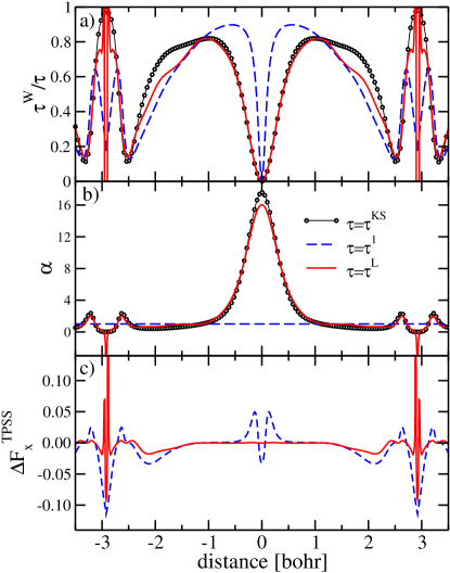
Figure 1: Plot of $z=\tau^{\text{W}}/\tau$ (panel a), $\alpha=(\tau-\tau^{W})/\tau^{\text{TF}}$ (panel b) and $\Delta F_{x}^{\text{TPSS}}$ (panel c) for the Ne dimer along the main axis computed using the kinetic energy density models of Eqs. (22) and (23).

In the middle of the bond ($d=0$) all curves go to zero, because the gradient of the density and thus $\tau^{\text{W}}$ vanish. The $\tau^{1}$ model is accurate only at few points: $|d|\approx 1$ bohr and near the core. However, exactly at the nucleus position the exact $\tau^{W}/\tau$ is close to 1 Della Sala et al. (2015); on the other hand at this point the density is very large so that $\tau^{\text{TF}}\gg\tau^{\text{W}}$, thus $\tau^{W}/\tau^{1}$ is much less than 1. The Laplacian model $\tau^{L}$ is everywhere (but in the core) much more accurate than $\tau^{1}$. In particular, it reproduces almost exactly $\tau^{\text{KS}}$ in the region $|d|\leq 1.5$ bohr.

Alternatively, in Fig. 1b we report the quantity

$$\alpha=\frac{\tau-\tau^{W}}{\tau^{\text{TF}}}=\frac{5}{3}s^{2}\left(\frac{1}{z}-1\right)$$ (24)

which is the main, direct ingredient of the meta-GGA (TPSS) exchange enhancement factor and thus on the calculation of the exchange energy. Differences about the various approaches are now more evident. For the $\tau^{1}$ model $\alpha=1$ everywhere in the space (by construction): this can be a good approximation only for slowly varying densities. Instead, for molecular systems, the exact alpha shows significant oscillations and it is very high ($\alpha\approx 17.6$) in the bond. These oscillations are correctly reproduced by the $\tau^{L}$ model, which yields a very accurate value at the bond ($\alpha\approx 16.0$). $\tau^{L}$ is significantly different from the exact one only near the core, where it is actually negative. Finally, In Fig. 1c we report the quantity

$$\Delta F_{x}^{\text{TPSS}}=F_{x}^{\text{TPSS}}(\rho,\nabla\rho,\tilde{\tau})-F_{x}^{\text{TPSS}}(\rho,\nabla\rho,\tau^{KS})$$ (25)

where $F_{x}^{TPSS}$ is the TPSS exchange enhancement factor Tao et al. (2003), so that

$$E_{x}^{\text{TPSS}}=\int\rho\epsilon_{x}^{\text{LDA}}(\rho)F_{x}^{\text{TPSS}}(\rho,\nabla\rho,\tau^{KS})d\mathbf{r}\ ,$$ (26)

where $\epsilon_{x}^{\text{LDA}}$ is the LDA exchange energy per particle. The quantity $\Delta F_{x}^{\text{TPSS}}$ indicates how much the approximation in $\tilde{\tau}$ will impact on the accuracy of the exchange energy.

The plots in Fig. 1b confirm the high accuracy of the $\tau^{L}$ model, whereas the $\tau^{1}$ model shows quite larger differences in the region $|d|<0.5$ au.

In section IV we will consider the performance of the two models for subsystem DFT calculations.

III Computational details

To assess the possibility of performing subsystem DFT calculations using meta-GGA functionals we carried on test simulations on different non-covalent complexes. To this end, for simplicity, we considered as meta-GGA XC functional the TPSS one Tao et al. (2003). Other meta-GGA XC functionals will be considered in detail in a future publication.

In our calculations we used different approximations for the non-additive XC terms. We refer to each of these using the notation method1/method2, that denotes that method1 was used for the subsystems and method2 to compute the non-additive XC contribution. In more details:

1. As a simple choice we computed the non-additive XC contributions using the PBE XC functional Perdew et al. (1996a), i.e. we set $\widetilde{E}_{xc}=E_{xc}^{PBE}$. This approach is labeled TPSS/PBE.

2. Alternatively, we computed the non-additive XC terms using the XC TPSS functional but using the $\tau^{1}$ model of Eq. (22) to mimic the positive-defined KED. This approach is named TPSS/TPSS-1.

3. Finally, we considered the same case as above but using the $\tau^{L}$ model of Eq. (23). This approach is labeled TPSS/TPSS-L. Note that in this case, because of the negative divergence of $q$, the model we use for $\tau$ is not guaranteed to respect the bound $\tau^{W}\leq\tau$. Nevertheless, the TPSS functional is numerically well defined also for $z<0$ or $z>1$; moreover these values occur only near the core which is not relevant for non-additive contributions, see point iv) of section II.3.

We remark that the first two approximations are GGA ones, while the last one is a Laplacian-level meta-GGA method. For comparison also subsystem DFT calculations using the PBE Perdew et al. (1996a) and PBE0 Adamo and Barone (1999); Perdew et al. (1996b) XC functionals were considered. The former one requires no approximations for the non-additive XC terms and implements the PBE/PBE approach; the latter one instead uses a semilocal approximation as described in Ref. Laricchia et al., 2010 and yields the PBE0/PBE approach.

In all calculations the non-additive kinetic contributions were computed using the revAPBEK kinetic functional Constantin et al. (2011a); Laricchia et al. (2011a) and a supermolecular def2-TZVPPD basis set Weigend and Ahlrichs (2005); Rappoport and Furche (2010) was employed. As the aim of this work is not to verify the absolute accuracy of the embedding approach (which depends critically on the KE approximation), but if the additional errors due to the non-additive XC approximation can be reduced or not, we believe that checking one (accurate) KE functional is enough.

All calculations have been performed using the FDE script Laricchia et al. (2010) of the TURBOMOLE program package tur . The calculation of the matrix elements of the non-additive TPSS-L XC functional (which is a Laplacian-level meta-GGA functional), has been performed as described in the Appendix A of Ref. Laricchia et al. (2014).

The complexes considered for the tests have been divided into four groups according to the character dominating their interaction:

• WI (weak interaction): He-Ne, He-Ar, Ne-Ne, Ne-Ar, CH₄-Ne, C₆H₆-Ne, CH₄-CH₄;

• DI (dipole-dipole interaction): H₂S-H₂S, HCl-HCl, H₂S-HCl, CH₃Cl-HCl, CH₃SH-HCN, CH₃SH-HCl;

• HB (hydrogen bond): NH₃-NH₃, HF-HF, H₂O-H₂O, HF-HCN, (HCONH₂)₂, (HCOOH)₂;

• CT (charge transfer): NF₃-HCN,C₂H₄-F₂,NF₃-HCN, C₂H₄-Cl₂, NH₃-F₂, NH₃-ClF, NF₃-HF, C₂H₂-ClF, HCN-ClF, NH₃-Cl₂, H₂O-ClF, NH₃-ClF.

The reference geometries and binding energies were taken from Refs. Zhao and Truhlar, 2005a, b; Wesolowski et al., 1996; Laricchia et al., 2013.

The error on the total embedding energy was computed as the difference between the energy obtained from a subsystem DFT calculation (i.e. Eq. (II.1)) and the energy ($E^{\text{GKS}}$) obtained from the corresponding supermolecular conventional calculation Laricchia et al. (2010); Laricchia et al. (2011a); Laricchia et al. (2012), i.e.

$$\Delta E=E_{A+B}[\tilde{\rho}_{A},\tilde{\rho}_{B}]-E^{\text{GKS}}[\rho_{\text{GKS}}]$$ (27)

where $\tilde{\rho}_{A}$ and $\tilde{\rho}_{B}$ are approximated embedded subsystems densities, due to the approximations in Eq. (21).

The performance of the different approaches was evaluated, within each group of complexes, by computing the mean absolute error (MAE) and the mean absolute relative error (MARE) with respect to reference binding energies Laricchia et al. (2012). Instead, to assess the performance of the methods for all the different classes of systems, we considered the quantities Laricchia et al. (2011a)

rwMAE $$= \frac{1}{4}\sum_{i=\text{WI,DI,HB,CT}}\left(\frac{MAE_{i}}{\langle MAE_{i}\rangle}\right)$$ (28)

rwMARE $$= \frac{1}{4}\sum_{i=\text{WI,DI,HB,CT}}\left(\frac{MARE_{i}}{\langle MARE_{i}\rangle}\right)$$ (29)

where $\langle MAE_{i}\rangle$ ($\langle MARE_{i}\rangle$) is the average MAE (MARE) among the different methods considered for the class of systems $i$. In this way, all the different classes of systems will have the same influence of the rwMAE (rwMARE) and methods with rwMAE (rwMARE) smaller than 1 will have better performance than the average.

The errors on the embedding densities were studied by considering the deformation density

$$\Delta\rho(\mathbf{r})=\tilde{\rho}_{A}(\mathbf{r})+\tilde{\rho}_{B}(\mathbf{r})-\rho^{\text{GKS}}(\mathbf{r})\ ,$$ (30)

where $\rho^{\text{GKS}}$ denotes the density obtained from a conventional GKS calculation. A quantitative measurement of the absolute error associated with a given embedding density was then obtained by computing the embedding density error

$$\xi=\frac{1000}{N}\int\left|\Delta\rho(\mathbf{r})\right|\,d\mathbf{r},$$ (31)

with $N$ the number of electrons. In the evaluation of $\xi$ only valence electron densities were considered. Core densities are in fact much higher than valence ones and would largely dominate. On the other hand, core densities are not very important for the determination of chemical and physical properties of the interaction between the subsystems, which are of interest here. The performance of the different approaches was evaluated by computing the MAE and the rwMAE.

IV Results

Table 1: Errors on the embedding densities for different methods as obtained using Eq. (31). At the bottom of each group of results the mean absolute error (MAE) is reported. The last row report the global rwMAE (see text for details). The best result of each line is highlighted in bold style. A star indicates the best result among meta-GGA methods.

Complex	PBE/PBE	PBE0/PBE	TPSS/PBE	TPSS/TPSS-1	TPSS/TPSS-L
weak interaction (WI)
He-Ne	0.05	0.02	0.05*	0.05*	0.05*
He-Ar	0.06	0.06	0.12	0.08	0.05*
Ne-Ne	0.04	0.02	0.06	0.04	0.03*
Ne-Ar	0.06	0.04	0.13	0.08	0.05*
CH4-Ne	0.07	0.05	0.16	0.13	0.06*
C6H6-Ne	0.13	0.11	0.25	0.27	0.13*
CH4-CH4	0.60	0.50	0.84	0.79	0.53*
MAE	0.14	0.11	0.23	0.21	0.13*
dipole-dipole interaction (DI)
H2S-H2S	1.85	1.62	1.89	1.81	1.70*
HCl-HCl	1.87	1.49	1.88	1.91	1.75
H2S-HCl	3.70	2.97	3.59	3.74	3.56
CH3Cl-HCl	2.38	1.91	2.36	2.40	2.24
CH3SH-HCN	1.72	1.61	1.74	1.64	1.58
CH3SH-HCl	4.08	3.32	3.90	4.12	3.95
MAE	2.60	2.15	2.56	2.60	2.46*
hydrogen bond (HB)
NH3-NH3	1.79	1.67	1.87	1.85	1.74
HF-HF	1.53	1.19	1.56	1.62	1.50*
H2O-H2O	2.01	1.72	2.05	2.11	1.98*
NH3-H2O	3.11	2.69	3.06*	3.19	3.08
HF-HCN	2.77	2.38	2.62*	2.84	2.75
(HCONH2)2	2.72	2.49	2.71*	2.76	2.65
(HCOOH)2	3.35	2.94	3.23*	3.45	3.37
MAE	2.47	2.15	2.44*	2.55	2.54
charge transfer (CT)
NF3-HCN	0.29	0.24	0.40	0.43	0.26*
C2H4-F2	6.35	2.75	5.68*	5.79	5.79
NF3-HNC	0.58	0.49	0.58	0.63	0.55*
C2H4-Cl2	5.77	4.32	5.85*	6.08	6.28
NH3-F2	9.60	4.38	8.48	8.60	8.58*
NF3-ClF	1.73	0.99	1.59	1.54*	1.68
NF3-HF	0.95	0.75	0.91	0.88*	0.91
C2H2-ClF	6.02	4.32	5.97*	6.77	6.51
HCN-ClF	3.21	2.33	3.08*	3.40	3.30
NH3-Cl2	7.60	5.48	7.42*	8.25	8.06
H2O-ClF	5.06	3.42	4.98	5.54	5.39*
NH3-ClF	11.19	9.37	11.00*	12.37	12.06
MAE	4.86	3.24	4.66*	5.02	4.95
rwMAE	1.00	0.79	1.12	1.14	0.97*

The errors $\xi$ on the embedding densities for the different methods are reported in Table 1. The best performance is observed for the PBE0/PBE method, which gives the smallest error for all the systems investigated. As explained in Refs. Laricchia et al., 2010, 2013; Laricchia et al., 2011b this fact traces back to the reduced self-interaction error of the PBE0 functional, which reduces the overlap between the subsystem densities. All other methods yield very close results with a rwMAE in the range $0.97-1.14$. Actually the TPSS/TPSS-L has the lowest rwMAE between these ones, showing that meta-GGA subsystem calculations can perform even better than conventional GGA calculations, despite the former include an additional approximation. Among meta-GGA methods, the TPSS/TPSS-L approach is the best for WI systems (MAE=0.13) and for DI (MAE=2.46), whereas TPSS/PBE is the best for HB and CT.

The integrated measure $\xi$ however provides only an absolute measure of the error on embedding densities, but cannot tell anything on how the error on the density is distributed in the space and what are the roles of the kinetic and XC approximations to determine such an error. Here, we aim at understanding better the importance of different approximations used in the non-additive XC term of the embedding potential.

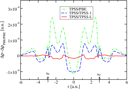
Figure 2: Plot of $\Delta\rho^{method}(z)-\Delta\rho_{PBE/PBE}(z)$ (for the Ne dimer along the main axis) computed using the kinetic energy density models of Eqs. (22) and (23) as well as the PBE XC functional for the non-additive XC embedding potential.

Thus, we consider in Fig. 2 the plot along the bond axis of the Ne-Ne complex (taken as an example) of the plane-averaged XC deformation density $\Delta\rho^{method}(z)-\Delta\rho^{PBE/PBE}(z)$, where the plane-averaged deformation density is

$$\Delta\rho(z)=\int|\Delta\rho(\mathbf{r})|dxdy\ .$$ (32)

This quantity provides in fact a measure, point by point, of the embedding density error due to the XC approximation: the PBE/PBE is in fact taken as reference because it includes only approximation due to KE. We see that, in agreement with the results of Fig. 1, the TPSS-L approximation performs very well, introducing only very small errors in the calculation of the embedding density. A larger effect is instead obtained for TPSS-1, while the use of the PBE XC functional to compute the embedding potential yields considerably larger differences.

Table 2: Embedding energy errors (mHa) for different methods and complexes. Accurate reference binding energies ($E_{b}$) from Refs. Zhao and Truhlar, 2005a, b; Wesolowski et al., 1996 are also reported in the second column. At the bottom of each group of results the mean absolute error (MAE) and the mean absolute relative error (MARE) are reported. The best result of each line is highlighted in bold style. A star indicates the best result among the ones with the TPSS functional.

Complex	$E_{b}$	PBE/PBE	PBE0/PBE	TPSS/PBE	TPSS/TPSS-1	TPSS/TPSS-L
weak interaction (WI)
He-Ne	0.06	0.08	0.03	0.03*	0.06	0.08
He-Ar	0.10	0.05	0.00	-0.01*	0.04	0.06
Ne-Ne	0.13	0.14	0.06	0.02*	0.10	0.13
Ne-Ar	0.21	0.11	0.04	-0.04*	0.06	0.11
CH4-Ne	0.35	0.12	0.04	-0.04*	0.06	0.12
C6H6-Ne	0.75	-0.03	-0.10	-0.51	-0.25	-0.01*
CH4-CH4	0.81	-0.38	-0.41	-0.82	-0.54	-0.27*
MAE		0.13	0.10	0.21	0.16	0.11*
MARE		61%	27%	39%*	52%	59%
dipole-dipole (DI)
H2S-H2S	2.63	-0.47	-0.84	-1.16	-1.07	-0.49*
HCl-HCl	3.20	0.07	-0.37	-0.70	-0.62	-0.02*
H2S-HCl	5.34	0.40	-0.42	-0.54	-0.71	0.29*
CH3Cl-HCl	5.66	0.02	-0.59	-1.14	-1.27	-0.05*
CH3SH-HCN	5.72	-1.18	-1.57	-2.09	-2.04	-1.02*
CH3SH-HCl	6.63	0.73	-0.34	-0.64	-1.06	0.54*
MAE		0.48	0.69	1.05	1.13	0.40*
MARE		10%	16%	24%	25%	9%*
hydrogen bond (HB)
NH3-NH3	5.02	-0.95	-1.32	-1.69	-1.63	-0.80*
HF-HF	7.28	0.79	0.19	-0.13	-0.03*	0.78
H2O-H2O	7.92	-0.20	-0.79	-1.11	-1.15	-0.15*
NH3-H2O	10.21	-0.44	-1.28	-1.47	-1.75	-0.36*
HF-HCN	11.33	0.43	-0.56	-0.72	-1.06	0.49*
(HCONH2)2	23.81	-4.21	-5.30	-5.95	-6.87	-3.42*
(HCOOH)2	25.74	-1.88	-3.69	-3.94	-5.61	-1.37*
MAE		1.27	1.88	2.14	2.59	1.05*
MARE		9%	13%	16%	18%	8%*
charge transfer (CT)
NF3-HCN	1.67	-0.41	-0.43	-0.95	-0.88	-0.31*
C2H4-F2	1.69	4.27	1.92	3.13*	3.42	3.87
NF3-HNC	2.31	-0.13	-0.51	-0.78	-1.11	-0.02*
C2H4-Cl2	2.60	1.52	-0.42	0.30*	-1.87	1.70
NH3-F2	2.88	6.90	2.98	5.17*	5.47	6.07
NF3-ClF	2.92	2.14	0.82	0.88	0.15*	1.95
NF3-HF	2.92	0.91	0.22	0.05*	-0.57	0.86
C2H2-ClF	6.07	3.71	1.52	2.40	1.64*	3.77
HCN-ClF	7.74	1.62	0.03	0.28	-0.27*	1.51
NH3-Cl2	7.78	2.84	0.21	1.64	0.85*	2.94
H2O-ClF	8.54	2.42	0.45	1.17	0.55*	2.45
NH3-ClF	16.92	4.44	1.31	2.35	-0.33*	5.75
MAE		2.61	0.90	1.59	1.43*	2.60
MARE		72%	30%	49%*	53%	67%
rwMAE		0.93	0.79	1.24	1.21	0.84*
rwMARE		0.98%	0.78%	1.10%	1.24%	0.91%*

We now turn to discuss the embedding energy errors, which are reported in Tab. 2. In this case the hybrid PBE0/PBE is not the best for all systems, as it was in Tab. 1. In fact, for dipole-dipole and hydrogen bond complexes the TPSS/TPSS-L method is the most accurate, closely followed by the PBE/PBE approach, whereas the PBE0/PBE is not so accurate for these systems Laricchia et al. (2012); Laricchia et al. (2011b). On the other hand, PBE0/PBE is very accurate for weakly-interacting and charge-transfer systems Laricchia et al. (2013).

A more detailed discussion of the trends is provided in subsection IV.1 where we perform an energy decomposition analysis of the embedding energy errors. Here we just note that, concerning the meta-GGA approaches, our simple Laplacian-level meta-GGA approximation (TPSS/TPSS-L) is significantly more accurate than the GGA TPSS/TPSS-1 and TPSS/PBE ones and can also slightly outperform the use of a simple GGA XC functional, such as PBE. In fact, for TPSS/TPSS-L, PBE/PBE, TPSS/PBE, and TPSS/TPSS-1 we find overall rwMAEs of 0.84, 0.93 and 1.21, 1.24, respectively.

IV.1 Error decomposition analysis

The embedding energy error for meta-GGA as well as for hybrid functionals depends on two distinct approximations, the KE and the XC energy. As discussed in Ref. Laricchia et al., 2012 this causes a subtle error cancellation effect. To understand better the error compensation issue in meta-GGA subsystem DFT calculations and analyze in detail the sources of different errors, we perform in the following an error decomposition analysis.

Following Ref. Laricchia et al., 2012 we thus write the error on the embedding energy as

$$\Delta E=\Delta T_{s}+\Delta D+\Delta E_{xc}\ ,$$ (33)

with

$$\Delta T_{s} = \widetilde{T}_{s}^{nadd}[\tilde{\rho}_{A},\tilde{\rho}_{B}]-$$

$$-\left(T_{s}[\{\phi^{\text{GKS}}_{A+B}\}]-T_{s}[\{\tilde{\phi}^{A}\}]-T_{s}[\{\tilde{\phi}^{B}\}]\right)$$

$$\Delta D = E_{ext}[\tilde{\rho}_{A+B}]+J[\tilde{\rho}_{A+B}]+\tilde{E}_{xc}[\tilde{\rho}_{A+B}]-$$

$$-\left(E_{ext}[\rho^{\text{GKS}}]+J[\rho^{\text{GKS}}]+\widetilde{E}_{xc}[\rho^{\text{GKS}}]\right)$$

$$\Delta E_{xc} = \widetilde{E}_{xc}[\rho^{\text{GKS}}]-\widetilde{E}_{xc}[\tilde{\rho}_{A}]-\widetilde{E}_{xc}[\tilde{\rho}_{B}]-$$

$$-\left(E_{xc}[\{\phi^{\text{GKS}}_{A+B}\}]-E_{xc}[\{\tilde{\phi}^{A}\}]-E_{xc}[\{\tilde{\phi}^{B}\}]\right)\ .$$

Here the first term ($\Delta T_{s}$) describes the error associated with the KE approximation, the second term ($\Delta D$) is a relaxation term directly related to the embedding density error, and the third one ($\Delta E_{xc}$) measures the error due to the XC approximation. This latter term will be negative when the approximate XC functional overestimates with respect to the non-local one and positive in the opposite case. In analogy to the previous notation, $\tilde{\phi}_{A}$ and $\tilde{\phi}_{B}$ denote single particle KS orbitals of subsystems $A$ and $B$, respectively, as obtained from approximated embedding calculations.

The results of the energy decomposition analysis are reported in Table 3. The contributions due to $\Delta T_{s}$ and $\Delta D$ are reported summed together because both terms yield very large values but with opposite sign, thus they only contribute to the total error through a strong error cancellation.

Table 3: Embedding energy error decomposition (mHa) for different methods and complexes. At the bottom of each group of results the mean absolute error (MAE) and the mean absolute relative error (MARE) are reported. In addition for $\Delta E_{xc}$ also the XC differential error (XCDE) and the XC differential relative error (XCDRE) are listed.

Complex	TPSS/PBE		TPSS/TPSS-1		TPSS/TPSS-L
	$\Delta T_{s}+\Delta D$	$\Delta E_{xc}$	$\Delta T_{s}+\Delta D$	$\Delta E_{xc}$	$\Delta T_{s}+\Delta D$	$\Delta E_{xc}$
weak interaction
He-Ne	0.08	-0.05	0.08	-0.02	0.08	-0.01
He-Ar	0.05	-0.06	0.05	-0.02	0.05	0.00
Ne-Ne	0.13	-0.11	0.13	-0.04	0.14	-0.01
Ne-Ar	0.10	-0.14	0.11	-0.05	0.12	0.00
CH4-Ne	0.10	-0.14	0.11	-0.05	0.11	0.00
C6H6-Ne	-0.06	-0.46	-0.05	-0.20	-0.01	0.00
CH4-CH4	-0.43	-0.39	-0.42	-0.12	-0.38	0.11
MAE	0.14	0.19	0.14	0.07	0.13	0.02
MARE	60%	63%	61%	23%	61%	5%
XCDE/XCDRE		+0.08/-21%		+0.02/-12%		-0.02/-5%
dipole-dipole
H2S-H2S	-0.48	-0.68	-0.45	-0.62	-0.28	-0.21
HCl-HCl	0.06	-0.76	0.08	-0.71	0.19	-0.16
H2S-HCl	0.38	-0.93	0.44	-1.15	0.67	-0.38
CH3Cl-HCl	0.01	-1.15	0.02	-1.29	0.22	-0.28
CH3SH-HCN	-1.20	-0.90	-1.21	-0.84	-0.99	-0.03
CH3SH-HCl	0.71	-1.35	0.73	-1.80	1.20	-0.67
MAE	0.47	0.96	0.49	1.07	0.59	0.29
MARE	10%	21%	10%	22%	11%	6%
XCDE/XCDRE		+0.58/+14%		+0.65/+15%		-0.19/-3%
hydrogen bond
NH3-NH3	-0.96	-0.74	-0.96	-0.67	-0.88	0.08
HF-HF	0.79	-0.92	0.79	-0.82	0.89	-0.11
H2O-H2O	-0.21	-0.90	-0.20	-0.95	-0.02	-0.13
NH3-H2O	-0.46	-1.01	-0.45	-1.30	-0.13	-0.23
HF-HCN	0.41	-1.13	0.44	-1.51	0.68	-0.19
(HCONH2)2	-4.20	-1.74	-4.36	-2.52	-3.49	0.07
(HCOOH)2	-1.87	-2.07	-2.04	-3.57	-1.31	-0.06
MAE	1.27	1.22	1.32	1.62	1.06	0.12
MARE	9%	11%	10%	12%	8%	1%
XCDE/XCDRE		+0.87/+6%		+1.27/+8%		+0.00/+0%
charge transfer
NF3-HCN	-0.46	-0.50	-0.44	-0.19	-0.36	0.04
C2H4-F2	4.23	-1.10	4.21	-0.79	3.83	0.04
NF3-HNC	-0.14	-0.63	-0.13	-0.49	0.00	-0.02
C2H4-Cl2	1.51	-1.21	1.55	-2.05	1.66	0.04
NH3-F2	6.84	-1.67	6.94	-1.48	6.38	-0.31
NF3-ClF	2.11	-1.22	2.17	-1.25	2.11	-0.17
NF3-HF	0.89	-0.84	0.92	-0.83	1.03	-0.16
C2H2-ClF	3.71	-1.31	3.84	-2.21	3.79	-0.02
HCN-ClF	1.60	-1.32	1.68	-1.95	1.63	-0.12
NH3-Cl2	2.84	-1.19	2.90	-2.05	3.07	-0.14
H2O-ClF	2.41	-1.24	2.50	-1.94	2.54	-0.09
NH3-ClF	4.46	-2.11	4.27	-4.60	5.88	-0.13
MAE	2.60	1.20	2.63	1.65	2.69	0.11
MARE	71%	32%	72%	35%	69%	3%
XCDE/XCDRE		-1.01/-22%		-1.36/-25%		-0.09/-2%
MAE	1.37	0.94	1.40	1.19	1.38	0.13
MARE	44%	32%	44%	25%	43%	4%
XCDE/XCDRE		-0.06/-9%		-0.11/-7%		-0.07/-3%

For each group of complexes as well as for the overall test set we report, for each component of the energy decomposition, the MAE and the MARE. Moreover, for $\Delta E_{xc}$ we report the XC differential error (XCDE) and the XC differential relative error (XCDRE), defined as

$$\mathrm{XCDE} = \frac{1}{N}\sum_{i=1}^{N}\left|\Delta E_{i}\right|-\left|\Delta T_{s,i}+\Delta D_{i}\right|$$ (37)

$$\mathrm{XCDRE} = \frac{1}{N}\sum_{i=1}^{N}\frac{\left|\Delta E_{i}\right|-\left|\Delta T_{s,i}+\Delta D_{i}\right|}{E_{b,i}}\ ,$$ (38)

where the sums extend over all the $N$ systems in the set. A positive value of these statistical indicators denotes that the XC approximation has a bad effect on the absolute total embedding energy error, increasing it. On the contrary, a negative value indicates that the employed XC approximation reduces the error (presumably by error cancellation).

Inspection of the table shows that the $\Delta T_{s}+\Delta D$ values are very similar for all the methods. This reflects the fact that we used the same KE approximation in all calculations and that in all cases the final embedding densities are quite similar. On the other hand, the values of $\Delta E_{xc}$ are more differentiated between the various methods. In particular, much smaller values are found in general for the TPSS/TPSS-L method (global MARE 4%). The TPSS/TPSS-1 (global MARE 25%) and TPSS/PBE (global MARE 32%) accuracy is much less. This confirms that the TPSS/TPSS-L benefits of a much better XC approximation than the latter.

Valuable information is also obtained by the inspection of the XCDRE indicators. For WI and CT systems the TPSS/PBE and TPSS/TPSS-1 methods have negative values of XCDRE. Thus the additional error due to the XC approximation yields (due to error cancellation) better total energies. This explains the results in Tab. 2, where TPSS/PBE (and TPSS/TPSS-1) shows a good accuracy for these systems. On the other hand, for DI and HB systems, the XCDRE values are positive, i.e. the additional error due to the XC approximation reduces the accuracy of the embedding energy. In these cases no error cancellation occurs and in fact TPSS/PBE and TPSS/TPSS-1 yield quite bad total energy (see Tab. 2).

On the other hand, in the TPSS/TPSS-L method the XCDRE values are very small (and negative), showing the smallest error compensation in relation to the XC approximation. Note, in addition, that for all the considered TPSS subsystem DFT calculations the $\Delta E_{xc}$ values are comparable or smaller than for the hybrid PBE0/PBE method (see Table II of Ref. Laricchia et al., 2012 and note that these values include a prefactor 0.25).

Finally, we note that the good accuracy of the TPSS/TPSS-L approach is maintained also for larger subsystems’ density overlaps. This is shown in Tab. 4, where we report the $\Delta E_{xc}$, $\Delta T_{s}+\Delta D$, and the density error $\xi$, computed with the TPSS/TPSS-L approach for several complexes at different intermolecular distances (smaller distances correspond to higher overlaps). Tab. 4 also reports the XC absolute ratio (XCAR), defined as $XCAR=|\Delta E_{xc}|/(|\Delta T_{s}+\Delta D|+|\Delta E_{xc}|)$, which is an absolute (i.e. without error compensation) measure of the non-additive XC contribution to the total embedding energy error. The data reported in Table 4 clearly show that at shortest distance XCAR is not largely increased (as it happens instead for $\xi$), but remains constant and in some cases it is even reduced.

Table 4: Components of the embedding energy error decomposition ($\Delta E_{xc}$ and $\Delta T_{s}+\Delta D$; mHa), XCAR (see text for details), and embedding density errors ($\xi$), from TPSS/TPSS-L calculations (last column report in parenthesis the value of $\xi$ for PBE/PBE) for various test complexes as a function of the intermolecular distance. $R_{0}$ denotes the equilibrium distance in the complexes (Ne₂, $R_{0}=3.091$Å; HF-NCH, $R_{0}=1.805$Å; (HCl)₂, $R_{0}=3.872$Å).

System	$R/R_{0}$	$\Delta E_{xc}$	$\Delta T_{s}+\Delta D$	XCAR	$\xi$
Ne2	0.8	0.02	-0.17	10%	0.34 (0.34)
	1.0	-0.01	0.14	6%	0.03 (0.04)
	1.5	0.00	0.00	0%	0.00 (0.00)
(HCl)2	0.8	-1.55	-3.40	31%	9.31 (9.82)
	1.0	-0.16	0.19	45%	1.75 (1.87)
	1.5	0.00	0.03	3%	0.05 (0.05)
HF-NCH	0.8	-0.58	-1.81	24%	5.49 (5.48)
	1.0	-0.19	0.68	22%	2.75 (2.77)
	1.5	-0.02	0.39	5%	0.32 (0.37)

V Conclusions

Using the generalized Kohn-Sham framework, we extended the subsystem DFT formalism to the use of meta-GGA functionals. For a practical application of the method we proposed several semilocal approximations for the non-additive XC energy. Two of these are based on simple models for the KED.

The results of our subsystem DFT calculations show that all the proposed methods work reasonably well, giving density and energy embedding errors comparable with conventional calculations and close to hybrid subsystem DFT results. Nevertheless, a more detailed analysis shows that for the simplest approaches the final performance is the result of a quite significant error compensation. This effect is reduced only when more sophisticated approximations for the non-additive XC term are used. In this respect we showed that this goal can be pursued by considering Laplacian-level meta-GGA approximations. Anyway, we remark that our TPSS-L approximation, despite giving promising results, is only a simple model used here to investigate the power of Laplacian-dependent approximations and more work should be done on this topic.

In summary, we see several new research directions that can be opened by the present work. Firstly, subsystem DFT applications can surely benefit from the use of meta-GGA functionals which provide increased accuracy with respect to GGAs at a lower computational cost than hybrid methods. In this context new meta-GGA XC functionals can be tested apart from TPSS. In second place, additional research can be done to develop more accurate semilocal approximations for the KED, which can be useful in the calculation of the non-additive XC energy.

Finally, additional work can be foreseen to exploit the full power of the Laplacian level of theory, investigating the use of Laplacian-level meta-GGA kinetic energy functionals Laricchia et al. (2014) in conjunction with similar approximations employed in the non-additive XC term. In this way density and embedding errors in the kinetic and XC part can be expected to be more balanced.

Acknowledgements This work was partially supported by the National Science Center under Grant No. DEC-2012/05/N/ST4/02079, and No. DEC-2013/08/T/ST4/00032. We thank TURBOMOLE GmbH for providing the TURBOMOLE program package.

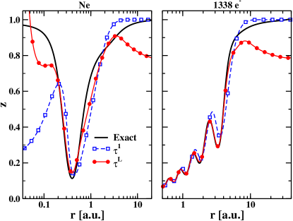
Figure 3: Plot of $z=\tau^{\text{W}}/\tau$ for the Ne atom and a non relativistic atom with 1338 electrons, as computed with the exact $\tau$, $\tau=\tau^{1}$, and $\tau=\tau^{L}$.

Appendix A Behavior of $\tau^{revAPBEk}+(20/9)\tau^{TF}q$ in the tail of the density

Let consider a spherical atom, where the density decays exponentially as $\rho=Ae^{-\alpha r}$, with $r$ being the radial distance from the nucleus. In this case,

$$\frac{s^{2}}{q}=\frac{\alpha r}{\alpha r-2}\xrightarrow[r\rightarrow\infty]{}1.$$ (39)

A similar expression can also be obtained for a Gaussian decaying density $n=Ae^{-\alpha r^{2}}$

$$\frac{s^{2}}{q}=\frac{2\alpha r^{2}}{2\alpha r^{2}-3}\xrightarrow[r\rightarrow\infty]{}1.$$ (40)

Thus, in the tail of the density $q\approx s^{2}$, and so

$$\tau^{revAPBEk}+\frac{20}{9}\tau^{TF}q\xrightarrow[r\rightarrow\infty]{}\frac{20}{9}\tau^{TF}s^{2},$$ (41)

where we considered that the revAPBEK enhancement factor asymptotically behaves as a constant. Finally we find

$$z\xrightarrow[r\rightarrow\infty]{}\frac{5/3}{20/9}=\frac{3}{4}.$$ (42)

Note, however, that this behavior is valid only at large distances that are not important in practical calculations, see Fig. 3. In valence and close tail regions $z$ is instead very close to the exact one, as shown in Fig. 1 and Fig. 3.

References

- Cortona (1991) P. Cortona, Phys. Rev. B 44, 8454 (1991).
- Wesolowski and Weber (1996) T. A. Wesolowski and J. Weber, Chem. Phys. Lett. 248, 71 (1996).
- Wesolowski (2006) T. A. Wesolowski, in Chemistry: Reviews of Current Trends, edited by J. Leszczynski (World Scientific: Singapore, 2006, Singapore, 2006), vol. 10, pp. 1–82.
- Neugebauer (2010) J. Neugebauer, Phys. Rep. 489, 1 (2010).
- Jacob and Neugebauer (2014) C. R. Jacob and J. Neugebauer, Wiley Interdisciplinary Reviews: Computational Molecular Science 4, 325 (2014).
- Krishtal et al. (2015) A. Krishtal, D. Sinha, A. Genova, and M. Pavanello, J. Phys. Cond. Matt. (2015), in press.
- Hohenberg and Kohn (1964) P. Hohenberg and W. Kohn, Phys. Rev. 136, B864 (1964).
- Kohn and Sham (1965) W. Kohn and L. J. Sham, Phys. Rev. 140, A1133 (1965).
- Wesolowski et al. (1996) T. A. Wesolowski, H. Chermette, and J. Weber, J. Chem. Phys. 105, 9182 (1996).
- Wesolowski (1997) T. A. Wesolowski, J. Chem. Phys. 106, 8516 (1997).
- Wesołowski et al. (1998) T. A. Wesołowski, Y. Ellinger, and J. Weber, J. Chem. Phys. 108 (1998).
- Wesolowski and Tran (2003) T. A. Wesolowski and F. Tran, J. Chem. Phys. 118, 2072 (2003).
- Kevorkyants et al. (2006) R. Kevorkyants, M. Dulak, and T. A. Wesolowski, J. Chem. Phys. 124, 024104 (2006).
- Dulak and Wesolowski (2007) M. Dulak and T. A. Wesolowski, J. Molec. Model. 13, 631 (2007).
- Dułak et al. (2007) M. Dułak, J. W. Kamiński, and T. A. Wesołowski, J. Chem. Theory Comput. 3, 735 (2007).
- Garcia Lastra et al. (2008) J. M. Garcia Lastra, J. W. Kaminski, and T. A. Wesolowski, J. Chem. Phys. 129, 074107 (2008).
- Götz et al. (2009) A. W. Götz, S. M. Beyhan, and L. Visscher, J. Chem. Theory Comput. 5, 3161 (2009).
- Fradelos and Wesolowski (2011) G. Fradelos and T. A. Wesolowski, J. Chem. Theory Comput. 7, 213 (2011).
- Constantin et al. (2011a) L. A. Constantin, E. Fabiano, S. Laricchia, and F. Della Sala, Phys. Rev. Lett. 106, 186406 (2011a).
- Laricchia et al. (2011a) S. Laricchia, E. Fabiano, L. A. Constantin, and F. Della Sala, J. Chem. Theory Comput. 7, 2439 (2011a).
- Laricchia et al. (2011b) S. Laricchia, E. Fabiano, and F. Della Sala, Chem. Phys. Lett. 518, 114 (2011b).
- Laricchia et al. (2012) S. Laricchia, E. Fabiano, and F. Della Sala, J. Chem. Phys. 137, 014102 (2012).
- Fabiano et al. (2014a) E. Fabiano, S. Laricchia, and F. Della Sala, J. Chem. Phys. 140, 114101 (2014a).
- Laricchia et al. (2013) S. Laricchia, E. Fabiano, and F. Della Sala, J. Chem. Phys. 138, 124112 (2013).
- Laricchia et al. (2014) S. Laricchia, L. A. Constantin, E. Fabiano, and F. Della Sala, J. Chem. Theory Comput. 10, 164 (2014).
- Schluns et al. (2015) D. Schluns, K. Klahr, C. Muck-Lichtenfeld, L. Visscher, and J. Neugebauer, Phys. Chem. Chem. Phys. (2015), in press.
- Kevorkyants et al. (2014) R. Kevorkyants, H. Eshuis, and M. Pavanello, J. Chem. Phys. 141, 044127 (2014).
- Jacob and Visscher (2008) C. R. Jacob and L. Visscher, J. Chem. Phys. 128, 155102 (2008).
- Fux et al. (2008) S. Fux, K. Kiewisch, C. R. Jacob, J. Neugebauer, and M. Reiher, Chem. Phys. Lett. 461, 353 (2008).
- Beyhan et al. (2010) S. M. Beyhan, A. W. Götz, C. R. Jacob, and L. Visscher, J. Chem. Phys. 132, 044114 (2010).
- Fux et al. (2010) S. Fux, C. R. Jacob, J. Neugebauer, L. Visscher, and M. Reiher, J. Chem. Phys. 132, 164101 (2010).
- Wesolowski and Warshel (1993) T. A. Wesolowski and A. Warshel, J. Phys. Chem. 97, 8050 (1993).
- Hodak et al. (2008) M. Hodak, W. Lu, and J. Bernholc, J. Chem. Phys. 128, 014101 (2008).
- Neugebauer et al. (2005a) J. Neugebauer, M. J. Louwerse, E. J. Baerends, and T. A. Wesolowski, J. Chem. Phys. 122, 094115 (2005a).
- Jacob et al. (2006) C. R. Jacob, J. Neugebauer, L. Jensen, and L. Visscher, Phys. Chem. Chem. Phys. 8, 2349 (2006).
- Neugebauer et al. (2005b) J. Neugebauer, M. J. Louwerse, P. Belanzoni, T. A. Wesolowski, and E. J. Baerends, J. Chem. Phys. 123, 114101 (2005b).
- Kaminski et al. (2010) J. W. Kaminski, S. Gusarov, T. A. Wesolowski, and A. Kovalenko, J. Phys. Chem. A 114, 6082 (2010).
- Kiewisch et al. (2013) K. Kiewisch, C. R. Jacob, and L. Visscher, J. Chem. Theory Comput. 9, 2425 (2013).
- Tran et al. (2002) F. Tran, J. Weber, T. A. Wesołowski, F. Cheikh, Y. Ellinger, and F. Pauzat, J. Phys. Chem. B 106, 8689 (2002).
- Lembarki and Chermette (1994) A. Lembarki and H. Chermette, Phys. Rev. A 50, 5328 (1994).
- Thakkar (1992) A. J. Thakkar, Phys. Rev. A 46, 6920 (1992).
- Lee et al. (1991) H. Lee, C. Lee, and R. G. Parr, Phys. Rev. A 44, 768 (1991).
- Tran and Wesolowski (2013) F. Tran and T. A. Wesolowski, in Recent Progress in Orbital-free Density Functional Theory, edited by T. A. Wesolowsky and Y. A. Wang (World Scientific, Singapore, 2013), pp. 429–442.
- Laricchia et al. (2010) S. Laricchia, E. Fabiano, and F. Della Sala, J. Chem. Phys. 133, 164111 (2010).
- Wesołowski (2008) T. A. Wesołowski, Phys. Rev. A 77, 012504 (2008).
- Jacob et al. (2005) C. R. Jacob, T. A. Wesolowski, and L. Visscher, J. Chem. Phys. 123, 174104 (2005).
- Pernal and Wesolowski (2009) K. Pernal and T. Wesolowski, Int. Jou. Quant. Chem. 109, 2520 (2009).
- Tao et al. (2003) J. Tao, J. P. Perdew, V. N. Staroverov, and G. E. Scuseria, Phys. Rev. Lett. 91, 146401 (2003).
- Perdew et al. (2009) J. P. Perdew, A. Ruzsinszky, G. I. Csonka, L. A. Constantin, and J. Sun, Phys. Rev. Lett. 103, 026403 (2009).
- Constantin et al. (2011b) L. A. Constantin, L. Chiodo, E. Fabiano, I. Bodrenko, and F. Della Sala, Phys. Rev. B 84, 045126 (2011b).
- Constantin et al. (2012) L. A. Constantin, E. Fabiano, and F. Della Sala, Phys. Rev. B 86, 035130 (2012).
- Constantin et al. (2013a) L. A. Constantin, E. Fabiano, and F. Della Sala, J. Chem. Theory Comput. 9, 2256 (2013a).
- Van Voorhis and Scuseria (1998) T. Van Voorhis and G. E. Scuseria, J. Chem. Phys. 109, 400 (1998).
- Schmider and Becke (1998) H. L. Schmider and A. D. Becke, J. Chem. Phys. 109, 8188 (1998).
- Zhao and Truhlar (2006) Y. Zhao and D. G. Truhlar, J. Chem. Phys. 125, 194101 (2006).
- Peverati and Truhlar (2012) R. Peverati and D. G. Truhlar, J. Phys. Chem. Lett. 3, 117 (2012).
- Ruzsinszky et al. (2012) A. Ruzsinszky, J. Sun, B. Xiao, and G. I. Csonka, J. Chem. Theory Comput. 8, 2078 (2012).
- Sun et al. (2012) J. Sun, B. Xiao, and A. Ruzsinszky, J. Chem. Phys. 137, 051101 (2012).
- Sun et al. (2013a) J. Sun, R. Haunschild, B. Xiao, I. W. Bulik, G. E. Scuseria, and J. P. Perdew, J. Chem. Phys. 138, 044113 (2013a).
- Sun et al. (2015) J. Sun, J. P. Perdew, and A. Ruzsinszky, Proc. Nat. Acad. Sci. 112, 685 (2015).
- Wellendorff et al. (2014) J. Wellendorff, K. T. Lundgaard, K. W. Jacobsen, and T. Bligaard, J. Chem. Phys. 140, 144107 (2014).
- Mardirossian and Head-Gordon (2015) N. Mardirossian and M. Head-Gordon, J. Chem. Phys. 142, 074111 (2015).
- Constantin et al. (2013b) L. A. Constantin, E. Fabiano, and F. Della Sala, Phys. Rev. B 88, 125112 (2013b).
- Della Sala et al. (2015) F. Della Sala, E. Fabiano, and L. A. Constantin, Phys. Rev. B 91, 035126 (2015).
- Xiao et al. (2013) B. Xiao, J. Sun, A. Ruzsinszky, J. Feng, R. Haunschild, G. E. Scuseria, and J. P. Perdew, Phys. Rev. B 88, 184103 (2013).
- Sun et al. (2013b) J. Sun, B. Xiao, Y. Fang, R. Haunschild, P. Hao, A. Ruzsinszky, G. I. Csonka, G. E. Scuseria, and J. P. Perdew, Phys. Rev. Lett. 111, 106401 (2013b).
- Staroverov et al. (2004) V. N. Staroverov, G. E. Scuseria, J. Tao, and J. P. Perdew, Phys. Rev. B 69, 075102 (2004).
- Adamo et al. (2000) C. Adamo, M. Ernzerhof, and G. E. Scuseria, J. Chem. Phys. 112, 2643 (2000).
- Riley et al. (2007) K. E. Riley, B. T. Op’t Holt, and K. M. Merz, J. Chem. Theory Comput. 3, 407 (2007).
- Andersen et al. (2012) M. Andersen, L. Hornekær, and B. Hammer, Phys. Rev. B 86, 085405 (2012).
- Luo et al. (2012) S. Luo, Y. Zhao, and D. G. Truhlar, J. Phys. Chem. Lett. 3, 2975 (2012).
- Sun et al. (2011) J. Sun, M. Marsman, A. Ruzsinszky, G. Kresse, and J. P. Perdew, Phys. Rev. B 83, 121410 (2011).
- Hao et al. (2013) P. Hao, J. Sun, B. Xiao, A. Ruzsinszky, G. I. Csonka, J. Tao, S. Glindmeyer, and J. P. Perdew, J. Chem. Theory Comput. 9, 355 (2013).
- Fabiano et al. (2014b) E. Fabiano, L. A. Constantin, and F. Della Sala, J. Chem. Theory Comput. 10, 3151 (2014b).
- Nazarov and Vignale (2011) V. U. Nazarov and G. Vignale, Phys. Rev. Lett. 107, 216402 (2011).
- Arbuznikov and Kaupp (2003a) A. V. Arbuznikov and M. Kaupp, Chem. Phys. Lett. 381, 495 (2003a).
- Seidl et al. (1996) A. Seidl, A. Görling, P. Vogl, J. A. Majewski, and M. Levy, Phys. Rev. B 53, 3764 (1996).
- Gritsenko (2013) O. Gritsenko, in Recent Progress in Orbital-free Density Functional Theory, edited by T. A. Wesolowsky and Y. A. Wang (World Scientific, Singapore, 2013), pp. 355–365.
- Arbuznikov and Kaupp (2003b) A. V. Arbuznikov and M. Kaupp, Chem. Phys. Lett. 381, 495 (2003b).
- Arbuznikov et al. (2002) A. V. Arbuznikov, M. Kaupp, V. G. Malkin, R. Reviakine, and O. L. Malkina, Phys. Chem. Chem. Phys. 4, 5467 (2002).
- Humbert-Droz et al. (2013) M. Humbert-Droz, X. Zhou, S. Shedge, and T. Wesolowski, Theor. Chem. Acc. 133, 1405 (2013).
- Nafziger and Wasserman (2014) J. Nafziger and A. Wasserman, J. Phys. Chem. A 118, 7623 (2014).
- Zhao et al. (1995) Q. Zhao, R. C. Morrison, and R. G. Parr, Phys. Rev. A 50, 238 (1995).
- Wu and Yang (2003) Q. Wu and W. Yang, J. Chem. Phys. 118, 2498 (2003).
- de Silva and Wesolowski (2012) P. de Silva and T. A. Wesolowski, Phys. Rev. A 85, 032518 (2012).
- Roncero et al. (2008) O. Roncero, M. P. de Lara-Castells, P. Villarreal, F. Flores, J. Ortega, M. Paniagua, and A. Aguado, J. Chem. Phys. 129, 184104 (2008).
- Roncero et al. (2009) O. Roncero, A. Zanchet, P. Villarreal, and A. Aguado, J. Chem. Phys. 131, 234110 (2009).
- Goodpaster et al. (2010) J. D. Goodpaster, N. Ananth, F. R. Manby, and T. F. Miller III, J. Chem. Phys. 133, 084103 (2010).
- Goodpaster et al. (2011) J. D. Goodpaster, T. A. Barnes, and T. F. Miller III, J. Chem. Phys. 134, 164108 (2011).
- Kümmel and Kronik (2008) S. Kümmel and L. Kronik, Rev. Mod. Phys. 80, 3 (2008).
- Jacob (2011) C. R. Jacob, J. Chem. Phys. 135, 244102 (2011).
- Heßelmann et al. (2007) A. Heßelmann, A. W. Götz, F. Della Sala, F. Manby, and A. Görling, J. Chem. Phys. 127, 054102 (2007).
- Staroverov et al. (2006) V. N. Staroverov, G. E. Scuseria, and E. R. Davidson, J. Chem. Phys. 124, 141103 (2006).
- Heaton-Burgess et al. (2007) T. Heaton-Burgess, F. A. Bulat, and W. Yang, Phys. Rev. Lett. 98, 256401 (2007).
- Yang et al. (1986) W. Yang, R. G. Parr, and C. Lee, Phys. Rev. A 34, 4586 (1986).
- García-Aldea and Alvarellos (2007) D. García-Aldea and J. E. Alvarellos, J. Chem. Phys. 127, 144109 (2007).
- Ayers et al. (2002) P. W. Ayers, R. G. Parr, and A. Nagy, Int. Jou. Quant. Chem. 90, 309 (2002).
- Thomas (1926) L. H. Thomas, Proc. Cambridge Phil. Soc. 23, 542 (1926).
- Fermi (1928) E. Fermi, Rend. Accad. Naz. Lincei 48, 73 (1928).
- Fermi (1927) E. Fermi, Z. Phys. 6, 602 (1927).
- von Weizsäcker (1935) C. F. von Weizsäcker, Z. Phys. A 96, 431 (1935).
- Della Sala et al. (2015) F. Della Sala, E. Fabiano, and L. A. Constantin, Phys. Rev. B 91, 035126 (2015).
- Brack et al. (1976) M. Brack, B. Jennings, and Y. Chu, Phys. Lett. B 65, 1 (1976).
- Kirzhnits (1957) D. A. Kirzhnits, Sov. Phys. JETP 5, 64 (1957).
- Lee et al. (2009) D. Lee, L. A. Constantin, J. P. Perdew, and K. Burke, J. Chem. Phys. 130, 034107 (2009).
- Perdew et al. (1996a) J. P. Perdew, K. Burke, and M. Ernzerhof, Phys. Rev. Lett. 77, 3865 (1996a).
- Adamo and Barone (1999) C. Adamo and V. Barone, J. Chem. Phys. 110, 6158 (1999).
- Perdew et al. (1996b) J. P. Perdew, M. Ernzerhof, and K. Burke, J. Chem. Phys. 105, 9982 (1996b).
- Weigend and Ahlrichs (2005) F. Weigend and R. Ahlrichs, Phys. Chem. Chem. Phys. 7, 3297 (2005).
- Rappoport and Furche (2010) D. Rappoport and F. Furche, J. Chem. Phys. 133, 134105 (2010).
- (111) TURBOMOLE V6.2, 2009, a development of University of Karlsruhe and Forschungszentrum Karlsruhe GmbH, 1989-2007, TURBOMOLE GmbH, since 2007; available from http://www.turbomole.com.
- Zhao and Truhlar (2005a) Y. Zhao and D. G. Truhlar, J. Phys. Chem. A 109, 5656 (2005a).
- Zhao and Truhlar (2005b) Y. Zhao and D. G. Truhlar, J. Chem. Theory Comput. 1, 415 (2005b).