The aperiodic X-ray variability of the accreting millisecond pulsar SAX J1808.4–3658

Abstract

We have studied the aperiodic variability of the 401 Hz accreting millisecond X-ray pulsar SAX J1808.4–3658 using the complete data set collected with the Rossi X-ray Timing Explorer over 14 years of observation. The source shows a number of exceptional aperiodic timing phenomena that are observed against a backdrop of timing properties that show consistent trends in all five observed outbursts and closely resemble those of other atoll sources. We performed a detailed study of the enigmatic $\sim$410 Hz QPO, which has only been observed in SAX J1808.4–3658. We find that it appears only when the upper kHz QPO frequency is less than the 401 Hz spin frequency. The difference between the $\sim$410 Hz QPO frequency and the spin frequency follows a similar frequency correlation as the low frequency power spectral components, suggesting that the $\sim$410 Hz QPO is a retrograde beat against the spin frequency of a rotational phenomenon in the 9 Hz range. Comparing this 9 Hz beat feature with the Low-Frequency QPO in SAX J1808.4–3658 and other neutron star sources, we conclude that these two might be part of the same basic phenomenon. We suggest that they might be caused by retrograde precession due to a combination of relativistic, classical and magnetic torques. Additionally we present two new measurements of the lower kHz QPO, allowing us, for the first time, to measure the frequency evolution of the twin kHz QPOs in this source. The twin kHz QPOs are seen to move together over 150 Hz, maintaining a centroid frequency separation of $(0.446\pm 0.009)\nu_{\text{spin}}$.

1. Introduction

The transient X-ray source SAX J1808.4–3658 (SAX J1808) was discovered with the BeppoSax satellite in September 1996 (in ’t Zand et al., 1998). It remained in quiescence for 1.6 yr after the discovery, until the Rossi X-ray Timing Explorer (RXTE) detected renewed X-ray activity with the Proportional Counter Array (Marshall et al., 1998). The initial RXTE observations revealed coherent pulsations at 401 Hz, making SAX J1808 the first known accreting millisecond X-ray pulsar (AMXP) (Wijnands & van der Klis, 1998a).

From extrapolating the recurrence time between the 1996 and 1998 outbursts, SAX J1808 was expected to show a new cycle of activity around November 1999. Unfortunately, Solar constraints prevented observations until late January 2000, at which time SAX J1808 was observed to be in a low luminosity state at roughly a tenth of the typical flux of the 1998 outburst (van der Klis et al., 2000). It is generally assumed that the main outburst occurred when the Solar constraints prevented observation (Wijnands et al., 2001). The low luminosity state persisted for $\sim 114$ days (Wijnands et al., 2001), showing dramatic changes in luminosity. On a timescale of $\sim$5 days the luminosity would drop below a detection limit of $\sim 10^{32}$ erg s^-1 and then increase again to $\sim 10^{35}$ erg s^-1. During these episodes of increased emission the 401 Hz pulsations were detected along with a sporadic strong modulation at about 1 Hz (van der Klis et al., 2000). Campana et al. (2008) proposed that the 5-day episodic variations of luminosity were caused by an intermittently active propellor effect (Illarionov & Sunyaev, 1975), periodically inhibiting accretion onto the neutron star. The 1 Hz flaring remained unique to SAX J1808 until a similar feature was discovered in the AMXP NGC 6440 X-2 (Patruno et al., 2010; Patruno & D’Angelo, 2013).

The fourth outburst of SAX J1808 was detected in October 2002, some 2.8 yr after the 2000 outburst, triggering an extensive monitoring campaign with RXTE. Twin kHz quasi-periodic oscillations (QPOs) were detected early in the outburst (Wijnands et al., 2003), for the first time in a source for which the spin frequency was precisely known. An additional QPO was unexpectedly detected at 410 Hz, which so far is unique to SAX J1808 and whose nature remains a mystery. After the main outburst, which lasted several weeks, the source entered a low luminosity state showing the same $\sim$5 day episodes of increased emission and 1 Hz flaring seen in 2000 (Wijnands, 2004).

Since its 2002 outburst, SAX J1808 has been observed in outburst another three times; in 2005, 2008 and 2011. For both the 2005 and 2008 outbursts a low-luminosity prolonged outburst tail was observed, again showing luminosity variations on a $\sim 5$ day timescale. During these episodes the 1 Hz flaring was again observed in 2005 but not in 2008 (Patruno et al., 2009). Observations of the 2011 outburst were cut short by Solar constraints, such that only the onset of the low-luminosity outburst tail was seen, where again, no 1 Hz flaring was detected (Patruno et al., 2012). The 2008 and 2011 outbursts were later found to show a 1–5 Hz flaring which shares many of the characteristics of the 1 Hz flaring, but occurred at luminosities an order of magnitude higher, near the peak of the outburst (Bult & van der Klis, 2014).

SAX J1808 showed several thermonuclear X-ray bursts in each outburst. Using the X-ray bursts of the 1998, 2002 and 2005 outbursts Galloway & Cumming (2006) derived a distance estimate of $3.5\pm 0.1$ kpc.

The literature contains a large body of work on the coherent pulsations of SAX J1808 (Wijnands & van der Klis, 1998a; Poutanen & Gierliński, 2003; Burderi et al., 2006; Hartman et al., 2008; Leahy et al., 2008; Hartman et al., 2009; Ibragimov & Poutanen, 2009; Patruno et al., 2012). The study of the stochastic variability of SAX J1808, on the other hand, remains incomplete, with all work constrained to the earlier outbursts. Specifically, Wijnands & van der Klis (1998b) studied the broadband power spectrum of the 1998 outburst and Menna et al. (2003) considered the coupling between the broad band noise and the coherent pulsations. The 2002 outburst power spectrum was studied by Wijnands et al. (2003), but only the high frequency region, in the context of the kHz QPOs. A more general analysis of the 1998 and 2002 outbursts was done by van Straaten et al. (2005), who compared the timing behavior of AMXPs with non-pulsating low-mass X-ray binaries. The stochastic variability of the 2005, 2008 and 2011 outbursts remains unaddressed.

With the demise of RXTE, its 14 year monitoring campaign of SAX J1808 has now been completed. We use this remarkable dataset to provide a complete overview of the stochastic time variability of SAX J1808. In this work we analyze all outbursts in a consistent approach, but do not consider the low luminosity outburst tail, which has been studied in-depth by Patruno et al. (2009). We provide the first in-depth analysis of the broadband power spectra of the 2005, 2008 and 2011 outbursts and characterize the rich variability phenomenology observed in this accreting millisecond X-ray pulsar.

2. Data Reduction

We used all RXTE pointed observations of SAX J1808’s outbursts (see Table 1 for ObsIDs), selecting only observations with stable pointing, source elevation above 10^∘ and pointing offset less than 0.02^∘.

Table 1 Interval Listing

Interval	State	Start MJD	ObsIDs
1998 Outburst
1	IS	50914.9	A-01-03S
2	EIS	50919.8	A-03-00
3	EIS	50920.1	A-04-00
4	EIS	50921.3	A-05-00
5	EIS	50921.5	A-06-01
6	EIS	50921.7	A-06-000
7	EIS	50921.9	A-06-00
8	EIS	50923.9	A-07-00
9	EIS	50926.8	A-08-00
10	EIS	50927.7	A-09-01, A-09-02
11	EIS	50928.6	A-09-03, A-09-04
12	EIS	50929.8	A-09-00
13	EIS	50930.6	A-10-02, A-10-01, A-10-00
2002 Outburst
1	IS	52562.1	B-03-04-00
2	LLB	52562.3	B-01-01-000
3	LLB	52563.1	B-01-01-03, B-01-01-04
4	LLB	52563.4	B-01-01-01
5	LLB	52564.3	B-01-01-020, B-01-01-02
6	IS	52565.0	B-01-02-01, B-01-02-000, B-01-02-00
7	IS	52566.0	B-01-02-02, B-01-02-03, B-01-02-04
8	IS	52567.1	B-01-02-05, B-01-02-06, B-01-02-07
9	IS	52568.1	B-01-02-10, B-01-02-08
10	IS	52569.0	B-01-02-20
11	IS	52569.2	B-01-02-09
12	IS	52569.4	B-01-02-19, B-01-02-23
13	IS	52570.0	B-01-02-21, B-01-02-11
14	IS	52570.4	B-01-02-18, B-01-02-12, B-01-02-22
15	IS	52571.0	B-01-02-13, B-01-02-15, B-01-02-14, B-01-02-16
16	IS	52572.0	B-01-02-17, B-01-03-00, B-01-03-04, B-01-03-05
17	IS	52572.2	B-01-03-000
18	IS	52572.9	B-01-03-06, B-01-03-07, B-01-03-010, B-01-03-01
19	IS	52573.4	B-01-03-08, B-01-03-09, B-01-03-10, B-01-03-11, B-01-03-12, B-01-03-13
20	IS	52574.1	B-01-03-02
21	IS	52574.8	B-01-03-14, B-01-03-03, B-03-05-00, B-02-01-04
22	IS	52577.1	B-02-01-000, B-02-01-00
2005 Outburst
1	IS	53523.0	C-01-01
2	IS	53523.5	C-01-02, C-01-03, C-01-04, C-01-05, C-02-00
3	IS	53524.9	C-02-01
4	IS	53525.8	C-02-02
5	IS	53526.8	C-02-030
6	IS	53527.0	C-02-03
7	LLB	53527.8	C-02-04, C-02-05, C-02-06
8	IS	53530.8	C-02-08
9	IS	53531.3	C-03-03, C-03-02, C-03-00, C-03-01
10	IS	53533.6	C-03-05, C-03-04, C-03-07, C-03-08
11	IS	53535.7	C-03-06, C-03-09, C-03-11, C-03-10
2008 Outburst
1	IS	54731.9	D-01-01, D-01-00, D-01-02
2	IS	54732.7	D-01-080, D-01-08, D-01-03
3	IS	54733.7	D-01-04, D-01-07, D-01-06, D-01-05, D-01-10, D-02-00, D-02-01
4	IS	54736.5	D-02-05, D-02-06, D-02-03, D-02-04
5	IS/F	54739.4	D-02-07, D-02-09, D-02-02, D-02-08
6	IS	54742.5	D-03-00, D-03-01, D-03-08, D-03-02
7	IS	54745.5	D-03-03, D-03-10, D-03-05, D-03-04
2011 Outburst
1	IS/F	55869.9	E-01-01, E-01-00
2	IS/F	55871.1	E-01-02
3	IS/F	55872.0	E-01-03, E-01-04
4	LLB/F	55872.9	E-01-05, E-01-06
5	LLB	55874.0	E-01-070, E-01-07
6	IS	55875.2	E-01-08, E-01-09, E-02-00
7	IS	55877.0	E-02-01, E-02-02
8	IS	55878.0	E-02-03, E-02-04
9	EIS	55879.0	E-02-05, E-02-06, E-02-07, E-02-08
10	EIS	55881.3	E-02-09, E-02-10, E-03-00, E-03-01, E-03-04

Note. — RXTE ObsIDs grouped together in intervals for all outbursts. ObsIDs are chronologically ordered from left to right and top to bottom. Source states are abbreviated as: EIS - extreme island state; IS - island state; LLB - lower-left banana, F - low luminosity flaring present. A = ‘30411-01’; B = ‘70080’, C = ‘91056-01’, D = ‘93027-01’, E = ‘96027-01’.

Using the Standard-2 data we created Crab normalized 2–16 keV light curves. We also calculated the Crab normalized soft color as the count rate in the 3.5–6.0 keV band divided by the count rate in the 2.0–3.5 keV band. Similarly, the Crab normalized hard color is calculated by dividing the 9.7–16 keV band count rate by the count rate in the 6.0–9.7 keV band (see e.g. van Straaten et al. 2003, for the detailed procedure).

The timing analysis was done using high time resolution (122 $\mu$s) Event and GoodXenon data, selecting all events in the 2–20 keV energy band. Data obtained in GoodXenon mode were binned to 122 $\mu$s prior to further analysis. Fourier transforms were calculated using 256 s segments at full time resolution, yielding power spectra with a frequency resolution of $\sim$0.004 Hz and a Nyquist frequency of 4096 Hz. No background subtraction or dead-time correction was applied prior to the Fourier transform. The power spectra were calculated using the standard Leahy normalization (Leahy et al., 1983). Following the method of Klein-Wolt et al. (2004) we inspected the high frequency region ($>1500$ Hz) for anomalous features. Since none were found we subtracted a Poisson noise power spectrum calculated using the analytical formula of Zhang et al. (1995) and shifted to fit the $>1500$ Hz power. All power spectra were averaged per ObsID. If necessary, multiple consecutive ObsIDs were averaged into intervals to improve statistics, but only if the power spectra showed similar morphology and the corresponding colors and intensities were consistent with being the same. Details of the intervals used are given in Table 1. Finally we estimated the background count rate using the ftool pcabackest and used it to renormalize the power spectra to units of source fractional rms squared per Hz (van der Klis, 1995).

The power spectra are described in terms of a sum of Lorentzian profiles (see e.g. Nowak 2000; Belloni et al. 2002). Each profile, $L(\nu|\nu_{\max},Q,r)$, is a function of Fourier frequency $\nu$ and determined by three parameters: the characteristic frequency $\nu_{\max}=\sqrt{\nu_{0}^{2}+(\mbox{FWHM}/2)^{2}}$, the quality factor $Q=\nu_{0}/\mbox{FWHM}$ and its fractional rms amplitude squared $r^{2}=P=\int_{0}^{\infty}L(\nu)d\nu$. Here $\nu_{0}$ is the Lorentzian centroid frequency and FWHM the full-width-at-half-maximum. A feature is called a QPO if $Q>2$. Features with $Q<2$ are called noise components. We consider a component to be significant if the ratio of the integrated power to its single trial negative error is greater than three; $P/{\sigma_{P}}\geq 3$. Boundary cases with $P\simeq 3\sigma_{P}$ for which we deviate from this rule are explicitly discussed in Section 4.

In the 2008 and 2011 outbursts we previously found a broad noise component centered at 1–5 Hz (Bult & van der Klis, 2014), which we called high luminosity flaring. This flaring component cannot be fitted with a Lorentzian profile, but instead is well described by a Schechter function, which is a power-law with an exponential cut-off, $S(\nu)\propto\nu^{-\alpha}e^{-\nu/\nu_{\text{cut}}}$ (Hasinger & van der Klis, 1989; Dotani et al., 1989), with power law index $\alpha$ and cut-off frequency $\nu_{\text{cut}}$. To compare the Schechter function with Lorentzian components, and by analogy to the definitions used for Lorentzian components, we define the Schechter “centroid” frequency, $\nu_{0}=-\alpha\nu_{\text{cut}}$, as the frequency of maximum power in $S(\nu)$. Alternatively, we can define a characteristic frequency, $\nu_{\max}=(1-\alpha)\nu_{\text{cut}}$, as the frequency of the maximum in $\nu S(\nu)$.

3. Source State Identification

Atoll sources are named after the shape they trace out in the color-color diagram (Hasinger & van der Klis, 1989; van der Klis, 2006). At high luminosities they exhibit a banana shaped pattern, which is divided into three regions corresponding to three source states (upper, lower and lower-left banana). At lower luminosities the hard color increases and the observations cluster in the island state. In the hardest, lowest luminosity states a change in variability distinguishes another source state; the extreme island state. Depending on the source state, atoll sources show a different number of power spectral features and have a different morphology (see van der Klis 2006 for a detailed overview).

SAX J1808 is a low luminosity atoll source (van Straaten et al., 2005) and has shown only three source states: the extreme island state, the island state and the lower-left banana. We discuss the power spectral shapes relevant to these source states.

In the extreme island state three to four broad Lorentzians are needed to fit the power spectrum. The components with the lowest and second lowest characteristic frequencies are respectively called the break ($b$) and hump ($h$) Lorentzians (Belloni et al., 2002). The highest frequency component is usually found at 100–200 Hz and is identified as “$u$” to represent the widely held idea that this component evolves into the upper kHz QPO found in the island state and the lower-left banana (Psaltis et al., 1999). An additional component is usually present between the upper kHz and hump Lorentzian, which is proposed to evolve into the lower kHz QPO (Psaltis et al., 1999), but that identification is debated (van Straaten et al., 2003). In this work we follow van Straaten et al. (2005) and label this feature as a separate “${\ell}\text{ow}$” component. The relation between the ${\ell}\text{ow}$ component and the lower kHz QPO is further discussed in section 5.1.2

In the island state three or four Lorentzian profiles are needed. These components tend to be less broad, while covering a higher frequency range with respect to the Lorentzians seen in the extreme island state. The lowest frequency noise components are again called the break and hump Lorentzians. The highest frequency component is now a QPO, and identified as the upper kHz QPO (Wijnands et al., 2003). Often an additional Lorentzian is needed at $\nu_{\rm max}\sim 100-200$ Hz, which is called the hectohertz (hHz) component (Ford & van der Klis, 1998; van Straaten et al., 2002). This component is usually observed as a broad noise component with a quality factor below 0.5. Occasionally it becomes more peaked, but it always has $Q\lesssim 2$. A characteristic property of the hHz component is that it does not show a systematic trend in frequency. It stays roughly constant in the hectohertz range. A ${\ell}\text{ow}$ component is not usually observed in the island state, but given their similar frequencies, the ${\ell}\text{ow}$ and hHz components may be difficult to disentangle. We simply always label the noise component below the upper kHz QPO as the hHz component and discuss this issue further in section 5.1.3.

In the lower-left banana the power spectra show a complex morphology and can require up to seven different Lorentzians. In contrast to the two island states, the lower-left banana may show two breaks in the broad band noise, “$b$” and “$b2$”, with ${b2}$ being the lower frequency component. As in the island state, higher frequency features are called the hump and hectohertz components. Finally, at the highest frequencies a lower ($\ell$) and upper ($u$) kHz QPO is seen. If both kHz QPOs are detected in SAX J1808, the upper kHz QPO is always the most prominent feature, so if only one QPO is present, it is identified as the upper kHz QPO (Wijnands et al., 2003; van Straaten et al., 2005). Because the lower kHz QPO always appear as a very sharp, weak QPO it can be easily distinguished from the much broader hHz component that may be present at a lower frequency.

In some atoll sources the hump feature occasionally shows two discernible peaks, or a complex morphology requiring two Lorentzian profiles for an acceptable fit. In such cases the narrow Lorentzian is called the Low-Frequency (LF) component, while the broader Lorentzian is called the hump ($h$) component. In SAX J1808 the two components are sometimes both narrow QPOs, in which case we call the lower frequency component LF and the higher frequency component the hump.

Following Belloni et al. (2002) we refer to each Lorentzian profile as $L_{i}$, where subscript $i=\{b2,b,\text{LF},h,{\ell}\text{ow},\text{hHz},\ell,u\}$ represents the name of the specific component (e.g. $L_{b}$ refers to the break component). We may further use $\nu_{i}$ to refer to characteristic frequency and $\nu_{0,i}$ for the centroid frequency. Similarly, the quality factor and fractional rms are referred to as $Q_{i}$ and $r_{i}$.

4. Results

We briefly discuss the timing and color evolution of SAX J1808 for each individual outburst. We make use of Figure 1, which shows the 2–16 keV light curves, and the soft and hard color evolution for all outbursts. Additionally, we refer to Figure 2, which shows a sample of representative power spectra for each outburst, and Tables 2, 4, 4 and 5 which list the full set of fit parameters obtained for SAX J1808.

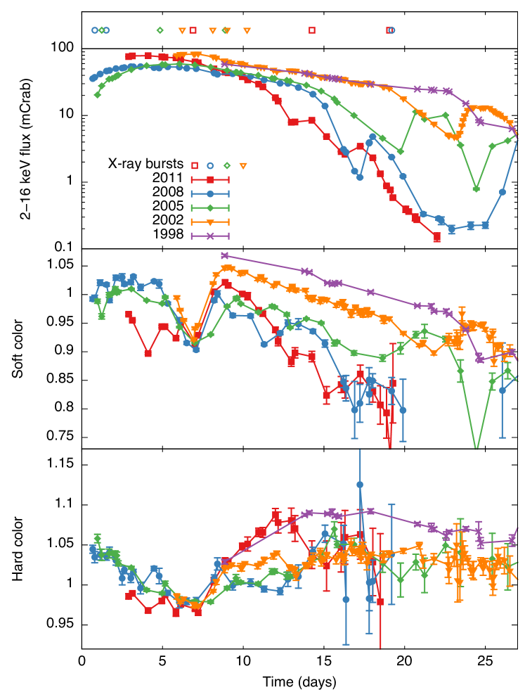
Figure 1.— Evolution of the outbursts of SAX J1808. The top panel gives the times of type I X-ray bursts. The second panel gives the 2–16 keV light curves, while the third and fourth panel give the evolution of the soft and hard colors, respectively. Color measurements with large uncertainties have been omitted for clarity. Each light curve has been shifted in time by: 2011 MJD 55867.03; 2008 MJD 54731.20; 2005 MJD 53521.79; 2002 MJD 52556.19; and 1998 MJD 50906.03, such that their color minima approximately match on day 7.0. Each point in this figure corresponds to an ObsID in Table 1.

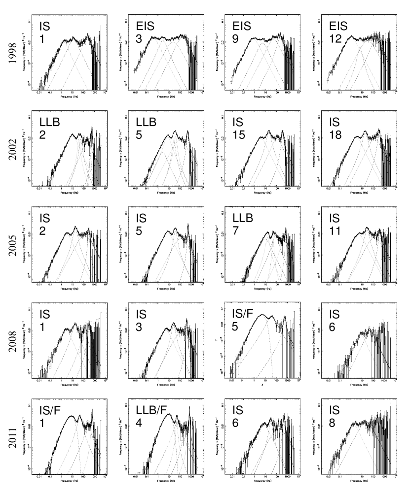
Figure 2.— Selected power spectra of each outburst of SAX J1808. Every row represents a separate outburst as indicated. Each power spectrum has been marked with the number of the interval in its respective outburst and its associated source state (see Table 1 for details). Parameters of the fitted curves are given in Tables 2–5.

Table 2 Characteristic Frequency; $\nu_{\max}$ (Hz)

Interval	$L_{b2}$	$L_{b}$	$L_{h}$	$L_{\text{LF}}$	$L_{{\ell}\text{ow}}$	$L_{\text{hHz}}$	$L_{\ell}$	$L_{u}$
1998 Outburst
1	$\cdots$	$1.83\pm 0.08$	$13.3\pm 0.5$	$\cdots$	$\cdots$	$\cdots$	$\cdots$	$236\pm 14$
2	$\cdots$	$0.408\pm 0.013$	$2.89\pm 0.08$	$\cdots$	$26\pm 2$	$\cdots$	$\cdots$	$155\pm 7$
3	$\cdots$	$0.381\pm 0.018$	$2.79\pm 0.10$	$\cdots$	$24\pm 4$	$\cdots$	$\cdots$	$167\pm 13$
4	$\cdots$	$0.363\pm 0.012$	$2.62\pm 0.07$	$\cdots$	$21.9\pm 1.8$	$\cdots$	$\cdots$	$150\pm 6$
5	$\cdots$	$0.38\pm 0.03$	$2.39\pm 0.16$	$\cdots$	$22\pm 3$	$\cdots$	$\cdots$	$162\pm 20$
6	$\cdots$	$0.347\pm 0.013$	$2.57\pm 0.09$	$\cdots$	$28\pm 3$	$\cdots$	$\cdots$	$177\pm 11$
7	$\cdots$	$0.359\pm 0.014$	$2.63\pm 0.09$	$\cdots$	$21\pm 3$	$\cdots$	$\cdots$	$164\pm 11$
8	$\cdots$	$0.37\pm 0.02$	$2.80\pm 0.17$	$\cdots$	$27\pm 6$	$\cdots$	$\cdots$	$159\pm 16$
9	$\cdots$	$0.81\pm 0.04$	$5.5\pm 0.3$	$\cdots$	$54\pm 8$	$\cdots$	$\cdots$	$213\pm 14$
10	$\cdots$	$1.31\pm 0.07$	$7.6\pm 0.4$	$\cdots$	$52\pm 8$	$\cdots$	$\cdots$	$199\pm 19$
11	$\cdots$	$2.01\pm 0.08$	$13.1\pm 0.8$	$\cdots$	$\cdots$	$\cdots$	$\cdots$	$170\pm 14^{1}$
12	$\cdots$	$1.03\pm 0.03$	$6.5\pm 0.4$	$\cdots$	$32\pm 10$	$\cdots$	$\cdots$	$193\pm 34$
13	$\cdots$	$0.93\pm 0.03$	$\cdots$	$\cdots$	$37\pm 4$	$\cdots$	$\cdots$	$\cdots$
2002 Outburst
1	$\cdots$	$10.4\pm 0.5$	$43.9\pm 2.1$	$\cdots$	$\cdots$	$179\pm 26$	$\cdots$	$567\pm 25$
2	$\cdots$	$9.9\pm 0.2$	$57.8\pm 2.2$	$37.4\pm 1.1$	$\cdots$	$212\pm 34$	$435\pm 12$	$599\pm 5$
3	$7.9\pm 1.5$	$15.4\pm 0.4$	$78.2\pm 2.0$	$47.2\pm 1.8$	$\cdots$	$257\pm 35$	$\cdots$	$698\pm 6$
4	$10.0\pm 1.0$	$15.9\pm 0.2$	$75.7\pm 1.0$	$47.4\pm 0.7$	$\cdots$	$355\pm 43$	$504\pm 3$	$686\pm 5$
5	$2.6\pm 0.5$	$7.6\pm 0.2$	$39.3\pm 1.1$	$28.1\pm 1.1$	$\cdots$	$101\pm 13$	$\cdots$	$497\pm 8$
6	$\cdots$	$3.14\pm 0.05$	$18.01\pm 0.15$	$\cdots$	$\cdots$	$122\pm 9$	$\cdots$	$352\pm 5$
7	$\cdots$	$3.08\pm 0.05$	$18.53\pm 0.19$	$\cdots$	$\cdots$	$122\pm 11$	$\cdots$	$339\pm 5$
8	$\cdots$	$3.00\pm 0.05$	$18.40\pm 0.19$	$\cdots$	$\cdots$	$127\pm 12$	$\cdots$	$332\pm 6$
9	$\cdots$	$2.26\pm 0.05$	$13.6\pm 0.3$	$\cdots$	$\cdots$	$112\pm 12$	$\cdots$	$294\pm 7$
10	$\cdots$	$4.6\pm 0.2$	$24.4\pm 1.0$	$\cdots$	$\cdots$	$98\pm 48$	$\cdots$	$389\pm 21$
11	$\cdots$	$5.00\pm 0.12$	$25.4\pm 0.3$	$\cdots$	$\cdots$	$113\pm 14$	$\cdots$	$393\pm 5$
12	$\cdots$	$4.9\pm 0.2$	$25.1\pm 0.6$	$\cdots$	$\cdots$	$100\pm 25$	$\cdots$	$381\pm 10$
13	$\cdots$	$4.26\pm 0.11$	$23.0\pm 0.3$	$\cdots$	$\cdots$	$120\pm 19$	$\cdots$	$370\pm 7$
14	$\cdots$	$3.41\pm 0.17$	$19.3\pm 0.5$	$\cdots$	$\cdots$	$89\pm 28$	$\cdots$	$332\pm 11$
15	$\cdots$	$3.71\pm 0.10$	$20.2\pm 0.3$	$\cdots$	$\cdots$	$109\pm 10$	$\cdots$	$358\pm 10$
16	$\cdots$	$3.53\pm 0.19$	$23.2\pm 0.7$	$\cdots$	$\cdots$	$88\pm 7$	$\cdots$	$336\pm 17$
17	$\cdots$	$3.41\pm 0.10$	$20.9\pm 0.4$	$\cdots$	$\cdots$	$127\pm 22$	$\cdots$	$326\pm 10$
18	$\cdots$	$3.15\pm 0.07$	$19.2\pm 0.3$	$\cdots$	$\cdots$	$139\pm 27$	$\cdots$	$340\pm 11$
19	$\cdots$	$3.49\pm 0.14$	$20.8\pm 0.5$	$\cdots$	$\cdots$	$187\pm 48$	$\cdots$	$358\pm 14$
20	$\cdots$	$3.73\pm 0.12$	$21.2\pm 0.4$	$\cdots$	$\cdots$	$139\pm 18$	$\cdots$	$332\pm 11$
21	$\cdots$	$3.99\pm 0.15$	$23.1\pm 0.5$	$\cdots$	$\cdots$	$173\pm 51$	$\cdots$	$357\pm 16$
22	$\cdots$	$4.8\pm 0.4$	$28.7\pm 1.0$	$\cdots$	$\cdots$	$\cdots$	$\cdots$	$413\pm 143$
2005 Outburst
1	$\cdots$	$2.6\pm 0.2$	$23.7\pm 1.9$	$\cdots$	$\cdots$	$\cdots$	$\cdots$	$\cdots$
2	$\cdots$	$3.15\pm 0.06$	$18.9\pm 0.2$	$\cdots$	$\cdots$	$122\pm 21$	$\cdots$	$304\pm 10$
3	$\cdots$	$5.51\pm 0.12$	$28.1\pm 0.4$	$\cdots$	$\cdots$	$90\pm 10$	$\cdots$	$399\pm 7$
4	$\cdots$	$7.50\pm 0.14$	$38.5\pm 0.6$	$\cdots$	$\cdots$	$155\pm 35$	$\cdots$	$526\pm 8$
5	$\cdots$	$7.63\pm 0.12$	$38.4\pm 0.6$	$\cdots$	$\cdots$	$121\pm 21$	$\cdots$	$532\pm 5$
6	$\cdots$	$6.67\pm 0.17$	$34.2\pm 0.7$	$\cdots$	$\cdots$	$161\pm 45$	$\cdots$	$494\pm 14$
7	$8.9\pm 1.0$	$15.4\pm 0.3$	$78\pm 4$	$47.9\pm 0.6$	$\cdots$	$438\pm 56^{1}$	$\cdots$	$685\pm 10$
8	$\cdots$	$7.24\pm 0.15$	$36.6\pm 0.5$	$\cdots$	$\cdots$	$136\pm 12$	$\cdots$	$498\pm 11$
9	$3.3\pm 0.7$	$7.9\pm 0.3$	$36.5\pm 0.4$	$\cdots$	$\cdots$	$131\pm 19$	$\cdots$	$488\pm 9$
10	$\cdots$	$6.70\pm 0.16$	$34.4\pm 0.4$	$\cdots$	$\cdots$	$127\pm 27$	$\cdots$	$481\pm 19$
11	$\cdots$	$5.07\pm 0.18$	$28.3\pm 0.6$	$\cdots$	$\cdots$	$138\pm 30$	$\cdots$	$393\pm 25$
2008 Outburst
1	$\cdots$	$2.85\pm 0.10$	$18.7\pm 0.8$	$\cdots$	$\cdots$	$135\pm 17$	$\cdots$	$350\pm 36$
2	$\cdots$	$3.66\pm 0.17$	$19.5\pm 0.4$	$\cdots$	$\cdots$	$118\pm 23$	$\cdots$	$372\pm 14$
3	$\cdots$	$5.35\pm 0.15$	$26.5\pm 0.5$	$\cdots$	$\cdots$	$135\pm 29$	$\cdots$	$415\pm 5$
4	$\cdots$	$9.2\pm 0.5$	$49\pm 2$	$\cdots$	$\cdots$	$\cdots$	$\cdots$	$524\pm 33$
5	$\cdots$	— 2	$37\pm 3$	$\cdots$	$\cdots$	$\cdots$	$\cdots$	$606\pm 44$
6	$\cdots$	$8.7\pm 1.3$	$54\pm 10$	$\cdots$	$\cdots$	$\cdots$	$\cdots$	$\cdots$
7	$\cdots$	$1.72\pm 0.16$	$23\pm 4$	$\cdots$	$\cdots$	$\cdots$	$\cdots$	$\cdots$
2011 Outburst
1	$\cdots$	— 2	$49.1\pm 1.4$	$\cdots$	$\cdots$	$291\pm 203$	$\cdots$	$657\pm 3$
2	$\cdots$	— 2	$38\pm 16$	$\cdots$	$\cdots$	$\cdots$	$\cdots$	$527\pm 226$
3	$\cdots$	— 2	$52\pm 8$	$52.3\pm 0.7$	$\cdots$	$343\pm 22$	$\cdots$	$719\pm 4$
4	$\cdots$	— 2	$59\pm 14$	$51.6\pm 1.5$	$\cdots$	$289\pm 43$	$\cdots$	$712\pm 5$
5	$4.4\pm 1.1$	$15.3\pm 0.8$	$78\pm 4$	$48.8\pm 1.7$	$\cdots$	$\cdots$	$567\pm 9$	$737\pm 10$
6	$\cdots$	$6.8\pm 0.4$	$30.3\pm 1.0$	$\cdots$	$\cdots$	$153\pm 71$	$\cdots$	$478\pm 25$
7	$\cdots$	$3.7\pm 0.3$	$21.1\pm 0.9$	$\cdots$	$\cdots$	$\cdots$	$\cdots$	$245\pm 41$
8	$\cdots$	$1.90\pm 0.13$	$22\pm 3$	$\cdots$	$\cdots$	$\cdots$	$\cdots$	$\cdots$
9	$\cdots$	$0.55\pm 0.04$	$4.6\pm 1.2$	$\cdots$	$\cdots$	$\cdots$	$\cdots$	$113\pm 36$
10	$\cdots$	$0.50\pm 0.04$	$10\pm 7$	$\cdots$	$\cdots$	$\cdots$	$\cdots$	$\cdots$

Table 3 Quality Factor; $Q$

Interval	$L_{b2}$	$L_{b}$	$L_{h}$	$L_{\text{LF}}$	$L_{{\ell}\text{ow}}$	$L_{\text{hHz}}$	$L_{\ell}$	$L_{u}$
1998 Outburst
1	$\cdots$	$0.37\pm 0.04$	$0.29\pm 0.07$	$\cdots$	$\cdots$	$\cdots$	$\cdots$	$0.43\pm 0.10$
2	$\cdots$	$0.21\pm 0.03$	$0.34\pm 0.06$	$\cdots$	$0.11\pm 0.14$	$\cdots$	$\cdots$	$0.35\pm 0.08$
3	$\cdots$	$0.19\pm 0.04$	$0.41\pm 0.08$	$\cdots$	0 ( fixed )	$\cdots$	$\cdots$	$0.24\pm 0.10$
4	$\cdots$	$0.18\pm 0.03$	$0.41\pm 0.06$	$\cdots$	0 ( fixed )	$\cdots$	$\cdots$	$0.38\pm 0.07$
5	$\cdots$	$0.25\pm 0.06$	$0.43\pm 0.12$	$\cdots$	0 ( fixed )	$\cdots$	$\cdots$	$0.32\pm 0.16$
6	$\cdots$	$0.22\pm 0.03$	$0.23\pm 0.06$	$\cdots$	0 ( fixed )	$\cdots$	$\cdots$	$0.30\pm 0.10$
7	$\cdots$	$0.23\pm 0.03$	$0.35\pm 0.08$	$\cdots$	0 ( fixed )	$\cdots$	$\cdots$	$0.21\pm 0.11$
8	$\cdots$	$0.28\pm 0.05$	$0.24\pm 0.12$	$\cdots$	0 ( fixed )	$\cdots$	$\cdots$	$0.41\pm 0.19$
9	$\cdots$	$0.20\pm 0.03$	$0.28\pm 0.13$	$\cdots$	$0.19\pm 0.16$	$\cdots$	$\cdots$	$0.8\pm 0.2$
10	$\cdots$	$0.16\pm 0.03$	$0.5\pm 0.2$	$\cdots$	$0.4\pm 0.2$	$\cdots$	$\cdots$	$0.5\pm 0.2$
11	$\cdots$	$0.12\pm 0.02$	$0.57\pm 0.19$	$\cdots$	$\cdots$	$\cdots$	$\cdots$	0 ( fixed )1
12	$\cdots$	$0.15\pm 0.02$	$1.1\pm 0.5$	$\cdots$	0 ( fixed )	$\cdots$	$\cdots$	$0.4\pm 0.3$
13	$\cdots$	$0.02\pm 0.03$	$\cdots$	$\cdots$	0 ( fixed )	$\cdots$	$\cdots$	$\cdots$
2002 Outburst
1	$\cdots$	$0.35\pm 0.04$	$0.89\pm 0.18$	$\cdots$	$\cdots$	$1.2\pm 0.7$	$\cdots$	0 ( fixed )
2	$\cdots$	$0.35\pm 0.02$	$1.9\pm 0.7$	$2.4\pm 0.6$	$\cdots$	$0.4\pm 0.3$	$12\pm 113$	$7.7\pm 1.7$
3	$0.35\pm 0.06$	$1.3\pm 0.3$	$2.8\pm 0.8$	$2.0\pm 0.5$	$\cdots$	$0.6\pm 0.3$	$\cdots$	$8.2\pm 1.9$
4	$0.28\pm 0.02$	$1.3\pm 0.2$	$3.4\pm 0.6$	$2.3\pm 0.3$	$\cdots$	0 ( fixed )	27 ( fixed )	$7.0\pm 1.2$
5	$0.36\pm 0.07$	$0.58\pm 0.10$	$1.9\pm 0.4$	$1.9\pm 0.3$	$\cdots$	0 ( fixed )	$\cdots$	$3.0\pm 0.3$
6	$\cdots$	$0.236\pm 0.012$	$0.85\pm 0.04$	$\cdots$	$\cdots$	$0.19\pm 0.08$	$\cdots$	$2.3\pm 0.3$
7	$\cdots$	$0.260\pm 0.014$	$0.83\pm 0.04$	$\cdots$	$\cdots$	$0.20\pm 0.11$	$\cdots$	$2.3\pm 0.4$
8	$\cdots$	$0.279\pm 0.013$	$0.86\pm 0.05$	$\cdots$	$\cdots$	$0.24\pm 0.12$	$\cdots$	$2.4\pm 0.5$
9	$\cdots$	$0.217\pm 0.016$	$0.65\pm 0.06$	$\cdots$	$\cdots$	$0.14\pm 0.11$	$\cdots$	$1.9\pm 0.5$
10	$\cdots$	$0.33\pm 0.04$	$1.1\pm 0.3$	$\cdots$	$\cdots$	0 ( fixed )	$\cdots$	$2.8\pm 1.8$
11	$\cdots$	$0.267\pm 0.018$	$1.18\pm 0.10$	$\cdots$	$\cdots$	$0.15\pm 0.19$	$\cdots$	$4.4\pm 0.6$
12	$\cdots$	$0.30\pm 0.03$	$1.14\pm 0.17$	$\cdots$	$\cdots$	0 ( fixed )	$\cdots$	$5\pm 3$
13	$\cdots$	$0.265\pm 0.019$	$0.93\pm 0.07$	$\cdots$	$\cdots$	$0.3\pm 0.2$	$\cdots$	$2.8\pm 0.8$
14	$\cdots$	$0.27\pm 0.04$	$0.98\pm 0.16$	$\cdots$	$\cdots$	0 ( fixed )	$\cdots$	$4\pm 2$
15	$\cdots$	$0.240\pm 0.018$	$0.99\pm 0.08$	$\cdots$	$\cdots$	$0.32\pm 0.16$	$\cdots$	$2.5\pm 0.5$
16	$\cdots$	$0.26\pm 0.04$	$0.72\pm 0.10$	$\cdots$	$\cdots$	$1.4\pm 0.6$	$\cdots$	$1.5\pm 0.4$
17	$\cdots$	$0.255\pm 0.021$	$0.88\pm 0.09$	$\cdots$	$\cdots$	$0.3\pm 0.2$	$\cdots$	$2.6\pm 0.9$
18	$\cdots$	$0.245\pm 0.017$	$0.91\pm 0.07$	$\cdots$	$\cdots$	$0.18\pm 0.16$	$\cdots$	$2.0\pm 0.7$
19	$\cdots$	$0.25\pm 0.03$	$0.85\pm 0.10$	$\cdots$	$\cdots$	0 ( fixed )	$\cdots$	$3.7\pm 1.9$
20	$\cdots$	$0.24\pm 0.02$	$1.01\pm 0.09$	$\cdots$	$\cdots$	$0.34\pm 0.19$	$\cdots$	$3.0\pm 1.3$
21	$\cdots$	$0.24\pm 0.03$	$1.04\pm 0.11$	$\cdots$	$\cdots$	0 ( fixed )	$\cdots$	$3.2\pm 1.6$
22	$\cdots$	$0.21\pm 0.06$	$1.4\pm 0.2$	$\cdots$	$\cdots$	$\cdots$	$\cdots$	0 ( fixed )
2005 Outburst
1	$\cdots$	$0.49\pm 0.12$	$0.7\pm 0.2$	$\cdots$	$\cdots$	$\cdots$	$\cdots$	$\cdots$
2	$\cdots$	$0.315\pm 0.017$	$1.08\pm 0.07$	$\cdots$	$\cdots$	0 ( fixed )	$\cdots$	$3.4\pm 1.7$
3	$\cdots$	$0.324\pm 0.019$	$1.28\pm 0.10$	$\cdots$	$\cdots$	$0.40\pm 0.16$	$\cdots$	$4.5\pm 0.9$
4	$\cdots$	$0.308\pm 0.016$	$1.31\pm 0.11$	$\cdots$	$\cdots$	0 ( fixed )	$\cdots$	$4.4\pm 1.5$
5	$\cdots$	$0.319\pm 0.014$	$1.37\pm 0.12$	$\cdots$	$\cdots$	0 ( fixed )	$\cdots$	$5.8\pm 1.9$
6	$\cdots$	$0.41\pm 0.03$	$1.6\pm 0.2$	$\cdots$	$\cdots$	0 ( fixed )	$\cdots$	$9\pm 6$
7	$0.26\pm 0.02$	$1.3\pm 0.2$	$0.73\pm 0.15$	$4.0\pm 1.0$	$\cdots$	$0.8\pm 0.5^{1}$	$\cdots$	$7\pm 6$
8	$\cdots$	$0.293\pm 0.018$	$1.63\pm 0.12$	$\cdots$	$\cdots$	$0.53\pm 0.18$	$\cdots$	$3.8\pm 1.0$
9	$0.34\pm 0.04$	$0.69\pm 0.11$	$1.30\pm 0.08$	$\cdots$	$\cdots$	$0.24\pm 0.15$	$\cdots$	$2.7\pm 0.5$
10	$\cdots$	$0.253\pm 0.019$	$1.56\pm 0.12$	$\cdots$	$\cdots$	$0.3\pm 0.3$	$\cdots$	$2.3\pm 0.9$
11	$\cdots$	$0.18\pm 0.02$	$0.95\pm 0.11$	$\cdots$	$\cdots$	0 ( fixed )	$\cdots$	$2.1\pm 0.8$
2008 Outburst
1	$\cdots$	$0.35\pm 0.04$	$0.79\pm 0.09$	$\cdots$	$\cdots$	$1.0\pm 0.4$	$\cdots$	$2.4\pm 1.0$
2	$\cdots$	$0.20\pm 0.04$	$1.45\pm 0.18$	$\cdots$	$\cdots$	0 ( fixed )	$\cdots$	$4\pm 4$
3	$\cdots$	$0.28\pm 0.02$	$1.20\pm 0.11$	$\cdots$	$\cdots$	0 ( fixed )	$\cdots$	$6\pm 4$
4	$\cdots$	$0.29\pm 0.03$	$0.67\pm 0.13$	$\cdots$	$\cdots$	$\cdots$	$\cdots$	$1.5\pm 0.5$
5	$\cdots$	—2	$0.46\pm 0.05$	$\cdots$	$\cdots$	$\cdots$	$\cdots$	$2.2\pm 0.7$
6	$\cdots$	$0.35\pm 0.17$	$0.3\pm 0.5$	$\cdots$	$\cdots$	$\cdots$	$\cdots$	$\cdots$
7	$\cdots$	0 ( fixed )	0 ( fixed )	$\cdots$	$\cdots$	$\cdots$	$\cdots$	$\cdots$
2011 Outburst
1	$\cdots$	—2	$1.09\pm 0.08$	$\cdots$	$\cdots$	$0.5\pm 0.5$	$\cdots$	$9\pm 3$
2	$\cdots$	—2	$0.4\pm 0.3$	$\cdots$	$\cdots$	$\cdots$	$\cdots$	$0.9\pm 0.9$
3	$\cdots$	—2	$0.42\pm 0.10$	$5\pm 3$	$\cdots$	$3.3\pm 1.3$	$\cdots$	$7.6\pm 1.0$
4	$\cdots$	—2	$0.60\pm 0.18$	$3.3\pm 1.3$	$\cdots$	$1.6\pm 0.8$	$\cdots$	$7.8\pm 1.2$
5	$0.50\pm 0.13$	$0.54\pm 0.12$	$1.9\pm 0.9$	$4\pm 4$	$\cdots$	$\cdots$	14 ( fixed )	$10\pm 5$
6	$\cdots$	$0.23\pm 0.04$	$1.5\pm 0.3$	$\cdots$	$\cdots$	0 ( fixed )	$\cdots$	$3\pm 2$
7	$\cdots$	$0.27\pm 0.05$	$1.0\pm 0.2$	$\cdots$	$\cdots$	$\cdots$	$\cdots$	$0.4\pm 0.2$
8	$\cdots$	$0.27\pm 0.05$	0 ( fixed )	$\cdots$	$\cdots$	$\cdots$	$\cdots$	$\cdots$
9	$\cdots$	$0.20\pm 0.05$	0 ( fixed )	$\cdots$	$\cdots$	$\cdots$	$\cdots$	0 ( fixed )
10	$\cdots$	0 ( fixed )	0 ( fixed )	$\cdots$	$\cdots$	$\cdots$	$\cdots$	$\cdots$

Table 4 RMS Amplitudes; $r$ (%)

Interval	$L_{b2}$	$L_{b}$	$L_{h}$	$L_{\text{LF}}$	$L_{{\ell}\text{ow}}$	$L_{\text{hHz}}$	$L_{\ell}$	$L_{u}$
1998 Outburst
1	$\cdots$	$14.4\pm 0.5$	$17.8\pm 0.7$	$\cdots$	$\cdots$	$\cdots$	$\cdots$	$18.6\pm 0.7$
2	$\cdots$	$19.0\pm 0.3$	$16.6\pm 0.8$	$\cdots$	$16.8\pm 1.6$	$\cdots$	$\cdots$	$20.1\pm 1.1$
3	$\cdots$	$19.9\pm 0.4$	$15.7\pm 0.9$	$\cdots$	$17.7\pm 0.9$	$\cdots$	$\cdots$	$20.9\pm 1.2$
4	$\cdots$	$20.5\pm 0.3$	$15.5\pm 0.6$	$\cdots$	$18.9\pm 0.4$	$\cdots$	$\cdots$	$20.0\pm 0.7$
5	$\cdots$	$20.2\pm 0.7$	$15.4\pm 1.3$	$\cdots$	$19.0\pm 1.0$	$\cdots$	$\cdots$	$19.2\pm 1.5$
6	$\cdots$	$19.6\pm 0.4$	$17.5\pm 0.7$	$\cdots$	$19.1\pm 0.6$	$\cdots$	$\cdots$	$19.1\pm 1.0$
7	$\cdots$	$20.5\pm 0.4$	$15.7\pm 0.9$	$\cdots$	$18.3\pm 0.7$	$\cdots$	$\cdots$	$21.0\pm 1.1$
8	$\cdots$	$19.3\pm 0.7$	$17.0\pm 1.3$	$\cdots$	$19.1\pm 1.2$	$\cdots$	$\cdots$	$19.0\pm 1.9$
9	$\cdots$	$19.1\pm 0.5$	$14.6\pm 1.5$	$\cdots$	$19\pm 2$	$\cdots$	$\cdots$	$16\pm 2$
10	$\cdots$	$18.6\pm 0.6$	$11.8\pm 1.7$	$\cdots$	$15\pm 3$	$\cdots$	$\cdots$	$18\pm 2$
11	$\cdots$	$18.6\pm 0.4$	$10.7\pm 1.1$	$\cdots$	$\cdots$	$\cdots$	$\cdots$	$24.2\pm 0.5^{1}$
12	$\cdots$	$21.5\pm 0.2$	$8.2\pm 1.6$	$\cdots$	$19.0\pm 1.8$	$\cdots$	$\cdots$	$18\pm 3$
13	$\cdots$	$25.4\pm 0.3$	$\cdots$	$\cdots$	$28.3\pm 0.8$	$\cdots$	$\cdots$	$\cdots$
2002 Outburst
1	$\cdots$	$17.7\pm 0.5$	$13.7\pm 1.0$	$\cdots$	$\cdots$	$8.4\pm 1.7$	$\cdots$	$8.0\pm 1.2$
2	$\cdots$	$17.4\pm 0.2$	$8.2\pm 1.6$	$7.3\pm 1.0$	$\cdots$	$11.8\pm 1.6$	$4.0\pm 1.0$	$8.7\pm 0.6$
3	$9.6\pm 1.3$	$9.8\pm 1.3$	$7.1\pm 1.1$	$7.3\pm 0.9$	$\cdots$	$9.9\pm 1.1$	$\cdots$	$8.3\pm 0.7$
4	$12.2\pm 1.0$	$9.0\pm 1.1$	$6.0\pm 0.5$	$7.2\pm 0.4$	$\cdots$	$12.8\pm 0.4$	$2.5\pm 0.4$	$7.6\pm 0.6$
5	$6.8\pm 1.7$	$14.2\pm 1.0$	$9.3\pm 1.4$	$7.8\pm 1.3$	$\cdots$	$15.5\pm 0.5$	$\cdots$	$9.7\pm 0.4$
6	$\cdots$	$15.36\pm 0.12$	$15.3\pm 0.3$	$\cdots$	$\cdots$	$15.7\pm 0.7$	$\cdots$	$10.1\pm 0.7$
7	$\cdots$	$15.05\pm 0.13$	$15.3\pm 0.4$	$\cdots$	$\cdots$	$15.1\pm 0.9$	$\cdots$	$10.6\pm 0.8$
8	$\cdots$	$15.17\pm 0.12$	$15.6\pm 0.4$	$\cdots$	$\cdots$	$15.0\pm 0.9$	$\cdots$	$10.0\pm 0.9$
9	$\cdots$	$16.08\pm 0.18$	$14.0\pm 0.6$	$\cdots$	$\cdots$	$17.4\pm 1.1$	$\cdots$	$10.4\pm 1.3$
10	$\cdots$	$15.24\pm 0.4$	$14.1\pm 1.7$	$\cdots$	$\cdots$	$15.6\pm 1.3$	$\cdots$	$10\pm 2$
11	$\cdots$	$15.7\pm 0.2$	$14.0\pm 0.7$	$\cdots$	$\cdots$	$14.7\pm 1.2$	$\cdots$	$9.8\pm 0.6$
12	$\cdots$	$15.4\pm 0.3$	$13.7\pm 1.0$	$\cdots$	$\cdots$	$15.9\pm 0.8$	$\cdots$	$8.9\pm 1.1$
13	$\cdots$	$15.2\pm 0.2$	$15.9\pm 0.6$	$\cdots$	$\cdots$	$14.0\pm 1.7$	$\cdots$	$10.8\pm 1.2$
14	$\cdots$	$14.7\pm 0.3$	$14.5\pm 1.1$	$\cdots$	$\cdots$	$15.7\pm 0.9$	$\cdots$	$9.2\pm 1.4$
15	$\cdots$	$15.44\pm 0.19$	$15.1\pm 0.6$	$\cdots$	$\cdots$	$14.8\pm 1.1$	$\cdots$	$10.3\pm 0.9$
16	$\cdots$	$15.0\pm 0.4$	$17.5\pm 0.7$	$\cdots$	$\cdots$	$9.1\pm 1.5$	$\cdots$	$14.2\pm 1.2$
17	$\cdots$	$15.4\pm 0.2$	$15.7\pm 0.7$	$\cdots$	$\cdots$	$14.5\pm 1.5$	$\cdots$	$9.8\pm 1.4$
18	$\cdots$	$16.15\pm 0.18$	$15.3\pm 0.5$	$\cdots$	$\cdots$	$15.8\pm 1.6$	$\cdots$	$11.0\pm 1.8$
19	$\cdots$	$15.7\pm 0.3$	$15.3\pm 0.6$	$\cdots$	$\cdots$	$17.1\pm 1.3$	$\cdots$	$8.9\pm 1.6$
20	$\cdots$	$15.6\pm 0.2$	$15.6\pm 0.6$	$\cdots$	$\cdots$	$15.2\pm 1.4$	$\cdots$	$9.2\pm 1.5$
21	$\cdots$	$15.9\pm 0.3$	$15.0\pm 0.7$	$\cdots$	$\cdots$	$17.2\pm 1.3$	$\cdots$	$8.8\pm 1.9$
22	$\cdots$	$15.7\pm 0.5$	$14.3\pm 0.9$	$\cdots$	$\cdots$	$\cdots$	$\cdots$	$21\pm 2$
2005 Outburst
1	$\cdots$	$13.5\pm 0.8$	$18.4\pm 1.3$	$\cdots$	$\cdots$	$\cdots$	$\cdots$	$\cdots$
2	$\cdots$	$15.28\pm 0.14$	$14.5\pm 0.4$	$\cdots$	$\cdots$	$16.2\pm 0.7$	$\cdots$	$7.4\pm 1.3$
3	$\cdots$	$14.72\pm 0.18$	$13.0\pm 0.6$	$\cdots$	$\cdots$	$12.4\pm 1.0$	$\cdots$	$8.7\pm 0.7$
4	$\cdots$	$16.47\pm 0.16$	$11.9\pm 0.5$	$\cdots$	$\cdots$	$13.1\pm 0.6$	$\cdots$	$8.5\pm 0.8$
5	$\cdots$	$16.72\pm 0.15$	$11.6\pm 0.6$	$\cdots$	$\cdots$	$13.8\pm 0.6$	$\cdots$	$8.8\pm 0.5$
6	$\cdots$	$16.6\pm 0.2$	$12.1\pm 0.7$	$\cdots$	$\cdots$	$14.3\pm 0.9$	$\cdots$	$5.9\pm 1.1$
7	$12.1\pm 0.9$	$8.4\pm 1.2$	$11.6\pm 0.9$	$5.0\pm 0.7$	$\cdots$	$9.2\pm 1.4^{1}$	$\cdots$	$6.2\pm 0.9$
8	$\cdots$	$17.19\pm 0.17$	$12.9\pm 0.5$	$\cdots$	$\cdots$	$13.2\pm 1.0$	$\cdots$	$9.5\pm 1.0$
9	$8.7\pm 1.9$	$13.2\pm 1.3$	$14.1\pm 0.5$	$\cdots$	$\cdots$	$12.8\pm 1.0$	$\cdots$	$10.6\pm 0.8$
10	$\cdots$	$15.8\pm 0.2$	$13.1\pm 0.6$	$\cdots$	$\cdots$	$11.9\pm 1.6$	$\cdots$	$9.6\pm 1.4$
11	$\cdots$	$15.9\pm 0.2$	$14.1\pm 0.8$	$\cdots$	$\cdots$	$14.8\pm 0.7$	$\cdots$	$8.6\pm 1.0$
2008 Outburst
1	$\cdots$	$15.0\pm 0.2$	$16.4\pm 0.5$	$\cdots$	$\cdots$	$11.8\pm 1.2$	$\cdots$	$10.4\pm 1.7$
2	$\cdots$	$15.5\pm 0.3$	$13.0\pm 0.7$	$\cdots$	$\cdots$	$19.1\pm 0.9$	$\cdots$	$9.1\pm 1.6$
3	$\cdots$	$15.4\pm 0.2$	$13.6\pm 0.5$	$\cdots$	$\cdots$	$15.8\pm 0.7$	$\cdots$	$9.1\pm 0.8$
4	$\cdots$	$15.3\pm 0.5$	$14.2\pm 0.8$	$\cdots$	$\cdots$	$\cdots$	$\cdots$	$12.3\pm 1.2$
5	$\cdots$	—2	$29.2\pm 1.0$	$\cdots$	$\cdots$	$\cdots$	$\cdots$	$14.1\pm 1.6$
6	$\cdots$	$11\pm 2$	$14\pm 3$	$\cdots$	$\cdots$	$\cdots$	$\cdots$	$\cdots$
7	$\cdots$	$17.9\pm 0.8$	$23.5\pm 1.1$	$\cdots$	$\cdots$	$\cdots$	$\cdots$	$\cdots$
2011 Outburst
1	$\cdots$	—2	$20.2\pm 0.9$	$\cdots$	$\cdots$	$17\pm 8$	$\cdots$	$11.5\pm 0.8$
2	$\cdots$	—2	$14\pm 3$	$\cdots$	$\cdots$	$\cdots$	$\cdots$	$13\pm 4$
3	$\cdots$	—2	$23.7\pm 1.2$	$7.2\pm 1.4$	$\cdots$	$7.3\pm 1.1$	$\cdots$	$13.4\pm 0.6$
4	$\cdots$	—2	$18.5\pm 1.7$	$9\pm 3$	$\cdots$	$9.2\pm 1.9$	$\cdots$	$13.4\pm 0.7$
5	$6.8\pm 1.8$	$14.3\pm 1.1$	$7.8\pm 1.4$	$5.3\pm 1.2$	$\cdots$	$\cdots$	$4.1\pm 0.8$	$7.1\pm 0.9$
6	$\cdots$	$17.0\pm 0.5$	$12.3\pm 1.2$	$\cdots$	$\cdots$	$15.9\pm 1.7$	$\cdots$	$11\pm 2$
7	$\cdots$	$16.5\pm 0.6$	$15.4\pm 1.2$	$\cdots$	$\cdots$	$\cdots$	$\cdots$	$21.2\pm 1.8$
8	$\cdots$	$16.4\pm 0.6$	$21.4\pm 0.7$	$\cdots$	$\cdots$	$\cdots$	$\cdots$	$\cdots$
9	$\cdots$	$22.0\pm 0.8$	$18.7\pm 1.2$	$\cdots$	$\cdots$	$\cdots$	$\cdots$	$28\pm 3$
10	$\cdots$	$33.8\pm 1.1$	$29\pm 4$	$\cdots$	$\cdots$	$\cdots$	$\cdots$	$\cdots$

Table 5 Schechter function fit parameters.

Interval	$\alpha$	$\nu_{\text{cut}}$	r
		(Hz)	(%)
2008
5	$-0.52\pm 0.02$	$3.33\pm 0.10$	$28.4\pm 0.3$
2011
1	$-0.450\pm 0.013$	$5.63\pm 0.09$	$25.48\pm 0.10$
2	$-0.79\pm 0.15$	$5.6\pm 1.0$	$15.4\pm 1.3$
3	$-0.59\pm 0.02$	$4.95\pm 0.17$	$26.75\pm 0.15$
4	$-0.60\pm 0.02$	$5.67\pm 0.16$	$27.1\pm 0.3$

4.1. 1998

The first RXTE detection of SAX J1808 was with a scan observation on MJD 50915 (day 9 of Figure 1, Marshall et al., 1998), during which the source flux was $59$ mCrab. At this time the source was in the island state showing a power spectrum that can be fitted with three Lorentzians ($L_{b}$, $L_{h}$ and $L_{u}$).

The first pointed RXTE observation was five days later on MJD 50920, at which time the flux had decayed to $\sim$43 mCrab. The soft color was decreasing, while the hard color increased. The power spectrum shifted to lower frequencies and requires an additional $L_{{\ell}\text{ow}}$ component, clearly showing that SAX J1808 transitioned to the extreme island state.

Over the following 14 days the flux and soft colors steadily decreased, while the hard color remained constant for 5 days before also starting to decay. The flux and soft color evolution transitioned into a faster decay on MJD 50929 (day 23). The flux decay briefly slowed down three days later. Finally the flux dropped below the detection limit on MJD 50934 (day 28), as the source returned to quiescence. During the entire decay SAX J1808 remained in the extreme island state.

4.2. 2002

In the 2002 outburst SAX J1808 was first detected with RXTE on MJD 52560. When pointed RXTE observations commenced on MJD 52562 (day 6) the source was already close to the flux maximum. In interval 1 the power spectrum clearly reflects the island state, showing $L_{b}$, $L_{h}$, $L_{\text{hHz}}$ and $L_{u}$. In interval 2 both colors decrease as SAX J1808 appears to be transitioning to the lower-left banana. The power spectrum now shows a complex morphology, requiring at least six Lorentzian components. At $\sim$50 Hz the $L_{\text{LF}}$ component appears, and we detect a $2.8\sigma$ feature at $\nu_{0}=434\pm 12$ Hz which we tentatively accept as the lower kHz QPO, $L_{\ell}$, as the upper kHz QPO is seen simultaneously at $\nu_{0,u}=597.9\pm 5.3$ Hz.

In the following observations a flux maximum of $\sim$85 mCrab is reached, and maintained for about a day. The lower kHz QPO is detected at higher significance with $\nu_{0,\ell}=503.5\pm 3.1$ Hz and $\nu_{0,u}=684.5\pm 4.9$ Hz, and a second noise component appears near $L_{b}$, providing further evidence that the source indeed transitioned to the lower-left banana.

As the flux starts to decay on MJD 52564 (day 8), both colors increase and SAX J1808 transitions back into the island state. From interval 7 (day 9) the soft color starts to decrease once more, while the hard color remains roughly constant. The power spectrum shows very little change and remains consistent with an island state morphology.

After reaching a flux minimum on MJD 52579 (day 23), SAX J1808 entered the prolonged outburst tail (Patruno et al., 2009), which continued for 24 days.

4.3. 2005

Routine monitoring with RXTE revealed a new outburst of SAX J1808 on MJD 53521 (day 1) (Markwardt et al., 2005). In the following days the flux steadily increased until a maximum of $\sim$60 mCrab was reached approximately five days after first detection.

While the flux increased to its maximum (intervals 1–6) the hard color showed a steady decay, whereas the soft color remained roughly constant. During this time the power spectrum is that of the island state, showing $L_{b}$, $L_{h}$, $L_{\text{hHz}}$ and $L_{u}$.

The flux maximum of 60 mCrab is reached on MJD 53528 (day 6, interval 7). In this interval both colors drop sufficiently to suggest a transition to the lower-left banana. The power spectrum confirms this transition with the appearance of $L_{b2}$ and a narrow QPO at 58 Hz, which we identify as $L_{\text{LF}}$. Additionally a broad feature appears at $\nu_{\max}=428$ Hz, which is difficult to identify as the low $Q$ suggests it is $L_{\text{hHz}}$, while the frequency suggests it is $L_{\ell}$. The amplitude of 9% rms lies roughly in between $L_{\text{hHz}}$ and $L_{\ell}$. We label it as $L_{\text{hHz}}$, noting that it is not a ‘clean’ detection.

After reaching the flux maximum, both colors increased as SAX J1808 transitioned to the island state. Over the following seven days the flux and soft color decayed, while the hard color increased. On MJD 53542 (day 20) SAX J1808 was only marginally detected, marking the end of the main outburst and the start of a 40 day prolonged outburst tail (Patruno et al., 2009).

4.4. 2008

On MJD 54731 (day 1) SAX J1808 was again detected in outburst with RXTE. As in 2005 the rise to maximum flux was well sampled, and showed the same behavior: as the flux increased, the hard color decreased and the soft color remained constant. The power spectrum is an island state one and is well described with four Lorentzians ($L_{b}$, $L_{h}$, $L_{\text{hHz}}$ and $L_{u}$.)

During its luminosity maximum (intervals 3–4, days 3–7) SAX J1808 reached a flux of $55$ mCrab, the lowest flux maximum of all outbursts. The soft and hard colors again show a drop prior to the onset of the flux decay. Although this drop is as deep as seen in the other outbursts, the power spectrum indicates the source does not make a state transition to the lower-left banana. A sharp feature does appear at $\nu=283$ Hz. Given $\nu_{u}=520$ Hz this is roughly where $L_{\ell}$ is expected to appear, but at 2$\sigma$ it is not significant.

On MJD 54737 (day 6) both colors increase as the flux starts to decay. At this point (interval 5) the power spectrum shows an unexpected deviation from the regular island state morphology as the high luminosity flaring now dominates the power spectrum below 10 Hz (Bult & van der Klis, 2014). With a fractional rms amplitude of $\sim$30%, the flaring overwhelms the $L_{b}$ component that is normally seen in the same frequency range. We therefore cannot fit the $L_{b}$ component to the data. The flaring remains present for about three days, after which the power spectrum returns to the regular island state shape.

On MJD 54748 (day 19) SAX J1808 enters the prolonged outburst tail, which lasts for 30 days.

4.5. 2011

The first pointed RXTE observation of SAX J1808’s seventh outburst was on MJD 55869 (day 2), roughly five days after the initial detection with SWIFT (Markwardt et al., 2011). The low frequency region of the power spectrum was again dominated by high luminosity flaring. In the first two intervals the mid/high frequency domain required three Lorentzians ($L_{h}$, $L_{\text{hHz}}$ and $L_{u}$), which suggests that despite the low color values the source was still in the island state.

On MJD 55871 (day 4, interval 3), a maximum flux of 80 mCrab was reached, which correlated with a drop in amplitude of the flaring component. In the next interval the amplitude of the flaring increased again and the high frequency components suggested the source transitioned to the lower-left banana. The feature which is normally identified as the hump component has a central peak, but also broad wings and hence is not well described by a single Lorentzian profile, but instead requires two Lorentzians for a satisfactory fit: one to describe the sharp QPO and one for the overlapping noise component. We identify the broader noise component as $L_{h}$ and the peaked QPO as $L_{\text{LF}}$, but note that this identification is uncertain as the two components are not well resolved, and may be distorted by the high frequency wing of the high luminosity flaring component.

In interval 5 (day 7) the high luminosity flaring disappears, while colors remain at low values. The $L_{\text{LF}}$ component is now clearly present in the power spectrum and the marginal detection ($2.8\sigma$) of the lower kHz QPO at $\nu_{0,\ell}=566.6\pm 9.4$ Hz with a simultaneous $\nu_{0,u}=736.1\pm 9.7$ Hz confirms SAX J1808 entered the lower-left banana.

In interval 6 (day 8) the colors increased as the source switched back to the island state. The power spectrum can be described with $L_{b}$, $L_{h}$, $L_{\text{hHz}}$ and $L_{u}$. In the following ten days SAX J1808 showed a regular decay with the soft color decreasing with flux while the hard color increased. During this time the power spectral components smoothly move to lower frequencies, before transitioning into the extreme island state in the last two intervals.

4.6. The 410 Hz QPO

In the outburst of 2002, between MJD 52565 and MJD 52573, Wijnands et al. (2003) detected a sharp QPO at $\sim$410 Hz with an amplitude of $\sim$2.5% rms in the 3–60 keV energy range. We search all outbursts for this 410 Hz QPO using our 2–20 keV band, which gives a better signal to noise ratio. Due to the small amplitude of the QPO, we nearly always have to average multiple intervals to obtain a significant detection.

We detect the 410 Hz QPO at $>3\sigma$ significance in the outbursts of 2002, 2005 and 2008 (see Table 6), but not in the outbursts of 1998 and 2011, for which we obtain 95% confidence upper limits for the amplitude of $\sim$3%. The QPO amplitude varies between 2.1% and 3.6%, and shows no relation with $\nu_{410}$ or $\nu_{u}$. The characteristic frequency varies smoothly between $409.6$ and $416.6$ Hz and is correlated with the upper kHz QPO frequency.

Table 6 410 Hz QPO Fit Parameters

Intervals	$\nu_{410}$	Q	r	P/$\sigma_{P}$	$\nu_{b}$	$\nu_{h}$	$\nu_{u}$
	(Hz)		(%)		(Hz)	(Hz)	(Hz)
2002
6, 7, 8	$409.6\pm 0.6$	$80^{+29}_{-21}$	$2.1\pm 0.3$	4.4	$3.07\pm 0.04$	$18.30\pm 0.10$	$330\pm 3$
10, 11	$414.7\pm 0.6$	$70^{+28}_{-17}$	$3.6\pm 0.5$	4.3	$4.95\pm 0.11$	$25.3\pm 0.3$	$383\pm 6$
12, 13, 15	$410.8\pm 1.1$	$41^{+17}_{-12}$	$3.4\pm 0.5$	3.6	$4.02\pm 0.07$	$22.1\pm 0.2$	$349\pm 7$
2005
3	$416.6\pm 0.8$	$98^{+49}_{-21}$	$3.2\pm 0.5$	4.1	$5.51\pm 0.09$	$28.2\pm 0.3$	$390\pm 7$
2008
1, 2, 3	$416.5\pm 0.9$	$92^{+92}_{-38}$	$2.7\pm 0.5$	3.4	$4.55\pm 0.08$	$22.8\pm 0.4$	$399\pm 10$

Note. — Fit parameters for the 410 Hz feature, its significance ($P/\sigma_{P}$), and the simultaneously measured $\nu_{\max}$ of break and hump components and the upper kHz QPO.

We find the 410 Hz QPO is present in all observations in which $L_{u}$ has $320\leq\nu_{0}\leq 401$ Hz and the flux is higher than 40 mCrab (Figure 3). An exception is interval 14 of the 2002 outburst (grey point in Figure 3 zoom-in), for which we find a 95% confidence upper limit on $r_{410}$ of 3.4%; comparable to the typical amplitude. Due to their lower count rates, the observations below 40 mCrab have higher upper limits on the amplitude ($\sim$4%) and are therefore also consistent with the QPO being below the detection threshold (also see section 5.1.5).

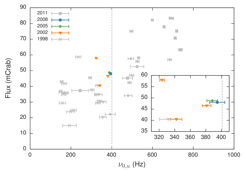
Figure 3.— Overview of the 410 Hz QPO detections. We show flux vs. the upper kHz QPO centroid frequency for all intervals in grey. Intervals in which the 410 Hz QPO was detected are marked in yellow (2002), green (2005), and blue (2008). The vertical dashed line marks the spin frequency ($\nu_{\text{spin}}=401$ Hz). The inset shows a zoom-in of the detection region.

The 410 Hz QPO is only seen in the island state, but is not related to a specific stage of the outburst evolution. In 2005 the QPO was detected during the rise to outburst, in 2008 at the maximum luminosity, while in 2002 the QPO was seen during the flux decay.

The proximity to the 401 Hz spin frequency suggests $L_{410}$ may be an upper sideband of the pulsations. If this is the case then a similar feature might be present at the lower sideband frequency of $\sim$392 Hz. Using the same data selection for which we detected $L_{410}$, we searched for the lower sideband, but no significant features were found, giving a 95% confidence upper limit on the fractional rms of 1.1% to 2.3%. To improve sensitivity we use the shift-and-add method (Méndez et al., 1998) in which we shift the power spectra before averaging them, such that the frequency of the predicted lower sideband feature, $2\nu_{\text{spin}}-\nu_{410}$, is expected at 390 Hz. Again, a lower sideband is not observed.

5. Discussion

It is common practice to study the variability properties of X-ray binaries by considering the relation between the frequencies of several components of the power spectrum. This approach is based on the success of the WK (Wijnands & van der Klis, 1999) and PBK (Psaltis et al., 1999) relations, which show frequency correlations over several orders of magnitude, linking the variability components of neutron star and black hole binaries.

Applied to atoll sources the WK relation considers the correlation between the break frequency versus the $L_{\text{LF}}$ or $L_{h}$ frequency, whereas the PBK relation considers the correlation between the low frequency QPOs and the second highest frequency feature in the power spectrum. For the higher luminosity lower-left banana state this would be $L_{\ell}$, while for the lower luminosity extreme island state it is $L_{{\ell}\text{ow}}$. In the island state it is unclear which component should be considered as neither $L_{{\ell}\text{ow}}$ or $L_{\ell}$ are observed (also see section 5.1.2).

For atoll sources van Straaten et al. (2003) suggested a scheme of correlations for the frequencies of several Lorentzian components plotted against the frequency of $L_{u}$. This scheme of correlations encompasses the WK and PBK relations and is the same across different atoll sources. AMXPs also follow this atoll correlation scheme, although they tend to be shifted in their $\nu_{u}$ by a constant factor of 1.1–1.6, which differs per source (van Straaten et al., 2005; Linares et al., 2005).

A complication in considering frequency relations comes from the fact that the characteristic frequency of the Lorentzian function may not be the physical frequency of the variability mechanism. In this work we used $\nu_{\max}$ as the characteristic frequency, which allows to treat QPO and noise components on the same footing, and tends to reduce the scatter on frequency correlations (Belloni et al., 2002). However, models involving resonances or beat frequencies tend to be defined in terms of the centroid frequency $\nu_{0}=\nu_{\max}/\sqrt{1+1/(4Q^{2})}$. For narrow QPOs (high Q) these two frequencies are almost the same, while for broad noise components (low Q) $\nu_{0}$ is significantly smaller than $\nu_{\rm max}$. We will continue to consider the frequency relations in terms of $\nu_{\max}$ unless explicitly stated otherwise.

Further difficulty in interpreting frequency relations comes from ambiguities in the identification of the variability components. In particular when measurements deviate from a correlation, it could either indicate a break down of the relation, or a mislabeling of the considered component. It is therefore useful to distinguish between secure and more uncertain identification of the power spectral components.

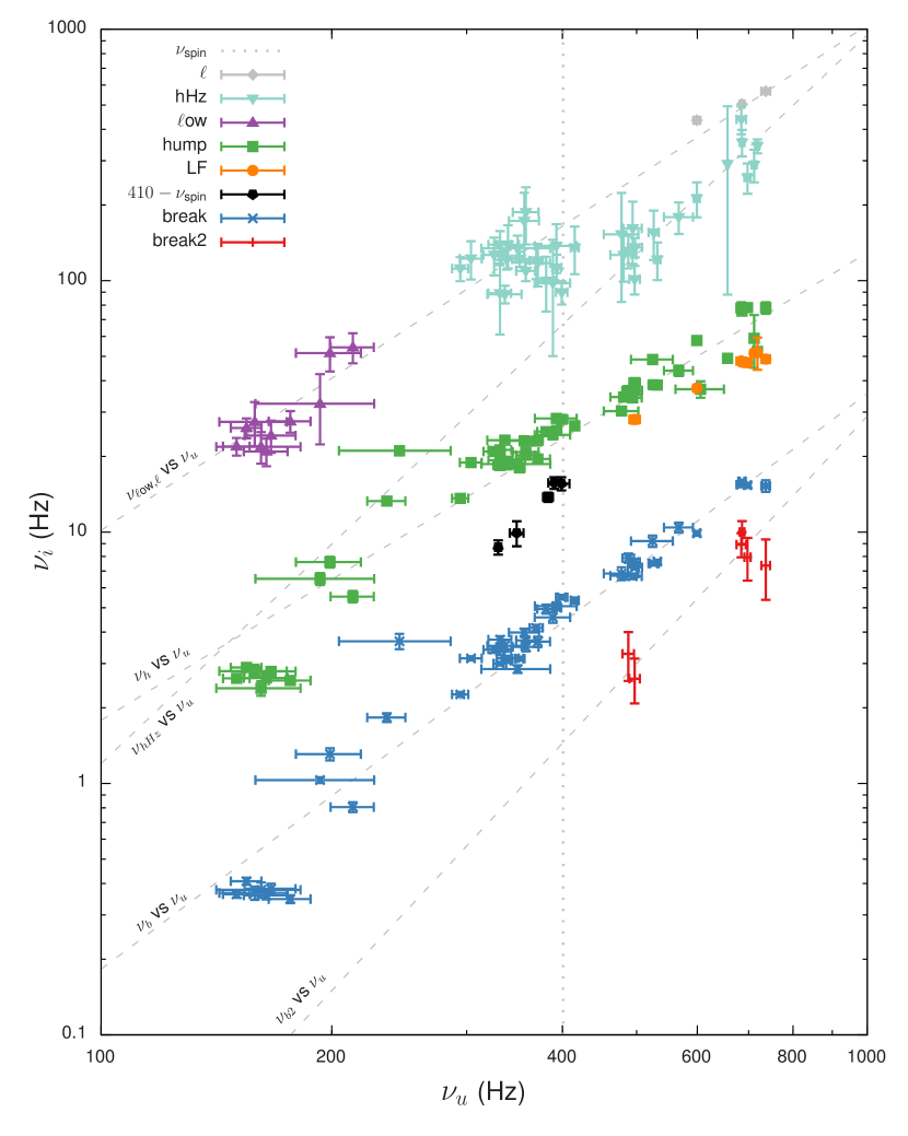
Figure 4.— Characteristic frequencies of the power spectral components as a function of $\nu_{u}$. Each point corresponds to a frequency measurement in Table 2. The dashed lines show the fitted power-law relations (see Table 7) and the vertical dotted line gives the frequency of the 401 Hz pulsations. For clarity we omitted points for which $Q_{u}$ was fixed at zero, as these points have large errors in $\nu_{u}$.

Table 7 Power-law Fit Parameters

Component	Data selection${}^{\text{a}}$	Normalization	Index	$\chi^{2}/dof$
Atoll Scheme Relations ($\nu_{i}$ vs $\nu_{u}$)
break	all	$(4.8\pm 0.7)\times 10^{-6}$	$2.29\pm 0.02$	225/47
hump	all	$(3.4\pm 0.4)\times 10^{-4}$	$1.86\pm 0.02$	748/51
hHz	$\nu_{u}>500\ {\rm Hz}$	$(2\pm 5)\times 10^{-6}$	$2.9\pm 0.4$	6/7
LF	all	$(1.2\pm 1.0)\times 10^{-3}$	$1.62\pm 0.12$	6.1/6
b2	all	$(5\pm 14)\times 10^{-9}$	$3.3\pm 0.5$	5.3/4
${\ell}\text{ow}$	all	$(1\pm 3)\times 10^{-6}$	$3.4\pm 0.8$	6/9
${\ell}\text{ow}$ & $\ell$	all	$(10\pm 2)\times 10^{-4}$	$2.01\pm 0.04$	28/12
LF & ($410-401$)	all	$(1.2\pm 0.9)\times 10^{-4}$	$1.97\pm 0.11$	58/11
State Selected Relations ($\nu_{i}$ vs $\nu_{u}$)
break & b2	EIS & all${}^{\text{b}}$	$(7\pm 2)\times 10^{-6}$	$2.17\pm 0.05$	129/15
break	IS	$(2.1\pm 0.6)\times 10^{-5}$	$2.05\pm 0.05$	110/32
hump	IS	$(1.4\pm 0.2)\times 10^{-3}$	$1.64\pm 0.02$	519/35
break	EIS	$(0.4\pm 6.6)\times 10^{-19}$	$8.6\pm 2.6$	19/9
hump	EIS	$(0.2\pm 3.5)\times 10^{-17}$	$8.2\pm 2.5$	19/9
WK relations ($\nu_{i}$ vs $\nu_{b}$)
break2	all	$(10\pm 6)\times 10^{-2}$	$1.7\pm 0.2$	1.3/4
LF	all	$7.9\pm 1.0$	$0.66\pm 0.05$	6.8/4
hump	all	$6.6\pm 0.1$	$0.88\pm 0.01$	186/54
${\ell}\text{ow}$	all	$44\pm 3$	$0.60\pm 0.09$	15/9
u	all	$208\pm 2$	$0.44\pm 0.01$	231/49
LF & ($410-401$)	all	$3.5\pm 0.7$	$0.96\pm 0.07$	83/9
PBK relations ($\nu_{i}$ vs $\nu_{{\ell}\text{ow}/\ell}$)
break	all	$(1.2\pm 0.1)\times 10^{-2}$	$1.15\pm 0.01$	215/13
hump	all	$(1.12\pm 0.01)\times 10^{-1}$	$1.04\pm 0.01$	148/12
upper kHz QPO	all	$31.2\pm 1.8$	$0.50\pm 0.01$	29/13

Note. — Results of power-law fits to the frequency-frequency relations.

5.1. Frequency Correlations

Figure 4 shows the frequency relations with respect to $\nu_{u}$ for all outbursts of SAX J1808. Overall, the measured frequencies follow the trends of the atoll correlation scheme. We quantify the relations by fitting a set of power-laws over the full $\nu_{u}$ frequency range and present the fit parameters in Table 7. We now discuss the notable features in this figure.

5.1.1 Break and Hump

The break and hump components are well correlated with $\nu_{u}$ (see Figure 4), but that correlation shows a break at $\nu_{u}\simeq 250$ Hz. This break could be due to a misidentification, however, as we are considering the three dominantly present power spectral components this is unlikely.

The break in the correlation occurs at the transition between the island state and the extreme island state and appears to affect the break and hump components in exactly the same way. Indeed, if we consider the hump frequency as a function of the break frequency (i.e. the WK relation) we find the two components are tightly correlated (Figure 5) and do not show state dependent behavior. This suggests that the break seen in Figure 4 is due to a change in $\nu_{u}$ that occurs when the source transitions between the island and extreme island states.

When considering centroid frequencies instead of characteristic frequencies, the break remains present. Additionally, for centroid frequencies the WK relation no longer holds, with $L_{h}$ drifting in frequency faster than $L_{b}$.

If the upper kHz QPO indeed shows state dependent variations that do not occur in the other components, then considering frequency correlations against $\nu_{u}$ is not optimal. In Figure 5 we therefore plot the frequencies of all components agains $\nu_{b}$ (similar to the $\nu_{\rm band}$ approach of van Straaten et al. 2002), which does not show this state dependent variation.

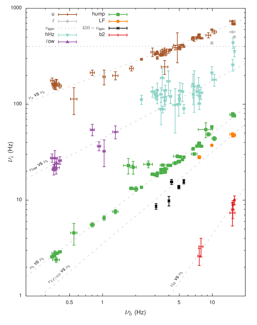
Figure 5.— Characteristic frequencies of the power spectral components as a function of $\nu_{b}$. The green squares show the hump vs break frequency (WK relation). For further details see Figure 4.

5.1.2 $L_{{\ell}\text{ow}}$ and $L_{\ell}$

The relation between $L_{{\ell}\text{ow}}$ and $L_{\ell}$ is a long standing problem. The two features were proposed to be due to the same component by Psaltis et al. (1999), who suggested that like the break and hump components, $L_{{\ell}\text{ow}}$ too becomes increasingly coherent for higher frequencies, eventually evolving into $L_{\ell}$. Plotting the frequency of $L_{h}$ against that of $L_{{\ell}\text{ow}}$ or $L_{\ell}$ then reveals a tight correlation which can be extended over three orders of magnitude by linking black hole and neutron star data.

The uncertainty of the PBK relation comes from the fact that the transition from $L_{{\ell}\text{ow}}$ to $L_{\ell}$ has never been observed. It has also been suggested that the two features are actually distinct components (van Straaten et al., 2003, 2005). For SAX J1808 specifically van Straaten et al. (2005) suggested the two components were not the same because each requires a different frequency shift to be compatible with the atoll correlation scheme.

Since most observations of SAX J1808 are in the island state, they do not have a $L_{{\ell}\text{ow}}$ or $L_{\ell}$ measurement. For those observations that do have either component present we plot the measured frequencies against $\nu_{{\ell}\text{ow}}$ and $\nu_{\ell}$ in Figure 6. The break and hump components and the upper kHz QPO all follow a correlation with $\nu_{{\ell}\text{ow}/\ell}$. Corresponding to the break below $\nu_{u}\sim 250$ Hz observed in Figure 4, the extreme island state $L_{u}$ appears to have a relatively high frequency, resulting in a flatter correlation for $L_{u}$ as compared to $L_{b}$ and $L_{h}$. The very similar correlations for $L_{b}$ and $L_{h}$ are in accordance with the idea that the $L_{{\ell}\text{ow}}$ and $L_{\ell}$ features are the same component, as assumed by PBK, and that it is $L_{u}$ that deviates at low frequency.

Based on the PBK relation (Figure 6) $L_{{\ell}\text{ow}}$ and $L_{\ell}$ could be the same, however, when considering the frequencies against $\nu_{b}$ (Figure 5) it seems more likely that $L_{{\ell}\text{ow}}$ is somehow connected to $L_{\text{hHz}}$. Whether or not the ${\ell}\text{ow}$ component and the lower kHz QPO are the same or different is therefore not clear from the SAX J1808 data alone.

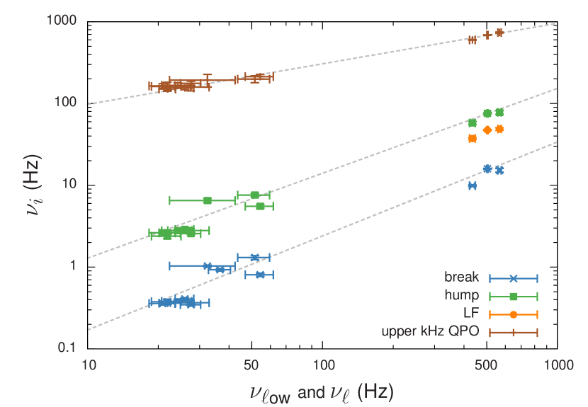
Figure 6.— Frequency measurements plotted against the $L_{{\ell}\text{ow}}$ ($<100$ Hz) and $L_{\ell}$ ($>100$ Hz) characteristic frequencies (PBK relation). Dashed lines show fitted power-law relations (see Table 7).

5.1.3 The hHz Component

The hHz component that appears in the power spectra of atoll sources is usually seen in a frequency range of 100–200 Hz and does not correlate with $\nu_{u}$ (Ford & van der Klis, 1998). Yet in SAX J1808 it appears that this hectohertz component does depend on $\nu_{u}$ (Figure 4).

For $\nu_{u}\lesssim 550$ Hz $L_{\text{hHz}}$ appears in the same way as it does in other atoll sources, showing a large scatter between 100 and 200 Hz, but remaining constant with $\nu_{u}$ (van Straaten et al., 2002, 2005). Yet from $\nu_{u}\simeq 550$ Hz the frequency of the hectohertz component starts to systematically increase with the upper kHz QPO frequency, in a way that is very similar to the trends seen in the other components.

Systematic trends of $\nu_{\text{hHz}}$ have previously been reported by Altamirano et al. (2008) who see a non-monotonic dependence of $\nu_{\text{hHz}}$ on $\nu_{u}$. These variations appear similarly for $\nu_{u}\gtrsim 550$ Hz, yet are always within the scatter of $\nu_{\text{hHz}}$ seen at lower $\nu_{u}$. In SAX J1808, however, the correlation extends well beyond the initial $\nu_{\text{hHz}}$ scatter, suggesting the trend cannot be attributed to random variations in the frequencies.

It should be noted that $L_{\text{hHz}}$ is not a dominant feature in the power spectrum. Its properties may be influenced by the position and amplitude of the nearby kHz QPOs or potentially by an unresolved ${\ell}\text{ow}$ component that could exist at similar frequencies.

The correlation between $L_{\text{hHz}}$ and $L_{u}$ was already tentatively observed by van Straaten et al. (2005), who also suggest it may be related to $L_{{\ell}\text{ow}}$. Indeed if the ${\ell}\text{ow}$ component follows the same frequency trend with $\nu_{u}$ as the break and hump components, then the island state observations should show a blend of $L_{{\ell}\text{ow}}$ and $L_{\text{hHz}}$. Then, as $\nu_{u}$ increases, the ${\ell}\text{ow}$ component could become more prominent, causing the blended feature to follow the apparent correlation with $\nu_{u}$.

If this interpretation is correct, it has a direct consequence for the relation between $L_{{\ell}\text{ow}}$ and $L_{\ell}$. In one observation, interval 4 of 2002, the supposed ${\ell}\text{ow}/\text{hHz}$ blend is seen simultaneously with a lower kHz QPO, which would imply that $L_{{\ell}\text{ow}}$ cannot be the same component as $L_{\ell}$. On the other hand, if $L_{{\ell}\text{ow}}$ and $L_{\ell}$ are in fact the same component, like the PBK relation suggests, then the observed correlation between $\nu_{\text{hHz}}$ and $\nu_{u}$ might be intrinsic to the hectohertz component. Which of these interpretations is correct remains undecided.

5.1.4 kHz QPOs

So far, twin kHz QPOs had only been reported once in SAX J1808 (Wijnands et al., 2003), from data corresponding to our interval 4 of the 2002 outburst. This frequency pair is separated by roughly half the spin frequency and is consistent with $\nu_{0,u}=|3\nu_{0,\ell}-2\nu_{\text{spin}}|$ (Wijnands et al., 2003) and a resonance at a 7:5 ratio (Kluźniak et al., 2004).

Unlike the twin kHz QPOs in most atoll sources (van der Klis, 2006), for which the lower kHz QPO is the most prominent feature, in SAX J1808 it is the upper kHz that is most prominent. This phenomenology is also seen in the AMXP XTE J1807–294 (Linares et al., 2008).

Figure 7.— Twin kHz QPO’s in SAX J1808. The top panel shows the twin kHz QPOs in interval 2 of the 2002 outburst and the bottom panel those of interval 5 in the 2011 outburst. The pulse spike at 401 Hz was excluded from the fit.

In this work we present additional detections of the twin kHz QPOs in SAX J1808 in interval 2 of the 2002 outburst and interval 5 of the 2011 outburst (Figure 4). The new detections of $L_{\ell}$ are only marginally significant ($2.8\sigma$), however, their phenomenology is entirely consistent with the original detection by Wijnands et al. (2003), providing additional evidence that we indeed observe the twin kHz QPO. All three observations are near the maximum luminosity of their respective outbursts, at a time when SAX J1808 has transitioned to the lower-left banana. The lower kHz QPO is very narrow and has a lower fractional rms amplitude than the upper kHz QPO.

Considering the centroid frequencies of all three detections of the lower kHz QPOs we find that the twin kHz QPOs move over a frequency range of about 150 Hz (see Figure 8). This trend can be fitted with a constant frequency difference of $\nu_{0,u}-\nu_{0,\ell}=(0.446\pm 0.009)\nu_{\text{spin}}$, which is inconsistent with being exactly half the spin frequency, but, being slightly smaller, may still be explained with a beat frequency model (Lamb & Miller, 2003). Alternatively the measurements may also be explained by a constant $\nu_{0,l}/\nu_{0,u}$ ratio of $1.36\pm 0.01$, close to, but inconsistent with the proposed 7:5 resonance ratio. We do note that the obtained frequency trend is tentative, as it is based on a small number of measurements and may be subject to systematic uncertainties that are not captured by the quoted errors.

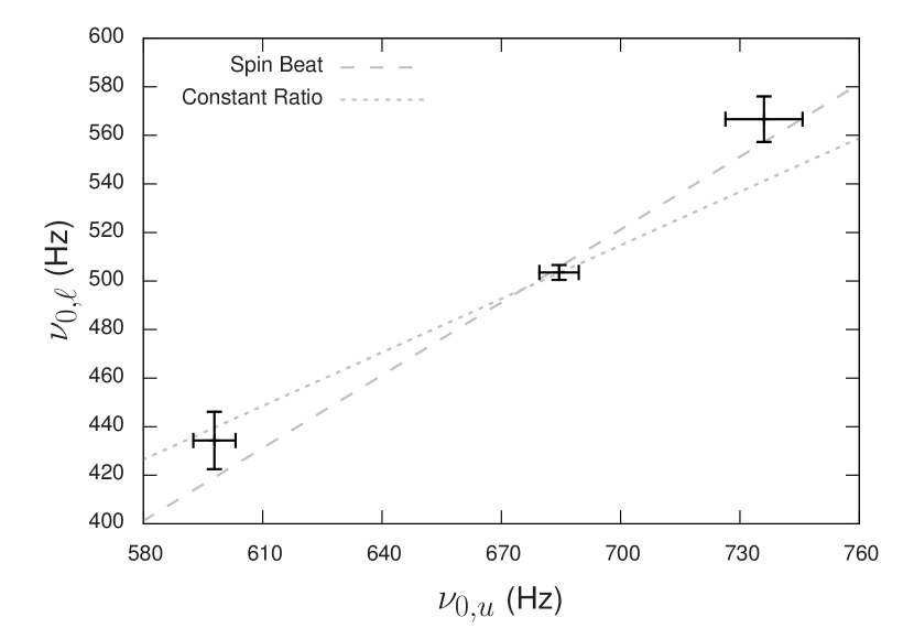
Figure 8.— Twin kHz QPO centroid frequency trend in SAX J1808. The dashed line shows the linear relation $\nu_{\ell}=\nu_{u}-0.446\nu_{\text{spin}}$, and the dotted line gives a proportionality at the constant ratio of 1.36.

5.1.5 The 410 Hz QPO

Returning to the frequency relations shown in Figure 4, we now consider the $\sim$410 Hz QPO. The characteristic frequency of $L_{410}$ correlates with the upper kHz QPO, although this relation is less steep than the others. It was noted by Wijnands et al. (2003) that the difference between the 410 Hz QPO frequency and the 401 Hz spin frequency follows a quadratic trend with $\nu_{u}$. In Figure 4 we therefore subtract the spin frequency from the measured $L_{410}$ frequency, revealing a frequency correlation for the 410 Hz QPO that is similar to that of the other components. This correlation suggests that the 410 Hz QPO is a sideband of the pulsations caused by the beat with a low frequency disk component.

Because we consider rotation frequencies, a beat signal may appear either as lower or upper sideband, depending on the relative sense of rotation. Since $L_{410}$ is observed as an upper sideband only, this suggests a beat with a quasi-periodic rotational low frequency disk phenomenon, $L_{410-401}$, that is retrograde (counter-rotates) with respect to the neutron star spin.

We searched for the associated low frequency $L_{410-401}$ component at 9 Hz in the power spectrum, both directly and using a shift-and-add method (Méndez et al., 1998), but did not detect it. Given that $L_{410}$ has a very small amplitude, it is possible that the original $\sim 9$ Hz signal is below the detection limit in this frequency region, which is dominated by the prominent $L_{b}$ and $L_{h}$ components. In the following we shall refer to the $L_{410-401}$ component keeping in mind that this inferred $\sim 9$ Hz counter-rotational disk phenomenon was not, in fact, detected as a power spectral component, but seen only as a $\sim 410$ Hz beat with the spin.

It was noticed by van Straaten et al. (2005) that the $L_{410-401}$ frequency is about half $\nu_{h}$. If we fit the relation between these two characteristic frequencies we indeed obtain a proportional relation with a slope of $0.53\pm 0.03$. Using this relation we can predict the frequency at which $L_{410}$ should appear, allowing for a shift-and-add search in the observations where $L_{410}$ is not directly observed.

In Section 4.6 we noted that $L_{410}$ is detected for $320\leq\nu\leq 401$ Hz if the source flux is greater than $\sim 40$ mCrab. We therefore first select all the low flux observations with $\nu_{u}$ in this frequency range for which $L_{410}$ was not detected. A shift-and-add search revealed a marginal feature ($2.8\sigma$) at $\nu_{\rm spin}+\nu_{h}/2$, suggesting $L_{410}$ might also present below $\sim 40$ mCrab. The observed feature has a fractional rms of $1.4$% for a fixed $Q=178$. While this quality factor is higher than the typically observed $Q\simeq 80$, it is consistent within typical errors.

A shift-and-add search for all observations with $\nu_{0,u}\geq\nu_{\rm spin}$ and a search for all observations with $\nu_{0,u}\leq 320$ Hz did not produce a detection ($<1\sigma$), giving 95% upper limits on the fractional rms of less than 1%. We note that this could either mean that the $L_{410}$ feature is not present in those observations, is too weak to be detected, or that the proposed relation with $\nu_{h}$ is not correct.

5.1.6 The LF QPO

The narrow QPO at $\sim 50$ Hz, which we labeled $L_{\text{LF}}$, was identified as such by van Straaten et al. (2005) based on extrapolating the $L_{\text{LF}}$ versus $L_{h}$ relation found in low luminosity bursters (1E 1724–3045, GS 1826–24). It was shown by Altamirano et al. (2008) that the index of this power-law is consistent with 1, implying the relation is consistent with a simple proportionality. Extending this dataset with the additional measurements from our work we find that a proportional function performs well and that the proportionality ratio is $0.65\pm 0.02$.

While the proportionality is consistent with 2/3, this small integer ratio of $L_{\text{LF}}$ with $L_{h}$ is only seen in SAX J1808, 1E 1724–3045, and GS 1826–24 (see Figure 9) and only when considering characteristic frequencies ($\nu_{max}$). Relativistic resonance models (Kluzniak & Abramowicz, 2001), which use centroid frequencies, are therefore not applicable.

While other atoll sources do not show a LF QPO that follows the same relation with $L_{h}$ we see in SAX J1808, it has been suggested that some show a sub-harmonic ($L_{\text{LF}/2}$, proportionality ratio of $0.33$) rather than $L_{\text{LF}}$ (van Straaten et al., 2005). However, many other sources have shown similar QPOs (e.g. Altamirano et al., 2005, 2008) with frequencies drifting smoothly between $L_{LF}$ and $L_{LF/2}$, crossing the frequency range of the $L_{410-401}$ component (Figure 9). This suggests $L_{\text{LF}}$, $L_{\text{LF}/2}$, and $L_{410-401}$ might be the same component.

5.1.7 LF and 410 Hz QPO

If $L_{\text{LF}}$ and $L_{410-401}$ are the same feature then this raises the question why the LF component is seen directly in the power spectrum and $L_{410-401}$ only as a sideband of the pulsations and why $L_{\text{LF}}$ and $L_{410}$ are never seen simultaneously.

The 410 Hz QPO is only observed when the upper kHz QPO centroid frequency is below the spin frequency. We recently found that when the upper kHz QPO frequency moves above the spin frequency the pulse amplitude decreases by a factor of $\sim 2$ (Bult & van der Klis, 2015). If this drop in pulse amplitude also applies to the amplitude of the beat signal, then the power of the 410 Hz QPO would drop by a factor of $\sim 4$, putting it below the detection threshold of those observations where the upper kHz QPO frequency is above the spin frequency.

As the upper kHz QPO increases further, and presumably the inner edge of the disk moves closer to the neutron star surface, neither the LF QPO nor the 410 Hz feature are observed. Finally, when source transitions to the the lower-left banana, for the highest $L_{u}$ frequencies observed in SAX J1808 and thus when the accretion disk has probably advanced closest to the neutron star surface, the LF QPO appears. If the LF QPO originates from the inner region of the accretion disk, for instance through precession, then the increased disk temperature may be the reason that the LF QPO is observed directly, while the pulsations are still too weak to power a detectable beat signal.

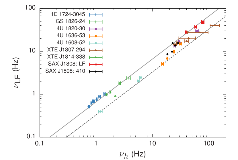
Figure 9.— Characteristic frequency of $L_{\text{LF}}$ versus $L_{h}$ for SAX J1808 and several other atoll sources. The solid line show a proportionality ratio of 0.66 and the dashed line shows a proportionality ratio of 0.33.

5.2. Precession Models

A popular interpretation of the frequency relations associates QPO frequencies with relativistic orbital and precession frequencies (Stella & Vietri, 1998, 1999). In this model the LF QPO frequency corresponds to the nodal precession frequency (or its second harmonic) of a test mass orbiting at the disk inner radius as caused by relativistic frame dragging, which in the weak field approximation is known as Lense-Thirring (LT) precession. More recent versions of this model consider the LF QPO to be caused by a geometrically thick inner flow which, also due to frame dragging, precesses as a solid body (Fragile et al., 2007; Ingram et al., 2009), and produces the correct frequencies in black hole and neutron star systems (Ingram et al., 2009; Ingram & Done, 2010), while naturally explaining a range of QPO properties (Ingram & Done, 2012).

For atoll sources specifically the relativistic precession models attribute $L_{\text{LF}}$ to LT precession. If $L_{LF}$ and $L_{410-401}$ are the same component, then the interpretation that the 410 Hz QPO arises due to a retrograde beat with the neutron star spin, implies that the precession too must be retrograde. However, LT precession is always prograde with the stellar rotation (Merloni et al., 1999; Markovic, 2000), excluding frame dragging as the main cause for the precession.

For neutron stars, however, frame dragging is not the only cause of precession. The neutron star oblateness and its magnetic field may also apply torques to the inner accretion disk, which cause a retrograde (negative) contribution to the precession frequency (Lai, 1999; Shirakawa & Lai, 2002). In the magnetic precession model the stellar magnetic field induces a warp in a geometrically thin accretion disk, which in turn undergoes retrograde precession. However, with a power-law index of $\sim 4.6$ (Shirakawa & Lai, 2002), pure magnetic precession predicts a much steeper relation with the upper kHz QPO than we observe. Classical precession (due to the oblateness), on the other hand, predicts a power-law index of $\sim 2.3$, which is closer to what we observe. It would be interesting to investigate if in neutron star systems the combination of relativistic, classical and magnetic torque contributions can produce a retrograde variant of the LT thick flow precession seen by Fragile et al. (2007) in simulations of black hole disks, with all the attractive properties gained from it.

6. Conclusions

We have presented a complete overview of the aperiodic variability of SAX J1808 as observed with RXTE over the course of 14 years. We find that SAX J1808 is mainly observed as an atoll source in the island state, and sometimes transits to the lower-left banana or the extreme island state. The individual outbursts are very similar in terms of their light curve and color evolution and, aside from the 1–5 Hz high luminosity flaring observed in 2008 and 2011, show a similar evolution of the power spectra as well.

Considering the power spectra of all outbursts we find that all characteristic frequencies are correlated with $\nu_{u}$, and that the correlations show a break when the source state changes between the island and extreme island states around $\nu_{u}\simeq 250$ Hz. This break disappears when considering the relations with $\nu_{b}$ instead, suggesting that it is $\nu_{u}$ that shows a state dependent relation with the other variability components.

We find that at $\nu_{u}\gtrsim 550$ Hz the frequency of the hHz component in SAX J1808 shows an unexpected correlation with $\nu_{u}$, that roughly follows the frequency relations of the other components. We suggest that this correlation could be due to a blend with an unresolved ${\ell}\text{ow}$ component or that it could be intrinsic to the hHz component itself. We also considered the relation between extreme island state ${\ell}\text{ow}$ component and the lower kHz QPO, but found no definitive evidence in favor or against the two being the same.

We also presented new measurements of the lower kHz QPO, which, for the first time, allows us to probe the frequency evolution of the twin kHz QPOs in this source. Our observations are consistent with a twin kHz QPO frequency separation of $(0.446\pm 0.009)\nu_{\text{spin}}$, which is inconsistent with half the spin frequency, but tentatively so, as the fit is based on a small number of measurements.

Additionally, we presented the first detailed study of the 410 Hz QPO and found that it appears only when $320\mbox{\ Hz}\leq\nu_{u}\leq\nu_{\rm spin}$. Subtracting the spin frequency from the measured $\nu_{410}$ we find that the resulting frequency matches the overall correlation trends, which strongly suggests that the 410 Hz QPO is caused by a retrograde beat against the 401 Hz spin frequency, even though the original $\sim 9$ Hz signal is never seen.

Comparing the measured hump, LF and 410 Hz beat QPO with $L_{\text{LF}}$ detections in other neutron star systems we suggest that the LF and 410 Hz beat QPOs might be the same component. We suggest this QPO might be related to retrograde nodal precession caused by the (retrograde) classical and magnetic precession dominating over the (prograde) LT precession.

References

- Altamirano et al. (2008) Altamirano, D., van der Klis, M., Méndez, M., et al. 2008, ApJ, 685, 436
- Altamirano et al. (2005) —. 2005, ApJ, 633, 358
- Belloni et al. (2002) Belloni, T., Psaltis, D., & van der Klis, M. 2002, ApJ, 572, 392
- Bult & van der Klis (2014) Bult, P., & van der Klis, M. 2014, ApJ, 789, 99
- Bult & van der Klis (2015) —. 2015, ApJ, 798, L29
- Burderi et al. (2006) Burderi, L., Di Salvo, T., Menna, M. T., Riggio, A., & Papitto, A. 2006, ApJ, 653, L133
- Campana et al. (2008) Campana, S., Stella, L., & Kennea, J. A. 2008, ApJ, 684, L99
- Dotani et al. (1989) Dotani, T., Mitsuda, K., Makishima, K., & Jones, M. H. 1989, PASJ, 41, 577
- Ford & van der Klis (1998) Ford, E. C., & van der Klis, M. 1998, ApJ, 506, L39
- Fragile et al. (2007) Fragile, P. C., Blaes, O. M., Anninos, P., & Salmonson, J. D. 2007, ApJ, 668, 417
- Galloway & Cumming (2006) Galloway, D. K., & Cumming, A. 2006, ApJ, 652, 559
- Hartman et al. (2009) Hartman, J. M., Patruno, A., Chakrabarty, D., et al. 2009, ApJ, 702, 1673
- Hartman et al. (2008) —. 2008, ApJ, 675, 1468
- Hasinger & van der Klis (1989) Hasinger, G., & van der Klis, M. 1989, A&A, 225, 79
- Ibragimov & Poutanen (2009) Ibragimov, A., & Poutanen, J. 2009, MNRAS, 400, 492
- Illarionov & Sunyaev (1975) Illarionov, A. F., & Sunyaev, R. A. 1975, A&A, 39, 185
- in ’t Zand et al. (1998) in ’t Zand, J. J. M., Heise, J., Muller, J. M., et al. 1998, A&A, 331, L25
- Ingram & Done (2010) Ingram, A., & Done, C. 2010, MNRAS, 405, 2447
- Ingram & Done (2012) —. 2012, MNRAS, 419, 2369
- Ingram et al. (2009) Ingram, A., Done, C., & Fragile, P. C. 2009, MNRAS, 397, L101
- Klein-Wolt et al. (2004) Klein-Wolt, M., Homan, J., & van der Klis, M. 2004, Nuclear Physics B Proceedings Supplements, 132, 381
- Kluzniak & Abramowicz (2001) Kluzniak, W., & Abramowicz, M. A. 2001, ArXiv Astrophysics e-prints, astro-ph/0105057
- Kluźniak et al. (2004) Kluźniak, W., Abramowicz, M. A., Kato, S., Lee, W. H., & Stergioulas, N. 2004, ApJ, 603, L89
- Lai (1999) Lai, D. 1999, ApJ, 524, 1030
- Lamb & Miller (2003) Lamb, F. K., & Miller, M. C. 2003, ArXiv Astrophysics e-prints, astro-ph/0308179
- Leahy et al. (1983) Leahy, D. A., Darbro, W., Elsner, R. F., et al. 1983, ApJ, 266, 160
- Leahy et al. (2008) Leahy, D. A., Morsink, S. M., & Cadeau, C. 2008, ApJ, 672, 1119
- Linares et al. (2005) Linares, M., van der Klis, M., Altamirano, D., & Markwardt, C. B. 2005, ApJ, 634, 1250
- Linares et al. (2008) Linares, M., Wijnands, R., van der Klis, M., et al. 2008, ApJ, 677, 515
- Markovic (2000) Markovic, D. 2000, ArXiv Astrophysics e-prints, astro-ph/0009450
- Markwardt et al. (2005) Markwardt, C. B., Swank, J., Wijnands, R., & in’t Zand, J. 2005, The Astronomer’s Telegram, 505, 1
- Markwardt et al. (2011) Markwardt, C. B., Palmer, D. M., Barthelmy, S. D., et al. 2011, The Astronomer’s Telegram, 3733, 1
- Marshall et al. (1998) Marshall, F. E., Wijnands, R., & van der Klis, M. 1998, IAU Circ., 6876, 1
- Méndez et al. (1998) Méndez, M., van der Klis, M., van Paradijs, J., et al. 1998, ApJ, 494, L65
- Menna et al. (2003) Menna, M. T., Burderi, L., Stella, L., Robba, N., & van der Klis, M. 2003, ApJ, 589, 503
- Merloni et al. (1999) Merloni, A., Vietri, M., Stella, L., & Bini, D. 1999, MNRAS, 304, 155
- Nowak (2000) Nowak, M. A. 2000, MNRAS, 318, 361
- Patruno et al. (2012) Patruno, A., Bult, P., Gopakumar, A., et al. 2012, ApJ, 746, L27
- Patruno & D’Angelo (2013) Patruno, A., & D’Angelo, C. 2013, ApJ, 771, 94
- Patruno et al. (2009) Patruno, A., Watts, A., Klein Wolt, M., Wijnands, R., & van der Klis, M. 2009, ApJ, 707, 1296
- Patruno et al. (2010) Patruno, A., Yang, Y., Altamirano, D., et al. 2010, The Astronomer’s Telegram, 2672, 1
- Poutanen & Gierliński (2003) Poutanen, J., & Gierliński, M. 2003, MNRAS, 343, 1301
- Psaltis et al. (1999) Psaltis, D., Belloni, T., & van der Klis, M. 1999, ApJ, 520, 262
- Shirakawa & Lai (2002) Shirakawa, A., & Lai, D. 2002, ApJ, 564, 361
- Stella & Vietri (1998) Stella, L., & Vietri, M. 1998, ApJ, 492, L59
- Stella & Vietri (1999) —. 1999, Physical Review Letters, 82, 17
- van der Klis (1995) van der Klis, M. 1995, in The Lives of the Neutron Stars, ed. M. A. Alpar, U. Kiziloglu, & J. van Paradijs (Dordrecht: Kluwer), 301
- van der Klis (2006) van der Klis, M. 2006, in Compact stellar X-ray sources, ed. W. H. G. Lewin & M. van der Klis (Cambridge: Cambridge University Press), 39–112
- van der Klis et al. (2000) van der Klis, M., Chakrabarty, D., Lee, J. C., et al. 2000, IAU Circ., 7358, 3
- van Straaten et al. (2002) van Straaten, S., van der Klis, M., di Salvo, T., & Belloni, T. 2002, ApJ, 568, 912
- van Straaten et al. (2003) van Straaten, S., van der Klis, M., & Méndez, M. 2003, ApJ, 596, 1155
- van Straaten et al. (2005) van Straaten, S., van der Klis, M., & Wijnands, R. 2005, ApJ, 619, 455
- Wijnands (2004) Wijnands, R. 2004, Nuclear Physics B Proceedings Supplements, 132, 496
- Wijnands et al. (2001) Wijnands, R., Méndez, M., Markwardt, C., et al. 2001, ApJ, 560, 892
- Wijnands & van der Klis (1998a) Wijnands, R., & van der Klis, M. 1998a, Nature, 394, 344
- Wijnands & van der Klis (1998b) —. 1998b, ApJ, 507, L63
- Wijnands & van der Klis (1999) —. 1999, ApJ, 514, 939
- Wijnands et al. (2003) Wijnands, R., van der Klis, M., Homan, J., et al. 2003, Nature, 424, 44
- Zhang et al. (1995) Zhang, W., Jahoda, K., Swank, J. H., Morgan, E. H., & Giles, A. B. 1995, ApJ, 449, 930