Constraints to the magnetospheric properties of T Tauri stars - II. The Mg II ultraviolet feature

Abstract

The atmospheric structure of T Tauri Stars (TTSs) and its connection with the large scale outflow is poorly known. Neither the effect of the magnetically mediated interaction between the star and the disc in the stellar atmosphere is well understood. The Mg II multiplet is a fundamental tracer of TTSs atmospheres and outflows, and is the strongest feature in the near-ultraviolet spectrum of TTSs. The International Ultraviolet Explorer and Hubble Space Telescope data archives provide a unique set to study the main physical compounds contributing to the line profile and to derive the properties of the line formation region. The Mg II profiles of 44 TTSs with resolution 13,000 to 30,000 are available in these archives. In this work, we use this data set to measure the main observables: flux, broadening, asymmetry, terminal velocity of the outflow, and the velocity of the Discrete Absorption Components. For some few sources repeated observations are available and variability has been studied. There is a warm wind that at sub-AU scales absorbs the blue wing of the Mg II profiles. The main result found in this work is the correlation between the line broadening, Mg II flux, terminal velocity of the flow and accretion rate. Both outflow and magnetospheric plasma contribute to the Mg II flux. The flux-flux correlation between Mg II and C IV or He II is confirmed; however, no correlation is found between the Mg II flux and the ultraviolet continuum or the H₂ emission.

1 Introduction

T Tauri stars (TTSs) are late type, Pre-Main Sequence (PMS) stars with masses below $\sim 2M_{\odot}$. Classical T Tauri Stars (CTTSs) are roughly solar-mass stars that are accreting gas from their circumstellar discs, whereas Weak line T Tauri Stars (WTTSs) have negligible accretion rates (see Gómez de Castro, 2013a, for a recent review).

The detection of rotationally modulated emission from hot ($\sim 10,000$ K) plasma both in the optical range (Bouvier, 1990) and in the ultraviolet (Simon et al., 1990; Gómez de Castro & Fernández, 1996) pointed out that matter in-fall is not occurring over all the stellar surface but rather it is channelled by the stellar magnetic field. TTSs photospheric magnetic fields are $\sim 1$ kG (see Johns-Krull, 2007, for a recent compilation). Assuming that T Tauri magnetospheres are predominantly bipolar on the large scale, Camenzind (1990) and Koenigl (1991) showed that the inner accretion disc is expected to be truncated by the magnetosphere at a distance of a few stellar radii above the stellar surface for typical mass accretion rates of $10^{-9}$ to $10^{-7}M_{\sun}yr^{-1}$ (Basri & Bertout, 1989; Hartigan et al., 1995; Gullbring et al., 1998). Disc material falls from the inner disc edge onto the star along the magnetic field lines, giving rise to the formation of magnetospheric accretion columns. As the free falling material in the funnel flow eventually hits the stellar surface, accretion shocks develop near the magnetic poles (see for example Romanova et al., 2012).

The ultraviolet (UV) luminosities of the TTSs exceed by 1-2 orders of magnitude those observed in main sequence stars of the same spectral types. This excess is associated with the accretion process that transports material onto the stellar surface enhancing the flux radiated by magnetospheric/atmospheric tracers, typically the ultraviolet (UV) resonance multiplets of N V, C IV, Si IV, He II, C III, C II, Si II, Fe II, Mg II, Ly-$\alpha$ and O I (see Gómez de Castro, 2009a, for a recent review of the UV properties of TTSs). Though the UV excess of TTSs is well known since the early 80’s, it is still unclear which is the dominant physical mechanism involved in its generation. There are evidences of it being produced in extended magnetospheres (Hartmann et al., 1994, 1998; Calvet & Gullbring, 1998; Gómez de Castro & Marcos-Arenal, 2012; Ardila et al., 2013; Gómez de Castro, 2013b), in accretion shocks (Gomez de Castro & Lamzin, 1999; Calvet et al., 2000; Ardila & Basri, 2000; Gullbring et al., 2000; Ardila et al., 2013; Gómez de Castro, 2013b) and in outflows (Penston & Lago, 1983; Calvet et al., 1985; Hartmann et al., 1990; Gómez de Castro & Verdugo, 2001; Coffey et al., 2007).

High resolution spectroscopy is an invaluable tool to get insight into the physics associated with the release of gravitational energy in the accretion process. Emission from jets, discrete absorption components (DACs) from accreting cloudlet or episodic ejections and the radiation from the large scale excitation of the magnetosphere by the infalling gas, can be best disentangled by their kinematical signature. The Mg II resonance multiplet UV1 is the strongest line in the UV spectrum of TTSs, only surpassed by the Ly-$\alpha$ line that it is often strongly absorbed by the circumstellar material. The extended neutral outflow absorbs strongly the blue wind of the Ly-$\alpha$ line. Moreover, the molecular hydrogen in the circumstellar environment absorbs Ly-$\alpha$ photons that produce the H₂ fluorescent emission detected in the UV (Herczeg et al., 2002; France et al., 2012). Compared with Ly-$\alpha$, Mg II has the advantage of sampling a narrower temperature range preventing the pollution from the diffuse emission/absorption from the cool extended H I envelopes. Note that the ionization potentials of Mg I and Mg II are 7.65 eV and 15.03 eV, respectively; henceforth Mg II is a tracer of plasmas in the temperature range from some few thousand Kelvin up to $\sim 20,000$ K. Moreover, the Mg II[uv1] electronic levels distribution permits to treat the ion as a two levels specie allowing a simple treatment of the radiation transfer (see Catala et al., 1986).

From the observational point of view, the Mg II lines have the advantage of their high Signal-to-Noise Ratio (S/N); the multiplet is observed at $\lambda\lambda 2796,2804$ Å vacuum wavelength, where the sensitivity of the UV instrumentation is high, allowing to obtain high resolution profiles even with small effective area telescopes such as the International Ultraviolet Explorer (IUE) (Penston & Lago, 1983; Calvet et al., 1985; Gómez de Castro, 1998; Ardila et al., 2002; Herczeg et al., 2004). For this reason, there is a large enough sample of observations to run a study of the TTSs as a class, including variability. The objective of this work is to run such a study.

The Mg II lines have been used by several authors to study the structure of some few TTSs and to derive different physical properties (see e.g. Imhoff & Giampapa, 1980; Gómez de Castro & Franqueira, 1997; Lamzin, 2000). Giampapa et al. (1981) used a sample of 13 TTSs observed with the IUE to study the chromospheric origin of the Mg II emission and to derive the mass loss rates in the TTSs’ wind. Further research on the connection between the chromosphere and the extended envelope was carried out by Calvet et al. (1985), who made use of simultaneous observations of the Ca II and Mg II lines of BP Tau, DE Tau, RY Tau, T Tau, DF Tau, DG Tau, DR Tau, GM Aur SU Aur, RW Aur, CO Ori and GW Ori to conclude that the chromospheric structure seemed to be related with the mass of the stars. TTSs with masses above 1.5 M_⊙ seemed to produce the Mg II emission in extended envelopes, alike the H$\alpha$ emission, while less massive TTSs have Mg II emission produced in the chromosphere. This result was interpreted in terms of the internal structure of the star and the energy transport. Low mass, fully convective, TTSs were expected to be slower rotators. However, the authors concluded that Mg II emission also seemed to be produced in extended regions in some low mass TTSs. Ardila et al. (2002) analysed the relationship between the Mg II flux and several stellar properties using a small sample of TTSs (those observed with the Goddard High Resolution Spectrograph (GHRS) in Hubble Space Telescope (HST)). The sample included: BP Tau, T Tau, RW Aur, DF Tau, DG Tau, RU Lup, RY Tau, T Tau, DR Tau and HBC 388. However, no correlation between the Mg II flux and the accretion rate was found. Also, they did not find any correlation between any parameter of the Mg II line emission and the inclination. This result was interpreted by the authors as an evidence of the line emission coming from a non-occulted area. However, evidence of a latitude dependent wind was claimed from the data. Finally the comparison between the H$\alpha$ emission and the Mg II emission of BP Tau, DF Tau, RW Aur and DR Tau (the observations were not simultaneous) pointed out that the line broadening were very similar indicating that line broadening was dominated by the kinematics of the emission region rather than by other mechanisms, i.e. stark broadening. The relation between the Mg II flux and the accretion rate is at debate. Calvet et al. (2004) showed that Mg II line luminosity correlates with accretion luminosity in accreting stars and the same trend was found using spectra obtained with the Space Telescope Imaging Spectrograph (STIS) by Ingleby et al. (2011). However, this correlation was found on the basis of low resolution data and as pointed out in earlier works the Mg II doublet is saturated.

The Mg II emission is a main tracer of the TTSs magnetosphere and its study is fundamental to determine its extent and heating sources. In a previous work, we estimated the plasma properties in the formation region of the semi-forbidden C II], Fe II] and Si II] lines. In that work we pointed out that these lines are formed in the accretion flow. In three stars (DG Tau, FU Ori and RY Tau) a contribution of the outflows to the lines was observed, suggesting that the properties in the base of the jet are similar to those observed in the base of the accretion stream (López-Martínez & Gómez de Castro, 2014). As the TTSs magnetosphere is expected to end in a sheared boundary layer, acting as the magnetized interface with the Keplerian disc, understanding the source of the Mg II lines broadening can provide fundamental clues on the star-disc angular momentum transport. Currently, there are in the IUE and HST archives observations of the Mg II line profiles with resolutions between 15,000 and 45,800 of 44 TTSs, including WTTSs, fast and slow rotators with a large range of ages and masses. This provides a extraordinary sample to run statistically significant tests on the properties of the TTSs and the evolution of their magnetosphere as they approach the main sequence. In this work, we analyse 126 observation of 44 TTSs to run such a study. For most of them, also the Ly-$\alpha$ profile is available in the HST archive. This information has been used to complete the view on the circumstellar environment of the TTSs. The Archive data are described Sect. 2. The characteristics of the sample of TTSs observed by these missions are summarized in Sect. 3. Since there are many uncertainties in the PMS evolutionary tracks, age and masses have been derived for all sources. The data and the measurement procedures are described in Sect. 4. In Sect. 5, the constraints to the physics of the TTSs outflows are analysed from the data. The connection between accretion process and line emission is re-examined on the light of the new data in Sect. 6. The article concludes with a summary in Sect. 7.

2 Archival data

The Mg II profiles were extracted from the IUE and HST archives for the log of observations shown in Table 1. We checked the archives for all the available observations of the Mg II profiles for TTSs with resolutions between 13,000 and 30,000. Taking into account these characteristics, we selected 126 observations of 44 TTSs the archives.

Table 1: Telescope/instrument details of the Mg II observations of the stars in the sample. The full table is available online as Supporting Information.

Star	Instrument	Obs. Date	Data set	Res.	Exposure	S/N
		(yy-mm-dd)	Id.	power	Time (s)
AA Tau	HST/STIS	07-11-01	ob6ba7030	30000	1462.2	4.20
AK Sco	IUE	86-08-06	LWP08847	13000	16859.8	7.80
	IUE	88-04-01	LWP12964	13000	5099.8	very noisy
	IUE	88-04-02	LWP12967	13000	33599.6	5.40
	IUE	88-04-02	LWP12968	13000	9899.5	3.10
	IUE	88-04-09	LWP13006	13000	25799.8	8.30
	HST/STIS	10-08-21	ob6b21030	30000	1015	13.90
BP Tau	IUE	81-07-24	LWR11130	13000	12599.6	8.60
	IUE	85-10-22	LWP06963	13000	10799.8	very noisy

The IUE observations were obtained in high dispersion mode with R$\simeq$13,000. The Mg II lines were in orders 82 and 83 in the long wavelength spectrograph. The Mg II h (2796 Å) line is well centred in order 82 but the Mg II k (2803 Å) line was at the edge of the orders. The echelle ripple correction introduced an enhancement of the noise, as a result the Mg II k line is more noisy and shows some spikes in the IUE spectra. This problem was partially solved in the final IUE data processing both for NEWSIPS (New Spectral Image Processing System) and INES (IUE Newly Extracted Spectra). NEWSIPS release is accessible trough the MAST archive (see Nichols & Linsky, 1996, for details in the IUE data processing). In the INES database, also the high resolution ’concatenated’ spectra are stored. In the INES release the spectral orders are connected, eliminating the regions overlapped through a procedure designed to optimize the S/N at the edges of the orders (see Cassatella et al., 2000, for details). A comparison between both releases can be found in González-Riestra et al. (2000). The data used in this article were retrieved from the INES archive.

The HST observations were obtained with three different instruments: GHRS, STIS and the Cosmic Origins Spectrograph (COS). The details on the instrument, grating, aperture, dispersion for each instrument and configuration are provided in the log of observations for each data set. Some of the observations obtained with STIS are included in the catalogue of UV stellar spectra of cool stars: CoolCat. In this case, the data were retrieved directly from the CoolCat web site (see Ayres, 2010, for details). There are repeated observations of up to 17 stars in the sample, allowing to study the profiles variability.

The Ly-$\alpha$ profiles were extracted from the HST archive. The observations were obtained either with STIS (E140M; G140M) or with COS (G130M) (see Table 7).

The lines profiles are plotted in Fig. 1. The profiles are arranged in increasing order of line broadening and asymmetry. This is also the sequence from WTTSs to heavily accreting TTSs. In the last panel, three stars: CY Tau, DM Tau and AK Sco are plotted. These are accreting sources where the red-wards shifted wing of the profile is more absorbed than the blue-wards shifted one.

Most of the Ly-$\alpha$ profiles are dominated by the geocoronal emission. In the STIS spectra, it is observed as a narrow emission component at rest wavelength. However, in the COS spectra, the geocoronal emission is much broader because of the wider aperture (see France et al., 2012, for details on the Ly-$\alpha$ profiles of the TTSs obtained with COS). As a result, the only relevant information about the Ly-$\alpha$ profile of the TTSs concerns the high velocity wings of the line. For this reason, the Ly-$\alpha$ profiles are plotted in logarithmic scale. The absorption of Ly-$\alpha$ photons by the circumstellar neutral wind is readily observed; there is also Ly-$\alpha$ absorption by the H₂ molecules in the circumstellar environment, that has been used to reconstruct the underlying Ly-$\alpha$ profile (see Herczeg et al., 2004; Schindhelm et al., 2012).

The FUV data used in this work (C IV, He II and H₂) have been taken from Ardila et al. (2013); Gómez de Castro (2013b); France et al. (2012), respectively. Most of the targets were observed with STIS (E140M) and COS (G130M; G160M).

Figure 1: Ly-$\alpha$ and Mg II profiles of the TTSs. The Ly-$\alpha$ profiles are plotted in logarithmic scale to show in detail the wings since the core of the line is spurious geocoronal Ly-$\alpha$ emission.

Figure 2: continued

3 General properties of the sample

The sample covers a broad range of stellar and disc properties as summarized in Table 2, such as Spectral Type (S.T.), distance (d), inclination (i), extinction value (A_V), accretion rate ($\dot{M}$) and stellar rotation ($v{\rm sin}(i)$).

Table 2: Properties of the stars analysed in this work.

Star	S.T.	d	$i$	$A_{V}$	$\dot{M}(M_{\sun}yr^{-1})$	$v{\rm sin}(i)$	$\log(T_{eff}/K)$	$\log(L/L_{\sun})$	$M$	Age
		(pc)	(deg)	(mag)	($\times 10^{-8}$)	(km/s)			$(M_{\sun})$	(Myr)
AA Tau	K7 (24)	140	75 (18)	1.9 (24)	1.50 (24)	11 (1)	3.58 (32)	-0.19 (32)	0.4	0.6
AK Sco	F5 (12)	145	65-70 (12)	0.5 (12)	-	18.5 (12)	3.81 (3)	0.82 (31)	1.5 (a)	20.0
BP Tau	K7 (24)	140	30 (18)	1.1 (24)	2.90 (24)	10 (1)	3.61 (19)	-0.19 (19)	0.5	1.1
CS Cha	K6 (24)	160	60 (18)	0.3 (24)	0.53 (24)	21 (3)	3.64 (3)	0.43 (3)	0.6	0.3
CV Cha	G9 (24)	160	35 (10)	1.5 (24)	5.90 (24)	32 (3)	3.74 (3)	0.90 (3)	3.0	1.5 (a)
CY Tau	M2 (4)	140	47 (25)	0.03 (4)	0.14 (4)	10.6 (15)	3.57 (19)	-0.40 (19)	0.4	1.1
DE Tau	M2 (24)	140	35 (18)	0.9 (24)	2.80 (24)	10 (1)	3.55 (3)	-0.04 (3)	0.3	0.1
DF Tau	M1 (4)	140	80 (6)	0.15 (4)	1.00 (4)	16.1 (27)	3.57 (19)	-0.33 (19)	0.4	0.8
DG Tau	K6 (4)	140	90 (7)	1.41 (4)	4.60 (4)	20 (3)	3.62 (30)	-0.55 (30)	0.8	9.0
DI Cep	G8IV (13)	300	-	0.24 (13)	$\ga$0.6 (13)	23.5 (37)	3.74 (3)	0.71 (3)	2.0	3.0
DK Tau	K7 (24)	140	50 (18)	1.3 (24)	3.40 (24)	11.5 (1)	3.61 (19)	-0.05 (19)	0.5	0.6
DM Tau	M1 (24)	140	35 (18)	0.7 (24)	0.29 (24)	4 (15)	3.57 (19)	-0.80 (19)	0.6	7.0
DN Tau	M0 (24)	140	28 (18)	0.9 (24)	1.00 (24)	12.3 (15)	3.59 (19)	-0.10 (19)	0.4	0.5
DR Tau	K5 (24)	140	72 (18)	1.4 (24)	5.20 (24)	10.0 (3)	3.61 (19)	0.29 (19)	0.4	0.2
DS Tau	K5 (4)	140	90 (25)	0.9 (4)	1.20 (4)	10.0 (1)	3.69 (3)	-0.22 (3)	1.1	12.0
FM Tau	M0 (24)	140	-	0.7 (24)	0.12 (24)	-	3.50 (32)	-0.65 (32)	0.1	0.3
FU Ori	G0 (38)	450	40 (8)	-	-	-	-	-	-	-
GM Aur	K7 (24)	140	55 (18)	0.6 (24)	0.96 (24)	12.4 (27)	3.68 (19)	0.09 (19)	1.0	2.5
GW Ori	G0 (26)	450		1.3 (26)	27.00 (26)	40 (26)	3.75 (3)	1.82 (3)	3.0	1.0 (a)
HBC 388(W)	K1 (4)	140	45 (6)	0 (4)	0.40 (4)	19.5 (16)	3.71 (2)	0.15 (2)	1.4	5.0
HBC 427(W)	K5 (17)	140	67 (20)	0 (17)	-	-	3.64 (20)	-0.12 (20)	0.7	1.9
HN Tau	K5 (24)	140	45 (18)	1.1 (24)	1.40 (24)	52.8 (27)	3.60 (32)	-0.56 (32)	0.7	6.0
IP Tau	M0 (24)	140	60 (18)	1.7 (24)	0.72 (24)	12.3 (15)	3.58 (19)	-0.36 (4)	0.5	1.5
LkCa 4(W)	K7 (4)	140	-	1.21 (4)	0.19 (4)	30 (15)	3.61 (19)	-0.13 (19)	0.5	0.9
LkCa 19(W)	K0 (4)	140	-	0.74 (4)	0.01 (4)	21 (3)	3.72 (19)	0.19 (19)	1.4	9.0
PDS 66	K1 (24)	86	30 (22)	0.2 (24)	0.01 (24)	14 (21)	3.70 (35)	0.00 (35)	1.2	7.0
RECX 1(W)	K4 (25)	97	-	0 (25)	-	22 (21)	3.63 (21)	0.00 (24)	0.6	0.8
RECX 15	M3 (24)	97	60 (18)	0 (24)	0.08 (24)	15.9 (28)	3.53 (28)	-1.07 (28)	0.3	5.0
RECX 11	K5 (24)	97	70 (18)	0 (24)	0.02 (24)	16.4 (29)	3.65 (34)	-0.22 (24)	0.9	4.0
RU Lup	K7 (17)	140	24 (11)	0.1 (17)	-	9 (11)	3.61 (30)	-0.38 (30)	0.6	2.8
RW Aur	K3 (24)	140	40 (6)	0.5 (24)	2.00 (24)	15 (3)	3.66 (19)	0.24 (19)	0.8	0.8
RY Tau	G1 (9)	140	86 (5)	2.2 (9)	6.80 (9)	48.7 (1)	3.71 (19)	0.82 (19)	1.9	2.4 (a)
S CrA	K6 (3)	130	-	0.5 (3)	-	-	3.63 (3)	0.11 (3)	0.6	0.5
SU Aur	G1 (9)	140	86 (5)	0.9 (9)	4.90 (9)	59 (15)	3.77 (19)	0.97 (19)	2.0	6.3 (a)
SZ 102	K0 (25)	200	10 (18)	0.32 (25)	0.79 (25)	-	3.72 (23)	-1.94 (23)	-	-
T Tau	K0 (4)	140	20 (6)	1.46 (4)	3.20 (4)	20.1 (1)	3.72 (3)	0.90 (3)	2.0	1.8 (a)
TW Hya	K7 (24)	56	7 (7)	0 (24)	0.18 (24)	5.8 (7)	3.61 (30)	-0.77 (30)	0.8	20.0
TWA 7(W)	M1 (17)	27	28 (14)	0 (17)	-	4 (21)	3.52 (14)	-0.49 (33)	0.2	0.3
TWA 3A	M3 (24)	50	-	0 (24)	0.01 (24)	12 (21)	3.53 (21)	-1.10 (17)	0.3	5.0
TWA 13A (W)	M1 (17)	53	-	0 (17)	-	12 (21)	3.56 (36)	-0.79 (33)	0.5	6.0
UX Tau	K5 (4)	140	35 (18)	0.26 (4)	1.10 (25)	25.4 (39)	3.64 (19)	0.11 (19)	0.7	0.7
V819 Tau(W)	K7 (4)	140	-	1.64 (4)	0.14 (4)	9.1 (15)	3.60 (32)	-0.13 (32)	0.5	0.7
V836 Tau	K7 (24)	140	65 (18)	1.5 (24)	0.11 (24)	13.4 (15)	3.61 (30)	-0.49 (30)	0.7	5.0

(a) Values taken from other authors because they could not be measured from D’Antona & Mazzitelli (1997) tracks.

(W) WTTSs of the sample according to the references indicated in this table.

(1) Hartmann et al. (1986); (2) Kundurthy et al. (2006); (3) Johns-Krull et al. (2000); (4) White & Ghez (2001); (5) Muzerolle et al. (2003); (6) Ardila et al. (2002); (7) Herczeg et al. (2006); (8) Hartmann et al. (2004); (9) Salyk et al. (2013); (10) Hussain et al. (2009); (11) Stempels et al. (2007); (12) Gómez de Castro (2009b); (13) Gómez de Castro & Fernández (1996); (14) Yang et al. (2008); (15) Nguyen et al. (2009); (16) Sartoretti et al. (1998); (17) Yang et al. (2012); (18) France et al. (2012); (19) Bertout et al. (2007); (20) Steffen et al. (2001); (21) da Silva et al. (2009); (22) Sacco et al. (2012); (23) Hughes et al. (1994); (24) Ingleby et al. (2013); (25) Ardila et al. (2013); (26) Calvet et al. (2004); (27) Clarke & Bouvier (2000); (28) Woitke et al. (2011); (29) Jayawardhana et al. (2006); (30) Herczeg & Hillenbrand (2008); (31) Manoj et al. (2006); (32) Hartigan et al. (1995); (33) Ingleby et al. (2011); (34) Lawson et al. (2001); (35) Mamajek et al. (2002); (36) Sterzik et al. (1999); (37) Azevedo et al. (2006); (38) Petrov & Herbig (2008); (39) Preibisch & Smith (1997).

3.1 Age and mass

Age and mass determinations for TTSs are uncertain. Published measurements of TTSs luminosities and effective temperatures (see Table 2) were used to compute the masses and ages provided in the last two columns of Table 2.

First, we used the D’Antona & Mazzitelli (1997) evolutionary tracks (see Fig. 3, top panel). This model introduces a Kolmogorov based turbulence cascade (Canuto & Mazzitelli, 1991) in the parametrisation of the internal stellar heat transport. According to these tracks, our sample covers the age range from 1 to 10 Myr and a broad range of masses, from 0.2 to 2 M_⊙.

Secondly, we used the Siess et al. (2000) evolutionary tracks (see Fig. 3, bottom panel). These evolutionary tracks do not include a complex treatment of transport but take into account the effect of fresh deuterium accretion in PMS evolution. According to these tracks, the range of masses of the stars in our sample is reduced with respect to the D’Antona’s tracks but the spread in age is increased notably: from 3 to 30 Myr.

Finally, in Fig. 4, masses are compared for both sets of estimates. Note that the mass calculations are rather robust, i.e., both sets of evolutionary tracks provide similar results. We also compared the ages for both PMS evolutionary tracks. We found a large discrepancy in the age estimates. These masses and ages values are provided in the last two columns of Table 2.

Figure 3: Location of the TTSs on the D’Antona & Mazzitelli (1997) (top) and Siess et al. (2000) (bottom) PMS evolutionary tracks. Triangles represent WTTSs.

Figure 4: Comparison of the mass estimates obtained using D’Antona & Mazzitelli (1997) and Siess et al. (2000) PMS evolutionary tracks. The dashed line represents $M_{D^{\prime}Antona}=M_{Siess}$.

3.2 Binaries

There are several binaries and multiples in the sample: RY Tau (Bertout et al., 1999), AK Sco (Andersen et al., 1989), DF Tau (Bertout et al., 1988; Bouvier et al., 1993; Unruh et al., 1998), GW Ori (Mathieu et al., 1991), CV Cha (Bertout et al., 1999; Hussain et al., 2009), RW Aur (Bertout et al., 1999; White & Ghez, 2001), S CrA (Walter & Miner, 2005), DK Tau, HN tau (Correia et al., 2006), UX Tau, V819 Tau (Nguyen et al., 2012), FU Ori (Wang et al., 2004), RECX 1, HBC 427, CS Cha (Ardila et al., 2013) and T Tau (Furlan et al., 2006; Herbst et al., 1996).

Four of them, namely RY Tau, AK Sco, DF Tau and GW Ori are close binaries with semi-major axes 3.17, 0.14, 12.6 and 1 AU, respectively. Henceforth the contribution from the components is unresolved in the IUE and HST/GHRS profiles.

The distances between the components in the CV Cha, S CrA, RW Aur, DK Tau, HN Tau, UX Tau, FU Ori, T Tau, RECX 1, HBC 427 and V819 Tau are $11.4$, $1.3$, $1.4$, $2.3$, $3.1$, $5.9$, $0.5$, $0.7$, $0.18$, $0.03$ and $10.5$ arcsec, respectively. RW Aur, UX Tau (Nguyen et al., 2012), RECX 1, T Tau (Ardila et al., 2013), and GW Ori (Berger et al., 2011) are multiple systems.

3.3 Optical jets sources

RY Tau (St-Onge & Bastien, 2008), RW Aur (White & Ghez, 2001; Coffey et al., 2008), DG Tau (White & Ghez, 2001; Coffey et al., 2008), and T Tau (Furlan et al., 2006; Herbst et al., 1996) are sources of resolved jets. The inclinations of the jets of DG Tau and RW Aur with respect to the plane of the sky have been estimated to be $52^{\circ}$ and $44^{\circ}$, respectively. DG Tau jet is well collimated with knots and bow shocks out to at least $11$ arcsec, with velocities of several 100 Km s^-1 (Güdel et al., 2008). The Mg II emissions from RW Aur, HN Tau, DP Tau and CW Tau jets have been measured (Coffey et al., 2012). The Mg II lines are roughly 1-2 orders of magnitude stronger than the optical forbidden lines and, in general, the approaching jet is brighter than the receding jet, as otherwise expected by the impact of circumstellar extinction and the absorption by the intervening warm environment. The (unresolved) jet contribution to the Mg II profile is shown in the high velocity edge of the profile (see Coffey et al., 2008).

3.4 Magnetic fields and spots

Strong magnetic fields have been directly detected in CTTSs. Magnetic fields of kilo-Gauss (kG) have been measured from Zeeman broadening measurements only for few sources: AA Tau (2.78 kG), BP Tau (2.17 kG), CY Tau (1.16 kG), DE Tau (1.12 kG), DF Tau (2.90 kG), DG Tau (2.55 kG), DK Tau (2.64 kG), DN Tau (2.00 kG), GM Aur (2.22 kG), T Tau (2.37 kG) and TW Hya (2.61 kG) (Johns-Krull, 2007). Indications of strong magnetic activity or magnetic channelled accretion have been found in some other sources.

The study of the Zeeman broadening analysis and measurement of the circular polarization signal allows to derive the field topology itself. Magnetic surface maps have been published for several accreting TTSs derived from the technique of Zeeman-Doppler imaging (see, for instance, Donati et al., 2007, 2008, 2012; Hussain et al., 2009; Gregory et al., 2012). We use for CV Cha the magnetic field derived with this technique: $>0.02$ kG.

Hot spots on the stellar surface are produced by accretion shocks and they have been detected in BP Tau (Gómez de Castro & Franqueira, 1997; Johns-Krull et al., 2004; Donati et al., 2008), CY Tau (Bouvier et al., 1995), DF Tau (Bertout et al., 1988; Bouvier et al., 1993; Unruh et al., 1998) and DI Cep (Gómez de Castro & Fernández, 1996).

4 Measurements and data analysis

Fig. 1 shows a trend of increasing Mg II strength and profile broadening from WTTSs to classical TTSs. There is not a clear cut separation between the two groups. Rather, it seems there is a sequence associated with the line emitting volume and the strength of the wind. The correlation between broadening and strength has been already noticed for other spectral tracers, such as the C IV or the N V lines, most recently by Ardila et al. (2013); Gómez de Castro (2013b). This sequence is also associated with the weakening of the H₂ molecular emission and the evaporation of the gas in the circumstellar disc.

Let us follow the trend outlined in Fig. 1. The Mg II profiles of the WTTSs are rather narrow (typical widths at the base of the line are $\sim 160.5$ km s^-1) with a circumstellar absorption feature over the TTS line emission. It is noticeable that the feature is at rest with respect to the star’s emission only in HBC 427 and V819 Tau. In LkCa 19 and LkCa 4, it is slightly red-wards shifted and in the rest of the sources blue-wards shifted. Given the strength of the feature and the location of our sample stars (at distances smaller than 200 pc from the Sun for the majority of the sources), the feature is expected to be produced by warm absorbing circumstellar material. These slight shifts suggest a mainly outflow motion in the circumstellar environment along the line of sight.

The comparison with the Ly-$\alpha$ profiles also shows the uncertainties of a morphologically based classification in terms of the Mg II profile. The Ly-$\alpha$ profiles of the WTTSs (LkCa 4, LkCa 19 and HBC 427) are narrow enough to be fully covered by the geocoronal Ly-$\alpha$ emission; no high velocity wings are detected (see Fig. 1). However, TTSs with apparently similar Mg II profiles, such as FM Tau, TWA 7, TWA 13A, RECX 1, RECX 11 display broad wings in Ly-$\alpha$.

Mg II profiles in CTTSs can be described as a broad emission with significant wind absorption in the blue wing (in addition to the narrow circumstellar feature). The high S/N of the HST observations permit to follow the velocity law in the wind and its geometry. The strength of the wind varies significantly from source to source and, in some objects like GM Aur, two broad absorption components (winds?) are observed. There are three peculiar profiles in the sample: BP Tau, RW Aur and AK Sco. There is not significant wind absorption in BP Tau. RW Aur profile is extremely broad; this fact is even noticeable in tracers like the C III] and Si III] semi forbidden transitions and drove Gómez de Castro & Verdugo (2003) to hypothesize the existence of an ionized plasma torus around this star. AK Sco is the only star displaying a broad red-wards shifted absorption but this is caused by the complex circumstellar gas dynamics in this close binary system (see the numerical simulations in Gómez de Castro et al., 2013c). In the following, we describe the procedures followed to quantify the evolution of the profiles and the characteristics of the outflows.

4.1 Mg II flux measurements and flux-flux correlations

The flux radiated in the Mg II lines is calculated as $F_{a,b}=(\sum_{i=0}^{i=n_{a,b}}F_{a,b}(\lambda_{i})-n_{a,b}<C>)*\delta\lambda,$ being $\lambda_{0,a}$ and $\lambda_{0,b}$ the short wavelength edges of the 2796 Å and 2804 Å Mg II lines (subscripts ’a’ and ’b’, respectively). $\delta\lambda$ is the pixel size, $\lambda_{i}=\lambda_{0}+i*\delta\lambda$ and $n_{a,b}$ the number of pixels in each profile. The average continuum level $<C>$ was determined in one nearby, featureless, window and the dispersion about this average, $\sigma$, is used to compute the flux errors as $dF_{a,b}=\sigma n_{a,b}$ (see below for the determination of the profile edge). These flux errors are represented in figures with error bars. For the measured velocities we took an error of 1 Å for all stars. Since the stellar bolometric, $F_{bol}$, is $F_{bol}=(\sigma T^{4}4{\rm\pi}R_{*}^{2})/4{\rm\pi}d^{2}$, the rate $F_{l}/F_{bol}$, with l the corresponding line, provides a measure of the line emissivity corrected from stellar radii and surface temperature. In this manner, the normalised fluxes are corrected from scaling effects associated with the broad range of mass, luminosity and stellar radius covered by the TTSs sample studied in this work.

As shown in Fig. 5, the ratio $F_{2796}/F_{2804}<2$ in most sources; the line is optically thick both in WTTSs to CTTSs. The average value is $1.4\pm 0.2$. Thus, though the 2796 Å line is saturated in all sources, the 2804 Å line may be not it in many observations. For this reason, all tests for flux scaling with other parameters are carried out using the 2804 Å line. The 2795 Å line will only be used in this article to determine some kinematical properties of the outflow that are not affected by the saturation. Note that this also means that scaling based on Mg II fluxes determined from low dispersion data should be treated with care.

All line fluxes are provided in Table 3. Fluxes were extinction corrected using Valencic et al. (2004) extinction law (assuming $R_{V}=\frac{A_{V}}{E(B-V)}=3.1)$ and the $A_{V}$ values in Table 2. Note that there are large differences in the extinctions quoted by different authors (compare for instance Ingleby et al., 2011; Yang et al., 2012). We estimate that extinctions are uncertain by $\leq 0.5$ mag which corresponds to a flux uncertainty by a factor $\leq 1.5$.

From Table 3, it can be readily inferred variations in the line flux by factors of $\sim 5$ over the years. This is observed in all the TTSs for which there are several observations available. In Fig. 6 we have represented those being observed more than three times. Note that the typical observing times are long (see Table 1), so flares and eruptive events can be excluded in most cases.

Figure 5: The 2796/2804 flux ratio, as a function of the flux of the Mg II($\lambda$ 2804 Å) line. WTTSs are represented by triangles.

Table 3: Mg II flux measurements corrected from extinction and velocity measurements of the analysed profiles.

		Flux Measurements				Velocity Measurements
Star	Date	$F_{2796}$	$F_{2804,b}$	$F_{2804,r}$		$V_{term}$	DACs	Comments
	(yy-mm-dd)	($10^{-12}erg\ s^{-1}\ cm^{-2}$)				(km/s)
AA Tau	07-11-01	$1.93\pm 0.46$	$0.63\pm 0.28$	$0.74\pm 0.26$		-50.0		narrow
AK Sco	86-08-06	$3.04\pm 0.39$	$1.35\pm 0.17$	$0.76\pm 0.22$			129.8	no absorption
	88-04-02	$3.20\pm 0.59$	$0.92\pm 0.20$	$0.45\pm 0.25$				no absorption
	88-04-02	$2.37\pm 0.75$	$0.79\pm 0.33$	$0.38\pm 0.32$				no absorption
	88-04-09	$4.01\pm 0.48$	$1.16\pm 0.18$	$1.17\pm 0.23$				no absorption
	10-08-21	$3.86\pm 0.28$	$1.60\pm 0.11$	$0.87\pm 0.16$				no absorption
BP Tau	81-07-24	$15.40\pm 1.79$	$4.79\pm 0.68$	$6.74\pm 1.39$		-213.0		variable
	86-10-10	$12.11\pm 2.30$	$0.08\pm 0.06$	$8.98\pm 1.44$		-237.7		variable
	86-10-26	$5.98\pm 1.13$	$1.90\pm 0.37$	$2.72\pm 0.69$		-214.0		variable
	93-07-30	$9.01\pm 0.40$	$3.70\pm 0.14$	$2.69\pm 0.13$		-194.0	-95.0	CAD
CS Cha	11-06-01	$0.29\pm 0.03$	$0.05\pm 0.01$	$0.13\pm 0.01$		-181.3	-31.5	narrow
CV Cha	79-11-11	$24.16\pm 4.85$	$4.23\pm 1.13$	$23.48\pm 4.82$		-304.8		broad
	80-07-12	$28.10\pm 6.66$	$4.20\pm 1.00$	$26.17\pm 6.23$		-336.2		broad
	11-04-13	$25.71\pm 0.80$	$3.95\pm 0.27$	$17.35\pm 0.33$		-320.0		broad,double
CY Tau	00-12-06	$0.19\pm 0.02$	$0.05\pm 0.01$	$0.07\pm 0.01$		-172.0
	00-12-06	$0.18\pm 0.02$	$0.06\pm 0.01$	$0.08\pm 0.02$		-154.0		noisy
DE Tau	10-08-20	$3.33\pm 0.15$	$0.60\pm 0.07$	$2.08\pm 0.06$		-160.0 (∗)	-40.5	sharp blue edge
DF Tau	93-08-08	$0.53\pm 0.06$	$0.08\pm 0.02$	$0.30\pm 0.03$		-117.1		broad
	99-09-18	$0.74\pm 0.03$	$0.20\pm 0.02$	$0.33\pm 0.01$		-130.0		broad
DG Tau	86-01-18	$7.79\pm 3.21$	$1.07\pm 1.73$	$3.87\pm 0.93$
	96-02-08	$14.72\pm 0.74$	$2.42\pm 0.36$	$8.83\pm 0.32$		-210.0	-110.0	broad double
	96-02-08	$13.89\pm 0.62$	$2.38\pm 0.31$	$7.65\pm 0.35$		-210.0	-110.0	broad double
	01-02-20	$5.76\pm 0.32$	$0.83\pm 0.15$	$3.70\pm 0.15$		-194.8	-87.6
	01-02-20	$5.61\pm 0.31$	$0.83\pm 0.16$	$3.53\pm 0.13$		-201.3
	01-02-20	$5.59\pm 0.28$	$0.75\pm 0.13$	$3.55\pm 0.11$		-205.6
	01-02-20	$5.73\pm 0.27$	$0.76\pm 0.12$	$3.65\pm 0.13$		-220.0	-90.0	broad double
DI Cep	92-12-22	$2.81\pm 0.21$	$0.41\pm 0.05$	$1.65\pm 0.17$		-349.7		broad, noisy
DK Tau	10-02-04	$2.49\pm 0.55$	$0.22\pm 0.29$	$1.45\pm 0.27$		-206.3 (∗)
DM Tau	10-08-22	$0.15\pm 0.04$	$0.06\pm 0.02$	$0.05\pm 0.03$				noisy
DN Tau	11-09-11	$1.16\pm 0.09$	$0.21\pm 0.06$	$0.62\pm 0.05$		-67.1	-48.1	narrow
DR Tau	93-08-05	$3.29\pm 1.65$	$-1.43\pm 0.67$	$2.70\pm 0.41$		-369.7		broad
	96-09-07	$5.39\pm 0.73$	$-1.14\pm 0.28$	$4.69\pm 0.25$		-435.0		broad
	95-09-07	$5.25\pm 1.12$	$-1.54\pm 0.48$	$4.87\pm 0.42$		-409.7		broad
	00-08-39	$3.37\pm 1.18$	$-1.50\pm 0.44$	$2.68\pm 0.37$		-370.4		broad
	01-02-09	$4.59\pm 0.64$	$-1.29\pm 0.21$	$3.34\pm 0.18$		-365.4		broad
	01-02-09	$4.36\pm 0.52$	$-1.32\pm 0.17$	$3.24\pm 0.14$		-374.0		broad
	10-02-15	$4.96\pm 1.29$	$-1.24\pm 0.45$	$4.25\pm 0.42$		-381.9		broad

Table 4: continued

		Flux Measurements				Velocity Measurements
Star	Date	$F_{2796}$	$F_{2804,b}$	$F_{2804,r}$		$V_{term}$	DACs	Comments
	(yy-mm-dd)	($10^{-12}erg\ s^{-1}\ cm^{-2}$)				(km/s)
DS Tau	00-08-24	$3.25\pm 0.28$	$0.57\pm 0.12$	$1.62\pm 0.13$		-142.8 (∗)
	01-02-23	$1.70\pm 0.12$	$0.24\pm 0.06$	$0.86\pm 0.05$		-182.0
	01-02-23	$1.76\pm 0.10$	$0.25\pm 0.05$	$0.90\pm 0.05$		-191.3
FM Tau	11-09-21	$0.26\pm 0.05$	$0.10\pm 0.02$	$0.07\pm 0.02$				absorbed
FU Ori	82-08-14	$6.53\pm 2.24$	$1.27\pm 1.38$	$5.31\pm 1.36$		-173.4		broad,double
	83-09-05	$8.00\pm 2.35$	$1.23\pm 1.35$	$7.86\pm 1.52$		-167.8		broad,double
	87-11-03	$13.17\pm 1.93$	$1.18\pm 0.67$	$7.98\pm 0.90$		-241.3		broad,double
	01-02-22	$4.26\pm 0.45$	$0.06\pm 0.23$	$3.18\pm 0.17$		-243.4	-69.4	broad,double
	01-02-22	$4.24\pm 0.33$	$0.05\pm 0.15$	$3.24\pm 0.14$		-231.3		broad,double
GM Aur	10-08-19	$1.67\pm 0.07$	$0.34\pm 0.04$	$0.78\pm 0.03$		-187.7	-40.8	narrow with tail
GW Ori	80-11-16	$16.62\pm 2.03$	$4.22\pm 0.61$	$13.39\pm 1.74$		-280.0		narrow with tail
	85-10-21	$37.67\pm 1.98$	$8.36\pm 0.72$	$21.90\pm 1.07$		-360.0		narrow with tail
HBC 388	95-09-09	$0.10\pm 0.01$	$0.05\pm 0.00$	$0.03\pm 0.00$				negligible
HBC 427	11-03-30	$0.05\pm 0.01$	$0.02\pm 0.00$	$0.02\pm 0.00$				negligible
HN Tau	10-02-10	$8.91\pm 0.70$	$2.57\pm 0.18$	$5.48\pm 0.27$		-320.0	-130.0	double broad
IP Tau	11-03-21	$1.52\pm 0.42$	$0.47\pm 0.24$	$0.54\pm 0.25$		-97.8		narrow with tail
LkCa 4	11-03-30	$0.55\pm 0.12$	$0.23\pm 0.05$	$0.21\pm 0.06$				negligible
LkCa 19	11-03-31	$0.50\pm 0.04$	$0.20\pm 0.02$	$0.18\pm 0.02$				negligible
PDS 66	11-05-23	$2.14\pm 0.06$	$0.60\pm 0.03$	$0.86\pm 0.02$		-130.0	-79.89;-28.16	double brad-narrow
RECX 1	10-01-22	$0.10\pm 0.01$	$0.02\pm 0.00$	$0.06\pm 0.01$		-70.0		narrow with tail
RECX 15	10-02-05	$0.50\pm 0.03$	$0.13\pm 0.01$	$0.26\pm 0.02$		-50.0	-43.0	narrow with tail
RECX 11	09-12-12	$0.10\pm 0.03$	$0.03\pm 0.01$	$0.04\pm 0.01$		-54.0		various comp. and long tail
RU Lup	81-09-11	$6.19\pm 0.60$	$-0.10\pm 0.18$	$5.02\pm 0.22$		-340.0		broad P-cygni
	81-09-11	$5.15\pm 1.35$	$-0.10\pm 0.69$	$5.53\pm 0.60$		-375.0		broad P-cygni
	83-04-16	$4.89\pm 1.47$	$0.24\pm 0.20$	$4.65\pm 0.65$		-240.6		noisy
	83-04-17	$5.63\pm 0.59$	$-0.39\pm 0.20$	$6.44\pm 0.22$
	85-07-08	$6.18\pm 0.56$	$-0.12\pm 0.23$	$5.94\pm 0.22$		-380.0		broad P-cygni
	85-07-10	$6.20\pm 0.59$	$0.09\pm 0.18$	$5.44\pm 0.23$		-400.4		broad P-cygni
	86-03-04	$9.85\pm 0.81$	$-0.16\pm 0.27$	$7.72\pm 0.28$		-397.5		broad P-cygni
	88-02-19	$2.32\pm 0.20$	$0.08\pm 0.05$	$1.77\pm 0.08$		-332.6		broad P-cygni
	92-08-24	$5.50\pm 0.24$	$0.40\pm 0.07$	$4.48\pm 0.12$		-301.9		broad P-cygni
RW Aur	79-04-04	$15.07\pm 1.06$	$4.50\pm 0.44$	$12.50\pm 0.47$		-217.7		broad
	79-04-09	$16.50\pm 1.87$	$6.55\pm 0.84$	$14.28\pm 0.91$		-229.1		broad
	80-11-15	$11.23\pm 1.40$	$2.95\pm 0.73$	$9.06\pm 0.86$		-214.0		broad
	93-08-10	$17.84\pm 0.56$	$6.24\pm 0.18$	$10.18\pm 0.24$		-202.7		broad
	94-02-04	$7.13\pm 1.57$	$2.15\pm 0.48$	$5.55\pm 1.18$		-204.1		broad
	01-02-25	$20.22\pm 0.44$	$6.45\pm 0.16$	$13.65\pm 0.18$		-212.0		broad
	01-02-25	$20.09\pm 0.43$	$6.47\pm 0.16$	$13.55\pm 0.17$		-214.1 (∗)	-105.7	broad
	11-03-25	$5.03\pm 0.19$	$1.56\pm 0.07$	$2.84\pm 0.08$		-207.0		broad

Table 5: continued

		Flux Measurements				Velocity Measurements
Star	Date	$F_{2796}$	$F_{2804,b}$	$F_{2804,r}$		$V_{term}$	DACs	Comments
	(yy-mm-dd)	($10^{-12}erg\ s^{-1}\ cm^{-2}$)				(km/s)
RY Tau	85-03-12	$101.88\pm 14.62$	$42.95\pm 6.87$	$51.54\pm 8.15$		-267.7		broad
	85-10-16	$101.87\pm 14.89$	$24.76\pm 5.58$	$56.61\pm 6.95$		-232.0		broad
	86-03-22	$97.61\pm 21.23$	$9.12\pm 5.08$	$67.91\pm 12.30$		-124.9		broad
	86-10-11	$92.15\pm 7.09$	$30.61\pm 3.92$	$37.75\pm 3.22$		-142.0		broad
	87-03-17	$140.75\pm 16.01$	$40.08\pm 6.77$	$52.71\pm 6.49$		-124.9		broad
	93-12-31	$86.78\pm 3.78$	$27.95\pm 1.20$	$32.82\pm 1.66$				narrow with tail
	01-02-19	$64.32\pm 1.23$	$19.15\pm 0.44$	$27.58\pm 0.47$		-169.9 (∗)		broad and weak
	01-02-20	$64.75\pm 1.67$	$19.28\pm 0.60$	$27.92\pm 0.63$		-177.7	-96.2	broad and weak
	01-02-20	$64.14\pm 1.57$	$19.44\pm 0.64$	$27.93\pm 0.65$		-178.0		broad and weak
S CrA	80-05-22	$1.67\pm 0.75$	$0.17\pm 0.33$	$0.90\pm 0.39$		-311.9		noisy
SU Aur	87-10-21	$4.48\pm 0.76$	$0.57\pm 0.22$	$1.95\pm 0.39$		-123.5		broad
	87-10-22	$3.52\pm 0.76$	$0.50\pm 0.34$	$1.63\pm 0.38$		-209.9		broad
	87-10-23	$3.23\pm 0.48$	$0.65\pm 0.22$	$2.11\pm 0.22$
	01-02-24	$2.89\pm 0.12$	$0.41\pm 0.06$	$1.63\pm 0.05$		-199.9	-132.33;-60.7	triple structure
	01-02-24	$2.74\pm 0.11$	$0.35\pm 0.06$	$1.55\pm 0.04$		-195.6		broad
	11-03-25	$2.76\pm 0.16$	$0.45\pm 0.06$	$1.49\pm 0.09$		-319.0		broad
SZ 102	11-05-29	$0.22\pm 0.02$	$0.03\pm 0.01$	$0.14\pm 0.02$		-200.0	-55.6	broad
T Tau	80-11-02	$59.08\pm 3.90$	$1.28\pm 1.19$	$41.68\pm 2.15$		-295.5		sharp edge
	80-11-13	$28.36\pm 4.94$	$0.23\pm 0.47$	$24.39\pm 2.97$		-224.0		sharp edge
	80-11-14	$29.34\pm 6.51$	$2.20\pm 1.94$	$36.87\pm 9.91$		-167.0		sharp edge
	82-03-06	$50.70\pm 7.31$	$2.91\pm 3.32$	$42.42\pm 4.66$		-158.5		sharp edge
	95-09-11	$70.01\pm 1.29$	$3.63\pm 0.37$	$45.03\pm 0.43$		-199.2		sharp edge
	01-02-21	$40.16\pm 0.46$	$1.69\pm 0.15$	$25.47\pm 0.18$		-188.5		sharp edge
	01-02-21	$40.52\pm 0.43$	$1.61\pm 0.13$	$25.66\pm 0.16$		-188.5 (∗)		sharp edge
	01-02-22	$41.07\pm 0.48$	$1.75\pm 0.16$	$26.16\pm 0.19$		-186.3		sharp edge
TW Hya	84-07-16	$2.79\pm 0.11$	$0.54\pm 0.03$	$1.27\pm 0.06$		-191.3		narrow with tail
	84-07-16	$1.70\pm 0.56$	$0.67\pm 0.23$	$0.42\pm 0.20$				narrow with tail
	00-05-07	$2.33\pm 0.04$	$0.52\pm 0.02$	$0.99\pm 0.02$		-193.4		narrow with tail
TWA 7	11-05-05	$0.19\pm 0.01$	$0.03\pm 0.00$	$0.12\pm 0.00$		-70.0		narrow with tail
TWA 3A	11-03-26	$0.40\pm 0.02$	$0.08\pm 0.00$	$0.16\pm 0.01$		-150.0		narrow with tail
TWA 13A	11-04-02	$0.11\pm 0.01$	$0.01\pm 0.00$	$0.07\pm 0.00$		-70.0		narrow with tail
UX Tau	11-11-10	$0.06\pm 0.02$	$0.02\pm 0.01$	$0.02\pm 0.01$		-23.0		narrow absorption
V819 Tau	00-08-31	$0.31\pm 0.09$	$0.13\pm 0.05$	$0.12\pm 0.04$		-20.0		narrow absorption
V836 Tau	11-02-05	$0.53\pm 0.17$	$0.12\pm 0.07$	$0.18\pm 0.09$		-27.0		narrow absorption

(*) terminal velocities ($V_{term}$) can be measured accurately.

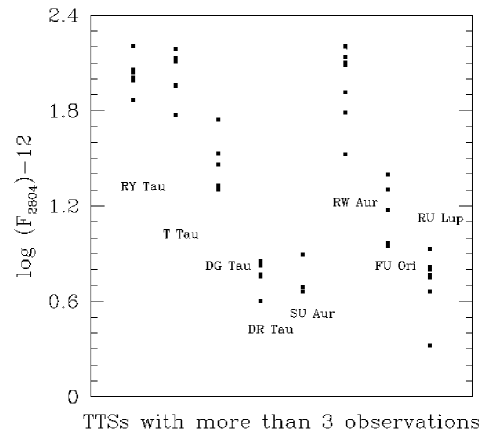
Figure 6: Mg II flux variability for the TTSs with multiple (more than three) good observations.

With this precaution in mind, we have compared the Mg II flux with other relevant tracers of the TTSs environment. We have selected for this purpose:

• The nearby UV continuum dominated by the Balmer continuum radiation produced in the accretion flow (see e.g. Ingleby et al., 2013) measured in the window [2730-2780] Å.

• The C IV emission produced by hot plasmas in the accretion flow (Ardila et al., 2013).

• The He II emission from the transition region and/or the accretion shock (Gómez de Castro, 2013b).

• The (P(2) 0-4) 1338.63 Å emission from H₂ produced by the molecular gas in the accretion disc around the TTSs (France et al., 2012). This radiation is, in turn, pumped by photons at 1217.205 Å  in the red wing of the Ly-$\alpha$ line (see e.g. Herczeg et al., 2002).

As shown in Fig. 7 and in Table 6, there is a correlation between the Mg II and the C IV flux, as well as with the He II flux; there is, however, no correlation with the UV continuum, nor with the H₂.

Table 6: Details about the flux-flux correlation between the Mg II and other spectral tracers.

	No. of	Pearson Cor.	$p{\rm-value}=p^{(*)}$
	obs.	Coeff.
$\frac{F(MgII)}{F_{bol}}$ vs $\frac{F(UVCont.)}{F_{bol}}$	41	0.34	0.03
$\frac{F(MgII)}{F_{bol}}$ vs $\frac{F(CIV)}{F_{bol}}$	25	0.68	0.0002
$\frac{F(MgII)}{F_{bol}}$ vs $\frac{F(HeII)}{F_{bol}}$	28	0.575	0.002
$\frac{F(MgII)}{F_{bol}}$ vs $\frac{F(H_{2})}{F_{bol}}$	14	0.29	0.313

$(*)$ $p{\rm-value}=p$ means that, for a random population there is

$100\cdot p$ % probability that the cross-correlation coefficient

will be $r$ or better. We are assuming that the correlation coefficient

is statistically significant if the $p{\rm-value}$ is lower than 5%.

Figure 7: Mg II flux normalized to the bolometric flux of the sources against other relevant UV tracers (see text). Triangles represent WTTSs.

4.2 Characterization of the Mg II profiles: asymmetry, dispersion and broadening

For this purpose we worked only with the highest S/N profiles for any given source. All measurements were carried out on the 2804 Å line. We measured:

• The asymmetry of the profile defined as $A=(F_{r})/(F_{r}+F_{b})$, i.e. $A=0.5$ for a symmetric line, $A=1$ for a fully absorbed blue wing and $A>1$ if the absorption goes below the continuum level.

• The second statistical moment: dispersion ($\sigma$).

• The width of the profile at the base of the line $\Delta V$. The red and blue edge velocities of the profile, $V_{r}$ and $V_{b}$, are defined as the point where the profile meets the continuum plus 1$\sigma$ at the red and blue edges of the profile respectively (see Fig. 8).

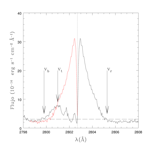
Figure 8: Example profile showing how we measured the terminal velocity of the wind ($V_{term}$) and the blue and red edge velocity of the profile ($V_{b}$ and $V_{r}$, respectively).

Red and blue fluxes ($F_{r}$ and $F_{b}$) were measured, as is explained in Section 4.1, from the center of the line to $V_{r}$ and from $V_{b}$ to line center, respectively. The dispersion was calculated from the gaussian fitting to the red wing symmetric profile at 2804 Å, i.e. it is the second statistical moment of the gaussian fit of an artificial and symmetric profile as shown in Fig. 9. Note that the moment is calculated avoiding the core of the line and the blue wing, where the circumstellar and the wind absorption components reside. For the stars AK Sco, CY Tau, UX Tau and HBC 388 the dispersion was calculated from the gaussian fit to the blue wing because the red wing is more absorbed than the blue wing.

Figure 9: The figure illustrates the artificial profile (solid line) used to measure the statistical moment of the profile plot over the observed line profile (dotted line) and the gaussian fit to the artificial profile (dashed line) for RU Lup.

4.2.1 Flux-dispersion relation

WTTSs have small dispersions and CTTSs have larger dispersions. The smallest dispersion is $\sigma\simeq 16$ km s^-1 for TWA 7. The highest dispersions are observed for RW Aur, CV Cha and AK Sco with $\sigma\simeq 171$, $169$ and $165$ km s^-1, respectively. For most of WTTSs, the line broadening is likely due to the plasma thermal velocity ($v_{th}\sim 12$ km s^-1 for a $T_{e}\simeq 10^{4}$ K) and the stellar rotation ($v{\rm sin}(i)\simeq 20$ km s^-1). However, line broadening for CTTSs is $50\la\sigma\la 170$ km $s^{-1}$, i.e. larger than the corresponding thermal and rotational velocities. There is a trend between the Mg II flux and the line broadening. Fig. 10 (bottom panel) shows the relation between the Mg II surface flux and the dispersion with $r=0.66$ and a $p{\rm-value}=1.55\times 10^{-6}$. The correlation does not improve when the profiles are corrected by the wind absorption taking into account the line asymmetry ($r=0.65$ and a $p{\rm-value}=2.86\times 10^{-6}$), as shown in the top panel of Fig. 10.

Figure 10: Flux-dispersion relation. Triangles represent WTTSs. Top: Mg II flux corrected by effect of the line asymmetry. Bottom: Mg II flux corrected by effect of luminosity.

4.2.2 Dispersion-rotation relation

To further explore the connection between stellar rotation $v{\rm sin}(i)$ and line broadening, we plotted them in Fig. 11, confirming that the line broadening is not associated with stellar rotation.

Figure 11: Dispersion as a function of $v{\rm sin}(i)$. Triangles represent WTTSs.

4.2.3 Flux-asymmetry relation

There is not a correlation between Mg II flux and profile asymmetry. This lack of trend is expected if the asymmetry is associated with the orientation of the outflow with respect to the line of sight (see Fig. 12). WTTSs and CTTSs have similar asymmetry values distributed in a broad range, from $\sim 0.4$ (for AK Sco and HBC 388, stars with nearly symmetric profiles) to $\sim 1$ (for T Tau, with absorbed blue wing).

Figure 12: Relation between the normalized 2804 Å line asymmetry and 2804 Å line flux. Triangles represent WTTSs.

4.2.4 Asymmetry-dispersion-inclination relation

Fig. 13 shows the dispersion ($\sigma$) as a function of the line asymmetry ($A$), where no significant correlation was found.

Figure 13: Relation between dispersion and asymmetry of TTSs in the sample. Triangles represent WTTSs.

A relation between asymmetry and inclination (see Table 2) is expected if the asymmetry is associated with the orientation of the outflow with respect to the line of sight. However, Fig. 14 does not show this connection. The lack of correlation could be due to the uncertainties in inclination measurements. Also, if the outflow is perpendicular to the disc, inclination values derived from stellar $v\sin i$ measurements are not reliable.

Figure 14: Inclination as a function of asymmetry. Triangles represent WTTSs. .

Note that if Mg II radiation is dominated by the outflow, there should be a correlation between inclination and dispersion or flux that it is not observed.

4.2.5 Relation between $\Delta V$, $V_{r}$, $V_{b}$ and dispersion

As shown in Fig. 15 (top panel), the dispersion and the width measured at the base of the line are correlated ($r=0.9$ and a $p{\rm-value}=0.00$). In addition the velocities in the blue and red edges of the profile ($V_{b}$ and $V_{r}$, respectively) correlate with the dispersion. This indicates that both line core and the wings radiation are generated by the same phenomenon, i.e. in the majority of sources the flux in the wings is not dominated by extended features such as unresolved jets. Otherwise we would observe more extended wings and we would not see this correlation.

Figure 15: Velocities at the profile edge compared with the dispersion. Triangles represent WTTSs.

The correlation in middle panel of Fig. 15 between dispersion and $V_{r}$ is better ($r=0.92$ and a $p{\rm-value}=0.00$) than with $V_{b}$ ($r=-0.75$ and a $p{\rm-value}=0.00$) in bottom panel, because of the larger uncertainties in $V_{b}$ due to the absorption by the wind. Moreover, $V_{r}-V_{b}$ correlates with the flux, as we can see in Fig. 16 ($r=0.7$ and a $p{\rm-value}=1.19\times 10^{-7}$).

Figure 16: Relation between Mg II flux and the Mg II lines width. Triangles represent WTTSs.

4.3 Terminal velocity wind

Measuring the terminal velocity of the outflow ($V_{term}$) from the Mg II profiles is challenging in TTSs. There are some sources like DE Tau or T Tau that display sharp blue edges and terminal velocities can be measured accurately. These stars are marked in Table 3 with an asterisk. However, for most of the sources, the blue edge is not sharp (see e.g., CV Cha, FU Ori or DR Tau). Moreover, the wind absorption is not observed against the continuum, as in the standard P-Cygni profiles produced by the outflows from massive stars (see for instance Talavera & Gomez de Castro, 1987). The wind absorption is observed against the broad Mg II emission from the accretion engine. We have hypothesized that the red wing truly represents the underlying symmetric profile and measured the terminal velocity as the point where the absorption meets the continuum plus $\sigma$ (the standard deviation of the continuum), as shown in Fig. 8. The measurements were done independently by the two co-authors and then compared, finding an agreement better than 10 km s^-1 between both sets of measurements (see Table 3, for the results). For figures, $V_{term}$ corresponding to the best observation (best S/N) is considered.

Note that the wind structure is very different for the various sources of the sample. In some cases, it just absorbs the blue wing of a rather narrow profile (this is typically observed in WTTSs). In other sources, there are double absorption bumps (see e.g. DN Tau or GM Aur profiles). Unfortunately, there are not time series following the evolution of these components. As shown in the Appendix A, the wind absorption (and the profile) do change in the stars for which several observations are available.

In the top left panel of Fig. 17, the terminal velocity $V_{term}$ it is shown to depend on the profile dispersion with $r=-0.8$ and a $p{\rm-value}=0.0000$ (for stars with $V_{term}>0$ km s^-1). One may naively think that this correlation is produced by the measurement procedure since the absorption is measured against the broad blue-wards shifted emission. However, a careful inspection of Fig. 1 shows that $V_{term}$ is controlled by the sharp blue-edge of the wind absorption. We did not find a significant correlation between the terminal velocity neither with profile asymmetry nor with flux (see top right and bottom panel of Fig. 17).

Figure 17: Terminal velocity as a function of dispersion, asymmetry and flux. Triangles represent WTTSs.

4.4 Profile variability

Repeated observations are available for 17 stars but significant profile variations are observed only in some of them, namely, BP Tau, RY Tau, T Tau, DF Tau, DG Tau, DR Tau, RW Aur, TW Hya and RU Lup (see Table 3 and Appendix A). In most of them, the variations are associated with the absorption components in the blue wing of the profile and they are more noticeable in profiles displaying several absorption components than in those displaying broad, saturated absorption components; blue wing absorptions seem to be associated to variable or episodic ejection. The terminal velocity of the flow varies only in few sources: DR Tau, DS Tau, FU Or, RU Lup, RY Tau, SU Aur and T Tau.

5 Constraints to the physics of TTS outflows

This work provides some important constraints to the physics of the TTSs outflows. The first constraint derives from the comparison between the Ly-$\alpha$ and Mg II profiles. As shown in Fig. 1, the blueshifted absorption produced by the wind, the sharp blue-edge indicating that the terminal velocity is reached, the variable discrete absorption components observed in some sources (e.g., SU Aur and BP Tau) are observed in the Mg II lines and remain undetectable in the Ly-$\alpha$ profile, even in the unabsorbed wings. This indicates that the wind is warm ($\log{\rm T}_{\rm e}\simeq 4-4.3$) and keeps a rather constant temperature in the acceleration region. Note that the absorption ranges from small velocities to typical protostellar jets speeds. This temperature regime is cooler than the detected in the semiforbidden Si III], C III] transitions (Gómez de Castro & Verdugo, 2001, 2007).

The Mg II profiles show that the wind covers a broad range of projected velocities along the line of sight. This, in turn, indicates that either the wind is kept isothermal while expanding radially or the outflow geometry is not radial, even at the base of the wind. Since large scale outflows from TTSs are collimated, this observation sets-up scales of several stellar radii for wind collimation.

The detection of DACs in some sources suggests that mass ejection is episodic even at small scales. This is consistent with the observations of knots in optical jets. One may wonder whether the broad absorptions are caused by the blending of many DACs, at least in some sources. Note that the current framework for modelling of mass ejection in TTSs includes episodic phenomenon produced by reconnection events in the magnetospheric star-disc boundary layer, see e.g. von Rekowski & Brandenburg (2004, 2006), earlier works by Goodson et al. (1997, 1999); Goodson & Winglee (1999) or later works by Romanova et al. (2012). However, Mg II observations show smooth absorption profiles. Henceforth, either the environmental conditions in early phases are such that the density in the current layer makes it prone to more frequent reconnection (for instance the higher density) producing a blending of broad DACs showing as a smooth absorption profile or Mg II is tracing another wind component, more likely the disc wind. Some constraints to the physics of TTS outflows are:

Evidence of latitude-dependent outflow on stellar scales from the profile asymmetry. A larger asymmetry is expected for pole-on systems, since the wind produces a larger blue wing absorption in these systems. However, we did not find a connection between inclination and profile asymmetries. This lack of correlation could be due to the uncertainties of the inclinations. In addition, we studied the possible relations among asymmetry and other magnitudes, such as flux, dispersion and terminal velocity of the wind, but we did not find any significant correlation.

Relation between Mg II emission and wind/outflow. The processes responsible for line broadening are related with Mg II flux emission (see Fig.10). Fig. 17 (top left panel) shows a connection between dispersion and terminal velocity of the wind. However, it is unclear from the data whether this connection is direct, i.e., the outflow contributes significantly to the Mg II line emission, or indirect through the well reported connection between accretion rate and wind signatures (see, for instance, Cabrit et al., 1990; Gomez de Castro & Pudritz, 1993). In a recent work (López-Martínez & Gómez de Castro, 2014), we have shown that the radiation in single ionized forbidden lines such as C II], Fe II] and Si II] is dominated by the extended stellar magnetosphere and the accretion flow. These lines trace a thermal regime similar to that traced by the Mg II lines, thus though we might expect a contribution from the wind to the Mg II flux, it seems accreting plasma dominates the line radiation. Therefore, the correlation we report between the dispersion and the $v_{term}$ is most likely indirect, both observables depend on the accretion rate.

The role of the gravitational field in mass ejection. To study where wind launching occurs, we have examined the relation between terminal velocity of the flow and escape velocity ($V_{esc}$) from the stellar surface (see Fig 18). Escape velocity was computed as $v_{esc}=\sqrt{2GM_{*}/R_{*}}$ where $R_{*}=\sqrt{L_{*}/(4\pi\sigma T_{eff}^{4})}$ using $L_{*}$, M_∗ and T_eff from Table 2. The escape velocities from stellar surface are larger than the terminal velocities of wind measured in the profiles. All measurements satisfy $V_{esc}<V_{term}$ going from the small $V_{esc}=-150$ km/s to the high $V_{esc}=-350$ km/s values. This suggests there is some scaling law between escape and projected terminal velocity. Note that our $V_{term}$ values correspond to the projection of the terminal velocity in the line of sight and thus, it is affected by inclination effects.

Figure 18: Escape velocity ($v_{esc}$) from stellar surface as a function of the Terminal velocity ($v_{term}$). Dashed line indicates where $v_{term}=v_{esc}$. Triangles represent WTTSs.

6 Relation between the Mg II radiation and magnetospheric emission

The temperature of the TTSs magnetospheres is expected to be rather cool, about some few thousands Kelvin (Romanova et al., 2012; Kulkarni & Romanova, 2013). Hence, we might expect that an uncertain fraction of the line flux is produced in the magnetosphere and that magnetospheric rotation and turbulence produce the line broadening.

In this context, it is confusing the lack of a strong correlation between accretion rate and Mg II flux, see the bottom panel of Fig. 19 ($r=0.5$ and $p{\rm-value}=0.002$) and also Fig. 7 for the correlation with the UV continuum radiation. Correcting the Mg II from the wind absorption does not improve significantly the trend; $r=0.54$ and a $p{\rm-value}=0.0007$ (see top panel of Fig. 19). Hence, radiation from the accretion flow does not seem to dominate the bulk of the Mg II radiation. We note that accretion rates used in this work come form other authors measurements (mainly from Ingleby et al., 2013) and thus Mg II and accretion rate measurements are not simultaneous. As shown in Fig. 6, fluxes can vary by a factor of 2 in accreting sources and this variability may affect to the reported lack of correlation.

Figure 19: Comparison between accretion rate ($M_{\sun}yr^{-1}$) and Mg II flux (2804 Å). Triangles represent WTTSs. Top: Mg II flux corrected by asymmetry and luminosity effects. Bottom: Mg II corrected by luminosity effect.

However, there seems to be a correlation between the line broadening and the accretion rate, as shown in Fig. 20 ($r=0.66$ and $p{\rm-value}=2.14\times 10^{-5}$).

Figure 20: Relation between the dispersion and the accretion rate ($M_{\sun}yr^{-1}$). Triangles represent WTTSs.

We searched a connection between the strength of the Mg II emission and the magnetospheric radius, that could provide some hints on the role of magnetospheric radiation on the dissipation of the angular momentum excess (see Gómez de Castro & Marcos-Arenal, 2012, for a recent study).
The size of the magnetosphere is set by the balance between the toroidal component of the stellar magnetic flux and the angular momentum of the infalling matter (Ghosh & Lamb, 1979):

$$R_{\rm mag}=\left(\frac{\gamma^{2}\mu^{4}}{GM_{*}M_{acc}^{2}}\right)^{1/7}$$

with $\mu=B_{*}R_{*}^{3}$, the equatorial magnetic moment of the star, $\gamma=(B_{t}/B_{p})(\Delta r/r)\simeq 0.5-0.8$ (see Lamb, 1989), $M_{acc}$ is the accretion rate and $B_{*}$ is the surface magnetic field. The magnetospheric radius can be calculated for a small subset of the stars. Surface magnetic fields were measured for AA Tau, DE Tau, DK Tau, DN Tau, GM Aur, T Tau, CY Tau, BP Tau, DF Tau, DG Tau, TW Hya (see Johns-Krull, 2007) and CV Cha (Gregory et al., 2012). However, no significant relation was found between the radius in this way determined and the Mg II normalized flux (see Fig. 21). Thus, not conclusive results can be inferred from the plot.

Figure 21: Relation between normalized 2804 Å line flux and magnetospheric radius ($R_{mag}$).

7 Conclusions

The analysis of the TTS Mg II profiles has provided new insights on the behaviour of the wind engine, including the magnetosphere, the accretion flow and the outflow. The main conclusions that have been drawn from this work are:

1. There is a warm wind that at sub-AU scales absorbs the blue wing of the Mg II profile. Thus, these lines are an ideal tracer of the wind acceleration region.

2. We find a relation between the line broadening both with the terminal velocity and with the accretion rate. This result could be an evidence that the accretion drives the winds/outflows processes.

3. The profile broadening, as measured from the dispersion, correlates with the velocity at the edge of the wings ($V_{r}$, $V_{b}$)

4. A mild correlation is found between the Mg II flux and the accretion rate.

5. We find a connection between line broadening and Mg II flux. Both outflow and magnetospheric plasma contribute to the Mg II flux; however, separating both contributions is very complex and model-dependent, monitoring programs are needed for this type of work.

We would like to emphasize the current uncertainties in age and mass for PMS stars. This work shows the potentials of high resolution UV spectroscopy to study the wind engine in PMS stars. Dedicated monitoring programs would be fundamental to study the wind acceleration region, especially in sources such as RY Tau where variable discrete components have been detected.

Appendix A Log of the Ly-$\alpha$ observations and variability of the Mg II profiles

In this section we include the log of the Ly-$\alpha$ observations (see Table 7). Also, the figures showing the variability of the Mg II profiles in the TTSs (see Fig. that is available online) are shown. Only observations with good enough S/N are compared.

Table 7: Telescope/instrument details for the Ly-$\alpha$ observations of the stars in the sample. The full table is available online as Supporting Information.

Star	Instrument	Obs. Date	Data set	Res.	Exposure
		(yy-mm-dd)	Id.	power	Time (s)
AA Tau	HST/COS	11-01-06	LB6B07040	19000	2844.3
	HST/COS	11-01-07	LB6B07050	18000	2844.4
AK Sco	HST/STIS	10-08-21	OB6B21040	45800	2917.2
BP Tau	HST/COS	11-09-09	LBGJ01050	18000	1150.2
	HST/COS	11-09-09	LBGJ01060	18000	1190.2
	HST/COS	11-09-09	LBGJ01070	19000	1397.2
	HST/COS	11-09-09	LBGJ01080	19000	1396.2
CS Cha	HST/COS	11-06-01	LB6B16010	18000	1177.9
	HST/COS	11-06-01	LB6B16020	19000	1177.9
CV Cha	HST/STIS	13-11-04	OB6B18030	45800	3265.2

References

- Andersen et al. (1989) Andersen, J., Lindgren, H., Hazen, M. L., & Mayor, M. 1989, A&A, 219, 142
- Ardila & Basri (2000) Ardila, D. R., & Basri, G. 2000, ApJ, 539, 834
- Ardila et al. (2002) Ardila, D. R., Basri, G., Walter, F. M., Valenti, J. A., & Johns-Krull, C. M. 2002, ApJ, 566, 1100
- Ardila et al. (2002) Ardila, D. R., Basri, G., Walter, F. M., Valenti, J. A., & Johns-Krull, C. M. 2002, ApJ, 567, 1013
- Ardila et al. (2013) Ardila, D. R., Herczeg, G. J., Gregory, S. G., et al. 2013, ApJS, 207, 1
- Ayres (2010) Ayres, T. R. 2010, ApJS, 187, 149
- Azevedo et al. (2006) Azevedo, R., Calvet, N., Hartmann, L., et al. 2006, A&A, 456, 225
- Basri & Bertout (1989) Basri, G., & Bertout, C. 1989, ApJ, 341, 340
- Berger et al. (2011) Berger, J.-P., Monnier, J. D., Millan-Gabet, R., et al. 2011, A&A, 529, L1
- Bertout et al. (1988) Bertout, C., Basri, G., & Bouvier, J. 1988, ApJ, 330, 350
- Bertout et al. (1999) Bertout, C., Robichon, N., & Arenou, F. 1999, A&A, 352, 574
- Bertout et al. (2007) Bertout, C., Siess, L., & Cabrit, S. 2007, A&A, 473, L21
- Bouvier (1990) Bouvier, J. 1990, AJ, 99, 946
- Bouvier et al. (1993) Bouvier, J., Cabrit, S., Fernandez, M., Martin, E. L., & Matthews, J. M. 1993, A&A, 272, 176
- Bouvier et al. (1995) Bouvier, J., Covino, E., Kovo, O., et al. 1995, A&A, 299, 89
- Cabrit et al. (1990) Cabrit, S., Edwards, S., Strom, S. E., & Strom, K. M. 1990, ApJ, 354, 687
- Calvet et al. (1985) Calvet, N., Basri, G., Imhoff, C. L., & Giampapa, M. S. 1985, ApJ, 293, 575
- Calvet & Gullbring (1998) Calvet, N., & Gullbring, E. 1998, ApJ, 509, 802
- Calvet et al. (2000) Calvet, N., Hartmann, L., & Strom, S. E. 2000, Protostars and Planets IV, 377
- Calvet et al. (2004) Calvet, N., Muzerolle, J., Briceño, C., et al. 2004, AJ, 128, 1294
- Camenzind (1990) Camenzind, M. 1990, Reviews in Modern Astronomy, 3, 234
- Canuto & Mazzitelli (1991) Canuto, V. M., & Mazzitelli, I. 1991, ApJ, 370, 295
- Cassatella et al. (2000) Cassatella, A., Altamore, A., González-Riestra, R., et al. 2000, APSS, 141, 331
- Catala et al. (1986) Catala, C., Czarny, J., Felenbok, P., & Praderie, F. 1986, A&A, 154, 103
- Clarke & Bouvier (2000) Clarke, C. J., & Bouvier, J. 2000, MNRAS, 319, 457
- Coffey et al. (2008) Coffey, D., Bacciotti, F., & Podio, L. 2008, ApJ, 689, 1112
- Coffey et al. (2007) Coffey, D., Bacciotti, F., Ray, T. P., Eislöffel, J., & Woitas, J. 2007, ApJ, 663, 350
- Coffey et al. (2012) Coffey, D., Rigliaco, E., Bacciotti, F., Ray, T. P., & Eislöffel, J. 2012, ApJ, 749, 139
- Correia et al. (2006) Correia, S., Zinnecker, H., Ratzka, T., & Sterzik, M. F. 2006, A&A, 459, 909
- D’Antona & Mazzitelli (1997) D’Antona, F., & Mazzitelli, I. 1997, MEMSAI, 68, 807
- da Silva et al. (2009) da Silva, L., Torres, C. A. O., de La Reza, R., et al. 2009, A&A, 508, 833
- Donati et al. (2012) Donati, J.-F., Gregory, S. G., Alencar, S. H. P., et al. 2012, MNRAS, 425, 2948
- Donati et al. (2007) Donati, J.-F., Jardine, M. M., Gregory, S. G., et al. 2007, MNRAS, 380, 1297
- Donati et al. (2008) Donati, J.-F., Jardine, M. M., Gregory, S. G., et al. 2008, MNRAS, 386, 1234
- France et al. (2012) France, K., Schindhelm, E., Herczeg, G. J., et al. 2012, ApJ, 756, 171
- Furlan et al. (2006) Furlan, E., Hartmann, L., Calvet, N., et al. 2006, ApJs, 165, 568
- Ghosh & Lamb (1979) Ghosh, P., & Lamb, F. K. 1979, ApJ, 232, 259
- Giampapa et al. (1981) Giampapa, M. S., Calvet, N., Imhoff, C. L., & Kuhi, L. V. 1981, ApJ, 251, 113
- Gómez de Castro (1998) Gómez de Castro, A. I. 1998, Ultraviolet Astrophysics Beyond the IUE Final Archive, 413, 59
- Gómez de Castro (2009a) Gómez de Castro, A. I. 2009a, APSS, 320, 97
- Gómez de Castro (2009b) Gómez de Castro, A. I. 2009b, ApJl, 698, L108
- Gómez de Castro (2013a) Gómez de Castro, A. I. 2013a, Planets, Stars and Stellar Systems. Volume 4: Stellar Structure and Evolution, 279
- Gómez de Castro (2013b) Gómez de Castro, A. I. 2013b, ApJ, 775, 131
- Gómez de Castro & Fernández (1996) Gómez de Castro, A. I., & Fernández, M. 1996, MNRAS, 283, 55
- Gómez de Castro & Franqueira (1997) Gomez de Castro, A. I., & Franqueira, M. 1997, ApJ, 482, 465
- Gomez de Castro & Lamzin (1999) Gomez de Castro, A. I., & Lamzin, S. A. 1999, MNRAS, 304, L41
- Gómez de Castro et al. (2013c) Gómez de Castro, A. I., López-Santiago, J., Talavera, A., Sytov, A. Y., & Bisikalo, D. 2013c, ApJ, 766, 62
- Gómez de Castro & Marcos-Arenal (2012) Gómez de Castro, A. I., & Marcos-Arenal, P. 2012, ApJ, 749, 190
- Gomez de Castro & Pudritz (1993) Gomez de Castro, A. I., & Pudritz, R. E. 1993, ApJ, 409, 748
- Gómez de Castro & Verdugo (2001) Gómez de Castro, A. I., & Verdugo, E. 2001, ApJ, 548, 976
- Gómez de Castro & Verdugo (2003) Gómez de Castro, A. I., & Verdugo, E. 2003, ApJ, 597, 443
- Gómez de Castro & Verdugo (2007) Gómez de Castro, A. I., & Verdugo, E. 2007, ApJl, 654, L91
- González-Riestra et al. (2000) González-Riestra, R., Cassatella, A., Solano, E., Altamore, A., & Wamsteker, W. 2000, A&AS, 141, 343
- Goodson et al. (1999) Goodson, A. P., Böhm, K.-H., & Winglee, R. M. 1999, ApJ, 524, 142
- Goodson & Winglee (1999) Goodson, A. P., & Winglee, R. M. 1999, ApJ, 524, 159
- Goodson et al. (1997) Goodson, A. P., Winglee, R. M., & Boehm, K.-H. 1997, ApJ, 489, 199
- Gregory et al. (2012) Gregory, S. G., Donati, J.-F., Morin, J., et al. 2012, ApJ, 755, 97
- Güdel et al. (2008) Güdel, M., Skinner, S. L., Audard, M., Briggs, K. R., & Cabrit, S. 2008, A&A, 478, 797
- Gullbring et al. (2000) Gullbring, E., Calvet, N., Muzerolle, J., & Hartmann, L. 2000, ApJ, 544, 927
- Gullbring et al. (1998) Gullbring, E., Hartmann, L., Briceno, C., & Calvet, N. 1998, ApJ, 492, 323
- Hartigan et al. (1995) Hartigan, P., Edwards, S., & Ghandour, L. 1995, ApJ, 452, 736
- Hartmann et al. (1990) Hartmann, L., Avrett, E. H., Loeser, R., & Calvet, N. 1990, ApJ, 349, 168
- Hartmann et al. (1998) Hartmann, L., Calvet, N., Gullbring, E., & D’Alessio, P. 1998, ApJ, 495, 385
- Hartmann et al. (1994) Hartmann, L., Hewett, R., & Calvet, N. 1994, ApJ, 426, 669
- Hartmann et al. (1986) Hartmann, L., Hewett, R., Stahler, S., & Mathieu, R. D. 1986, ApJ, 309, 275
- Hartmann et al. (2004) Hartmann, L., Hinkle, K., & Calvet, N. 2004, ApJ, 609, 906
- Herbst et al. (1996) Herbst, T. M., Beckwith, S. V. W., Glindemann, A., et al. 1996, AJ, 111, 2403
- Herczeg & Hillenbrand (2008) Herczeg, G. J., & Hillenbrand, L. A. 2008, ApJ, 681, 594
- Herczeg et al. (2002) Herczeg, G. J., Linsky, J. L., Valenti, J. A., Johns-Krull, C. M., & Wood, B. E. 2002, ApJ, 572, 310
- Herczeg et al. (2006) Herczeg, G. J., Linsky, J. L., Walter, F. M., Gahm, G. F., & Johns-Krull, C. M. 2006, ApJs, 165, 256
- Herczeg et al. (2004) Herczeg, G. J., Wood, B. E., Linsky, J. L., Valenti, J. A., & Johns-Krull, C. M. 2004, ApJ, 607, 369
- Hughes et al. (1994) Hughes, J., Hartigan, P., Krautter, J., & Kelemen, J. 1994, AJ, 108, 1071
- Hussain et al. (2009) Hussain, G. A. J., Collier Cameron, A., Jardine, M. M., et al. 2009, MNRAS, 398, 189
- Imhoff & Giampapa (1980) Imhoff, C. L., & Giampapa, M. S. 1980, ApJl, 239, L115
- Ingleby et al. (2011) Ingleby, L., Calvet, N., Bergin, E., et al. 2011, ApJ, 743, 105
- Ingleby et al. (2013) Ingleby, L., Calvet, N., Herczeg, G., et al. 2013, ApJ, 767, 112
- Jayawardhana et al. (2006) Jayawardhana, R., Coffey, J., Scholz, A., Brandeker, A., & van Kerkwijk, M. H. 2006, ApJ, 648, 1206
- Johns-Krull (2007) Johns-Krull, C. M. 2007, ApJ, 664, 975
- Johns-Krull et al. (2000) Johns-Krull, C. M., Valenti, J. A., & Linsky, J. L. 2000, ApJ, 539, 815
- Johns-Krull et al. (2004) Johns-Krull, C. M., Valenti, J. A., & Saar, S. H. 2004, ApJ, 617, 1204
- Koenigl (1991) Koenigl, A. 1991, ApJl, 370, L39
- Kulkarni & Romanova (2013) Kulkarni, A. K., & Romanova, M. M. 2013, MNRAS, 433, 3048
- Kundurthy et al. (2006) Kundurthy, P., Meyer, M. R., Robberto, M., Beckwith, S. V. W., & Herbst, T. 2006, AJ, 132, 2469
- Lamb (1989) Lamb, F. K. 1989, Annals of the New York Academy of Sciences, 571, 347
- Lamzin (2000) Lamzin, S. A. 2000, Astronomy Letters, 26, 225
- Lawson et al. (2001) Lawson, W. A., Crause, L. A., Mamajek, E. E., & Feigelson, E. D. 2001, MNRAS, 321, 57
- López-Martínez & Gómez de Castro (2014) López-Martínez, F., & Gómez de Castro, A. I. 2014, MNRAS, 442, 2951
- Mamajek et al. (2002) Mamajek, E. E., Meyer, M. R., & Liebert, J. 2002, AJ, 124, 1670
- Manoj et al. (2006) Manoj, P., Bhatt, H. C., Maheswar, G., & Muneer, S. 2006, ApJ, 653, 657
- Mathieu et al. (1991) Mathieu, R. D., Adams, F. C., & Latham, D. W. 1991, AJ, 101, 2184
- Muzerolle et al. (2003) Muzerolle, J., Calvet, N., Hartmann, L., & D’Alessio, P. 2003, ApJl, 597, L149
- Nguyen et al. (2012) Nguyen, D. C., Brandeker, A., van Kerkwijk, M. H., & Jayawardhana, R. 2012, ApJ, 745, 119
- Nguyen et al. (2009) Nguyen, D. C., Jayawardhana, R., van Kerkwijk, M. H., et al. 2009, ApJ, 695, 1648
- Nichols & Linsky (1996) Nichols, J. S., & Linsky, J. L. 1996, AJ, 111, 517
- Penston & Lago (1983) Penston, M. V., & Lago, M. T. V. T. 1983, MNRAS, 202, 77
- Petrov & Herbig (2008) Petrov, P. P., & Herbig, G. H. 2008, AJ, 136, 676
- Preibisch & Smith (1997) Preibisch, T., & Smith, M. D. 1997, A&A, 322, 825
- Romanova et al. (2012) Romanova, M. M., Ustyugova, G. V., Koldoba, A. V., & Lovelace, R. V. E. 2012, MNRAS, 421, 63
- Sacco et al. (2012) Sacco, G. G., Flaccomio, E., Pascucci, I., et al. 2012, ApJ, 747, 142
- Salyk et al. (2013) Salyk, C., Herczeg, G. J., Brown, J. M., et al. 2013, ApJ, 769, 21
- Sartoretti et al. (1998) Sartoretti, P., Brown, R. A., Latham, D. W., & Torres, G. 1998, A&A, 334, 592
- Schindhelm et al. (2012) Schindhelm, E.,France, K., Herczeg, G. J., et al. 2012, ApJ, 756, L23
- Siess et al. (2000) Siess, L., Dufour, E., & Forestini, M. 2000, A&A, 358, 593
- Simon et al. (1990) Simon, T., Vrba, F. J., & Herbst, W. 1990, AJ, 100, 1957
- Steffen et al. (2001) Steffen, A. T., Mathieu, R. D., Lattanzi, M. G., et al. 2001, AJ, 122, 997
- Stempels et al. (2007) Stempels, H. C., Gahm, G. F., & Petrov, P. P. 2007, A&A, 461, 253
- Sterzik et al. (1999) Sterzik, M. F., Alcalá, J. M., Covino, E., & Petr, M. G. 1999, A&A, 346, L41
- St-Onge & Bastien (2008) St-Onge, G., & Bastien, P. 2008, ApJ, 674, 1032
- Talavera & Gomez de Castro (1987) Talavera, A., & Gomez de Castro, A. I. 1987, A&A, 181, 300
- Unruh et al. (1998) Unruh, Y. C., Collier Cameron, A., & Guenther, E. 1998, MNRAS, 295, 781
- Valencic et al. (2004) Valencic, L. A., Clayton, G. C., & Gordon, K. D. 2004, ApJ, 616, 912
- von Rekowski & Brandenburg (2004) von Rekowski, B., & Brandenburg, A. 2004, A&A, 420, 17
- von Rekowski & Brandenburg (2006) von Rekowski, B., & Brandenburg, A. 2006, Astronomische Nachrichten, 327, 53
- Walter & Miner (2005) Walter, F. M., & Miner, J. 2005, 13th Cambridge Workshop on Cool Stars, Stellar Systems and the Sun, 560, 1021
- Wang et al. (2004) Wang, H., Apai, D., Henning, T., & Pascucci, I. 2004, ApJL, 601, L83
- White & Ghez (2001) White, R. J., & Ghez, A. M. 2001, ApJ, 556, 265
- Woitke et al. (2011) Woitke, P., Riaz, B., Duchêne, G., et al. 2011, A&A, 534, A44
- Yang et al. (2012) Yang, H., Herczeg, G. J., Linsky, J. L., et al. 2012, ApJ, 744, 121
- Yang et al. (2008) Yang, H., Johns-Krull, C. M., & Valenti, J. A. 2008, AJ, 136, 2286