Optical analogy to quantum computation based on classical fields modulated pseudorandom phase sequences

Abstract

We demonstrate that a tensor product structure and optical analogy of quantum entanglement can be obtained by introducing pseudorandom phase sequences into classical fields with two orthogonal modes. Using the classical analogy, we discuss efficient simulation of several typical quantum states, including product state, Bell states, GHZ state, and W state. By performing quadrature demodulation scheme, we propose a sequence permutation mechanism to simulate certain quantum states and a generalized gate array model to simulate quantum algorithm, such as Shor’s algorithm and Grover’s algorithm. The research on classical simulation of quantum states is important, for it not only enables potential beyond quantum computation, but also provides useful insights into fundamental concepts of quantum mechanics.

LABEL:FirstPage1

Introduction

It has been widely known that fast algorithm is not available for many famous computing problems according to classical computational complexity theory Garey . Quantum computation, however, enormously promotes computational efficiency with accumulation of computational complexity no faster than polynomial rate under linear increasement of input size by using several basic and purely physical features of quantum mechanics, such as coherent superposition, parallelism, entanglement, measurement collapse etc. Nielsen . The acceleratory ability of quantum computation is related to tensor product and quantum entanglement, of which the latter one is essential to realize quantum computation and quantum communication Jozsa ; Braunstein . Yet quantum algorithm is difficult to be realized for restrict of quantum system controllability, decoherence property and measurement randomness Knill ; Nielsen2 ; Browne ; Kok .

Recently, several researches have proposed a new concept of realization of classical entanglement based on classical optical fields by introducing a new freedom degree to realize tensor product in quantum entanglement Toppel . Further, Ref. Fu1 proposed that phase modulation by orthogonal pseudo-random sequence is able to simulate quantum entanglement effectively. In this scheme, these classical fields with an increased freedom degree not only realized tensor product structure but also simulated the nonlocal property of quantum entanglement by using property of orthogonal pseudo-random sequence like orthogonality, balance and closure. It is interesting that this simulation creates a Hilbert space of $n2^{n}$ dimensions which is larger than quantum mechanics. Different from quantum measurement involving collapse, these classical fields are measured in intensity by optical detectors directly.

The classical simulation of quantum systems, especially of quantum entanglement has been under investigation for a long time Cerf ; Massar ; Spreeuw . In addition to potential practical applications in quantum computation, research on classical simulation systems can help understand some fundamental concepts in quantum mechanics. However, it has been pointed out by several authors that classical simulation of quantum systems exhibits exponentially scaling of physical resources with the number of quantum particles Jozsa ; Spreeuw . In Ref. Spreeuw , an optical analogy of quantum systems is introduced, in which the number of light beams and optical components required grows exponentially with the number of qubits. In Ref. Vidal , a classical protocol to efficiently simulate any pure-state quantum computation is presented, yet the amount of entanglement involved is restricted. In Ref. Jozsa , it is elucidated that in classical theory, the state space of a composite system is the Cartesian product of subsystems, whereas in quantum theory it is the tensor product. This essential distinction between Cartesian and tensor products is precisely the phenomenon of quantum entanglement, and viewed as the origin of the limitation of classical simulation of quantum systems. Therefore it is of great significance in the classical simulations to realize tensor product Toppel ; Fu1 .

In wireless and optical communications, orthogonal pseudorandom sequences have been widely applied to Code Division Multiple Access (CDMA) communication technology as a way to distinguish different users Viterbi ; Peterson . A set of pseudorandom sequences is generated from a shift register guided by a Galois field GF($p$), which satisfies orthogonal, closure and balance properties Peterson . In Phase Shift Keying (PSK) communication systems PSK , pseudorandom sequences are used to modulate the phase of the electromagnetic/optical wave, where a pseudorandom sequence is mapped to a pseudorandom phase sequence (PPS) values in $\left\{0,2\pi/p,\cdots,2\pi\left(p-1\right)/p\right\}$. Guaranteed by the orthogonal property of the PPS, different electromagnetic/optical waves can transmit in one communication channel simultaneously without crosstalk, and can be easily distinguished by implementing a quadrature demodulation measurement Viterbi .

In this paper, we propose a new mechanism based on circular demodulation to realize simulation of certain quantum state represented by these classical optical fields. Besides, classical simulation of some other typical quantum states is discussed, including product state, Bell states, GHZ and W states. Furthermore, we propose a new scheme to simulate quantum computing by constructing certain quantum states based on an array of several mode control gates. Finally, we use this method to simulate Shor’s algorithm Shor ; Shor2 and Grover’s algorithm Grover .

The paper is organized as follows: In Section I, we introduce some preparing knowledge needed later in this paper. In Section II, the existence of the tensor product structure in our simulation is demonstrated and the classical simulation of several typical quantum states is analyzed. In Section III, a generalized gate array model to simulate quantum computation is proposed. Finally, we summarize our conclusions in Section IV.

I Preparing Knowledge

In this section, we introduce some notation and basic results needed later in this paper. We first introduce pseudorandom sequences and their properties. Then we discuss the similarities between classical optical fields and single-particle quantum states. Finally, we introduce the scheme of modulation and demodulation on classical optical fields with PPSs.

I.1 Pseudorandom sequences and their properties

As far as we know, orthogonal pseudorandom sequences have been widely applied to CDMA communication technology as a way to distinguish different users Viterbi ; Peterson . A set of pseudorandom sequences is generated from a shift register guided by a Galois Field GF($p$), which satisfies orthogonal, closure and balance properties. The orthogonal property ensures that sequences of the set are independent and distinguished each other with an excellent correlation property. The closure property ensures that any linear combination of the sequences remains in the same set. The balance property ensures that the occurrence rate of all non-zero-element in every sequence is equal, and the the number of zero-elements is exactly one less than the other elements.

One famous generator of pseudorandom sequences is Linear Feedback Shift Register (LFSR), which can produce a maximal period sequence, called m-sequence Peterson . We consider an m-sequence of period $N-1$ ($N=p^{s}$) generated by a primitive polynomial of degree $s$ over GF($p$). Since the correlation between different shifts of an m-sequence is almost zero, they can be used as different codes with their excellent correlation property. In this regard, the set of $N-1$ m-sequences of length $N-1$ can be obtained by cyclic shifting of a single m-sequence.

In this paper, we employ pseudorandom phase sequences (PPSs) with $2$-ary phase shift modulation, which is a well-known modulation format in wireless and optical communications, including PSK PSK . Different from Ref. Fu1 , we choose GF($2$) instead of GF($4$) because the correlation measurements for Bell inequality are not discussed in this paper. We first propose a scheme to generate a PPS set $\Xi=\left\{\lambda^{\left(0\right)},\lambda^{\left(1\right)},\ldots,\lambda^{\left(N-1\right)}\right\}$ over GF($2$) Peterson . $\lambda^{\left(0\right)}$ is an all-$0$ sequence and other sequences can be generated by using the method as follows:

(1) given a primitive polynomial of degree $s$ over GF($2$), a base sequence of a length $2^{s}-1$ is generated by using LFSR;

(2) other sequences are obtained by cyclic shifting of the base sequence;

(3) by adding a zero-element to the end of each sequence, the occurrence rates of all elements in all sequences are equal with each other;

(4) mapping the elements of the sequences to $\{0,\pi/2\}$: $0$ mapping $0$, $1$ mapping $\pi/2$.

Further, we define a map $f:\lambda\rightarrow e^{i\lambda}$ on the set of $\Xi$, and obtain a new sequence set $\Omega=\left\{\varphi^{\left(j\right)}\left|\varphi^{\left(j\right)}=e^{i\lambda^{\left(j\right)}},\right.j=0,\ldots,N-1\right\}$. In Fig. 1, we demonstrate the relationship between time slots, an m-sequence and phase sequence $\lambda^{\left(i\right)}$ with $N$ phase units $\lambda^{\left(i\right)}=[\lambda_{1}^{\left(i\right)},\lambda_{2}^{\left(i\right)},\cdots\lambda_{N}^{\left(i\right)}]$. For better understanding our scheme, the PPSs in the cases of modulating $7$ classical optical fields is illustrated below. Using the method mentioned in section I, an m-sequence of length $2^{3}-1$ is generated by a primitive polynomial of the lowest degree over $GF(2)$, which is $\left[\begin{array}[]{ccccccc}1&1&1&0&0&1&0\end{array}\right]$. Then we obtain a group that includes $8$ PPSs of length $8$: $\left\{\lambda^{\left(0\right)},\ldots,\lambda^{\left(7\right)}\right\}$, of which in exception to $\lambda^{\left(0\right)}$, all PPSs can be used to modulate classical optical fields to simulate quantum states of up to $7$ particles expect $\lambda^{\left(0\right)}$, for example,

$$\lambda^{\left(1\right)} = \left[\begin{array}[]{cccccccc}1&1&1&0&0&1&0&0\end{array}\right]\times\pi/2,$$ (2)

$$\lambda^{\left(2\right)} = \left[\begin{array}[]{cccccccc}1&1&0&0&1&0&1&0\end{array}\right]\times\pi/2,$$ (4)

$$\lambda^{\left(3\right)} = \left[\begin{array}[]{cccccccc}1&0&0&1&0&1&1&0\end{array}\right]\times\pi/2,$$ (6)

$$\lambda^{\left(4\right)} = \left[\begin{array}[]{cccccccc}0&0&1&0&1&1&1&0\end{array}\right]\times\pi/2,$$ (8)

$$\lambda^{\left(5\right)} = \left[\begin{array}[]{cccccccc}0&1&0&1&1&1&0&0\end{array}\right]\times\pi/2,$$ (10)

$$\lambda^{\left(6\right)} = \left[\begin{array}[]{cccccccc}1&0&1&1&1&0&0&0\end{array}\right]\times\pi/2,$$ (12)

$$\lambda^{\left(7\right)} = \left[\begin{array}[]{cccccccc}0&1&1&1&0&0&1&0\end{array}\right]\times\pi/2.$$ (14)

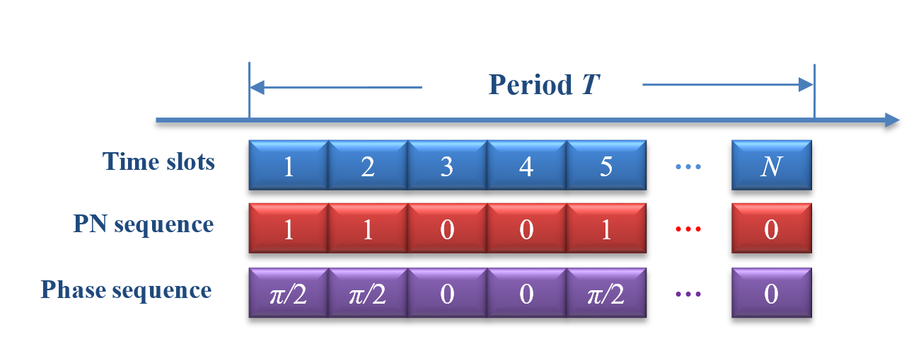
Figure 1: The time sequence relationship of the PPS is shown.

According to the properties of m-sequence, we can obtain following properties of the set $\Omega$, (1) the closure property: the product of any sequences remains in the same set; (2) the balance property: in exception to $\varphi^{\left(0\right)}$, any sequences of the set $\Omega$ satisfy

$$\sum\limits_{k=1}^{N}e^{i\theta}\varphi_{k}^{\left(j\right)}=\sum\limits_{k=1}^{N}e^{i\left(\lambda_{k}^{\left(j\right)}+\theta\right)}=0,\forall\theta\in\mathbb{R};$$ (15)

(3) the orthogonal property: any two sequences satisfy the following normalized correlation

$$E\left({\varphi^{\left(i\right)},\varphi^{\left(j\right)}}\right) = \frac{1}{N}\sum\limits_{k=1}^{N}{\varphi_{k}^{\left(i\right)}\varphi_{k}^{\left(j\right)\ast}}$$ (16)

$$= \left\{\begin{array}[]{cc}1,&i=j\\ 0,&i\neq j\end{array}\right..$$ (19)

In conclusion, the map $f$ corresponds to the modulation of PPSs of $\Omega$ on classical optical fields. According to the properties above, the classical optical fields modulated with different PPSs become independent and distinguishable.

I.2 Similarities between classical optical field and single-particle quantum states

We note the similarities between Maxwell equation and Schrödinger equation. In fact, some properties of quantum information are wave properties, where the wave is not necessary to be a quantum wave Spreeuw . Analogous to quantum states, classical optical fields also obey a superposition principle, and can be transformed to any superposition state by unitary transformations. Those analogous properties made the simulation of quantum states using polarization or transverse modes of classical optical fields possible Fu ; dragoman ; Lee .

We first consider two orthogonal modes (polarization or transverse), as the classical simulation of quantum bits (qubits) $\left|0\right\rangle$ and $\left|1\right\rangle$ Spreeuw ; Fu .

$$\left|0\right\rangle=\left(\begin{array}[]{c}1\\ 0\end{array}\right),\left|1\right\rangle=\left(\begin{array}[]{c}0\\ 1\end{array}\right).$$ (20)

Thus, any quantum state of a single particle can be simulated by a corresponding classical mode superposition field, as follows

$$\left|\psi\right\rangle=\alpha\left|0\right\rangle+\beta\left|1\right\rangle,\left|\alpha\right|^{2}+\left|\beta\right|^{2}=1,\left(\alpha,\beta\in\mathbb{C}\right).$$ (21)

Obviously, all the mode superposition fields can span a Hilbert space, where we can perform unitary transformations to transform the mode state. For example, the unitary transformation $U\left(\chi,\theta\right)$ is defined

$$U\left(\chi,\theta\right)=e^{i\chi\left(\sigma_{x}\cos\theta+\sigma_{y}\sin\theta\right)}=\left(\begin{array}[]{cc}\cos\chi&-ie^{i\theta}\sin\chi\\ ie^{-i\theta}\sin\chi&\cos\chi\end{array}\right),$$ (22)

where $\sigma_{x}$, $\sigma_{y}$ are Pauli matrices. The modes $\left|0\right\rangle$ and $\left|1\right\rangle$ can be transformed to mode superposition by using $U\left(\chi,\theta\right)$, respectively, as follows

$$U\left(\chi,\theta\right)\left|0\right\rangle = \cos\chi\left|0\right\rangle+ie^{i\theta}\sin\chi\left|1\right\rangle,$$ (23)

$$U\left(\chi,\theta\right)\left|1\right\rangle = \cos\chi\left|1\right\rangle-ie^{-i\theta}\sin\chi\left|0\right\rangle.$$

Now, we consider some devices with one input and two outputs, such as beam or mode splitters, which split one input field $\left|\psi_{in}\right\rangle=\alpha\left|0\right\rangle+\beta\left|1\right\rangle$ into two output fields $\left|\psi_{out}^{\left(a\right)}\right\rangle$ and $\left|\psi_{out}^{\left(b\right)}\right\rangle$. For the case of beam splitters, the output fields are $\left|\psi_{out}^{\left(a\right)}\right\rangle=C_{a}\left(\alpha\left|0\right\rangle+\beta e^{i\phi_{a}}\left|1\right\rangle\right)$ and $\left|\psi_{out}^{\left(b\right)}\right\rangle=C_{b}\left(\alpha\left|0\right\rangle+\beta e^{i\phi_{b}}\left|1\right\rangle\right)$ with an arbitrary power ratio $\left|C_{a}\right|^{2}:\left|C_{b}\right|^{2}$ between the output beams, where $\phi_{a,b}$ are the additional phases due to the splitter. For the case of mode splitters, the output fields are $\left|\psi_{out}^{\left(a\right)}\right\rangle=\alpha e^{i\phi_{a}}\left|0\right\rangle$ and $\left|\psi_{out}^{\left(b\right)}\right\rangle=\beta e^{i\phi_{b}}\left|1\right\rangle$, where $\phi_{a,b}$ are also the additional phases. Conversely, the devices can act as beam or mode combiners in which beams or modes from two inputs are combined into one output.

I.3 Modulation and demodulation on classical optical fields with pseudorandom phase sequences

We first consider the modulation process on a classical optical field with a PPS. Similar to PSK system, choosing a PPS $\lambda^{\left(i\right)}$ in the set of $\Xi$, the phase of the field can be modulated by a phase modulator (PM) that controlled by a pseudorandom number generator (PNG), the scheme is shown in Fig. 2. If the input is a single-mode field, it can be transformed to mode superposition by performing a unitary transformation after the modulation.

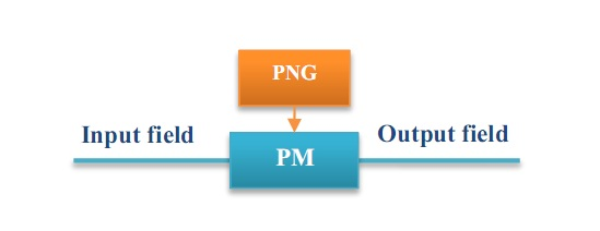
Figure 2: The PPS encoding scheme for one input field is shown, where PNG denotes the pseudorandom number generator and PM denotes the phase modulator.

Then we consider the quadrature demodulation process of a modulated classical optical field. Quadrature demodulation is a coherent detection process that allows the simultaneous measurement of conjugate quadrature components via homodyning the emerging beams with the input and reference fields by using a balanced beam splitting, where the reference field is modulated with a PPS $\lambda^{\left(r\right)}$. The differenced signals of two output detectors are then summed over $N$ and sampled to yield the decision variable. We can express the demodulation process in mathematical form

$$I\left(\lambda^{\left(i\right)},\lambda^{\left(r\right)}\right)=\frac{1}{N}\sum_{k=1}^{N}\cos\left(\lambda_{k}^{\left(i\right)}-\lambda_{k}^{\left(r\right)}\right)=\left\{\begin{array}[]{cc}1,&i=r\\ 0,&i\neq r\end{array}\right.,$$ (24)

where $\lambda_{k}^{\left(i\right)},\lambda_{k}^{\left(r\right)}$ are the PPSs of the input and reference fields respectively. The output decision variable is $1$ if and only if $\lambda_{k}^{\left(i\right)},\lambda_{k}^{\left(r\right)}$ are equal; otherwise the output decision variable is $0$. The results are guaranteed by the properties of PPSs. If the input is a single-mode field, the scheme shown in Fig. 3 is employed to perform quadrature demodulation. Otherwise the scheme shown in Fig. 4 is used, in which the input field $\left|\psi_{i}\right\rangle=e^{i\lambda^{\left(i\right)}}\left(\alpha_{i}\left|0\right\rangle+\beta_{i}\left|1\right\rangle\right)$ is first splitted into two fields $\alpha_{i}e^{i\lambda^{\left(i\right)}}\left|0\right\rangle$ and $\beta_{i}e^{i\lambda^{\left(i\right)}}\left|1\right\rangle$, and two coherent detection processes are then performed on the two fields respectively. Noteworthily, the modes of the reference fields must be consistent with the two output fields. Thus there are two output decision variables $\tilde{\alpha}$ and $\tilde{\beta}$, which correspond to the modes $\left|0\right\rangle$ and $\left|1\right\rangle$, respectively. We define $\left(\tilde{\alpha},\tilde{\beta}\right)$ as a mode status that displays not only existence of mode also phases due to the polarity of signals. Besides the quadrature demodulation, we can also easily measure the amplitudes of each modes $\left|\alpha_{i}\right|,\left|\beta_{i}\right|$ after mode spitting in the scheme. However, we will not deal with normalization of superposition coefficients $\alpha$ and $\beta$ in our scheme, because the amplitudes of each modes are not important.

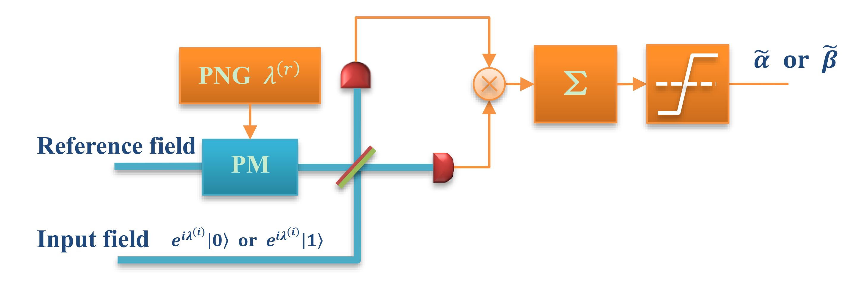
Figure 3: The PPS quadrature demodulation scheme for one input field with single mode $e^{i\lambda^{\left(i\right)}}\left|0\right\rangle$ or $e^{i\lambda^{\left(i\right)}}\left|1\right\rangle$ is shown.

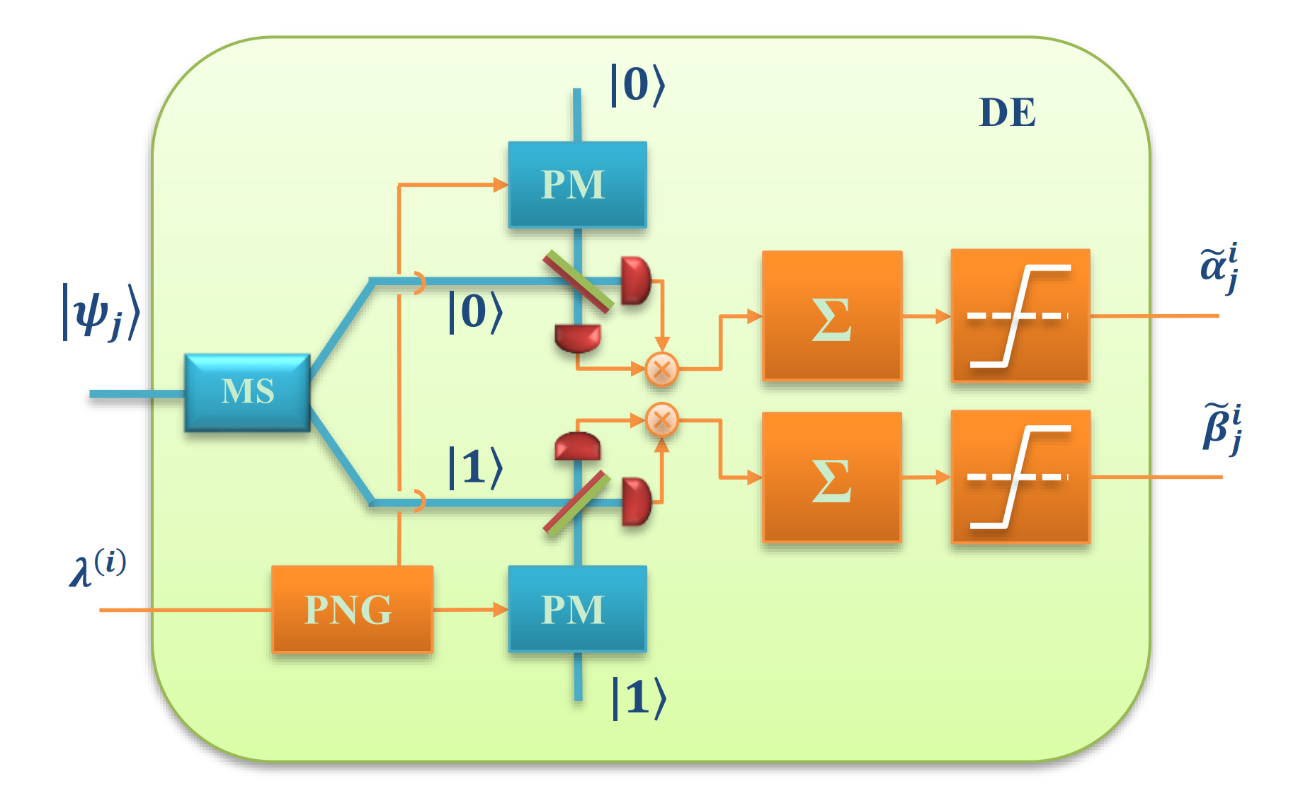
Figure 4: The PPS quadrature demodulation scheme for one field with two orthogonal modes is shown, where the blue block MS denote the mode splitter.

II Simulation of multiparticle quantum states

We discuss simulation of multiparticle quantum states using classical optical fields modulated with PPSs in this section. We first demonstrate that $n$ classical optical fields modulated with $n$ different PPSs can constitute a similar $n2^{n}$-dimensional Hilbert space that contains a tensor product structure Fu1 . Besides, by performing quadrature demodulation scheme, we can obtain the mode status matrix of the simulating classical optical fields, based on which we propose a sequence permutation mechanism to simulate the quantum states. Classical simulations of some typical quantum states are then discussed, including product state, Bell states, GHZ state and W state.

II.1 Classical optical fields modulated with pseudorandom phase sequences and their tensor product structure

For convenience, here we consider two classical optical fields modulated with PPSs and their tensor product structure. Chosen any two PPSs of $\lambda^{\left(a\right)}$ and $\lambda^{\left(b\right)}$ from the set $\Xi$, any two fields modulated with the PPSs can be expressed as follows,

$$\left|\psi_{a}\right\rangle = e^{i\lambda^{\left(a\right)}}\left(\alpha_{a}\left|0\right\rangle+\beta_{a}\left|1\right\rangle\right),$$ (25)

$$\left|\psi_{b}\right\rangle = e^{i\lambda^{\left(b\right)}}\left(\alpha_{b}\left|0\right\rangle+\beta_{b}\left|1\right\rangle\right).$$

We define the inner product of two fields $\left|\psi_{a}\right\rangle$ and $\left|\psi_{b}\right\rangle$ as follows,

$$\left\langle\psi_{a}|\psi_{b}\right\rangle=\frac{1}{N}\sum\limits_{k=1}^{N}e^{i\left(\lambda_{k}^{\left(b\right)}-\lambda_{k}^{\left(a\right)}\right)}\left(\alpha_{b}\alpha_{a}^{\ast}+\beta_{b}\beta_{a}^{\ast}\right).$$ (26)

According to the properties of the PPSs, we can easily obtain

$$\left\langle\psi_{a}|\psi_{b}\right\rangle=\left\{\begin{array}[]{cc}1,&a=b\\ 0,&a\neq b\end{array}\right.,$$ (27)

which shows that two fields modulated with two different PPSs are orthogonal. The orthogonal property make contribution to the tensor product structure of multiple fields. The direct product states of the two fields can be expressed as follows,

$$\left|\psi_{a}\right\rangle\otimes\left|\psi_{b}\right\rangle=e^{i\left(\lambda^{\left(a\right)}+\lambda^{\left(b\right)}\right)}\left(\alpha_{a}\alpha_{b}\left|0\right\rangle\left|0\right\rangle+\alpha_{a}\beta_{b}\left|0\right\rangle\left|1\right\rangle+\beta_{a}\alpha_{b}\left|1\right\rangle\left|0\right\rangle+\beta_{a}\beta_{b}\left|1\right\rangle\left|1\right\rangle\right),$$ (28)

where $\lambda^{\left(a\right)}+\lambda^{\left(b\right)}$ remains in the set $\Xi$ due to the closure property.

Quantum entanglement is only defined for Hilbert spaces that have a rigorous tensor product structure in terms of subsystems. As shown in Ref. Fu1 , for any $n$ classical optical fields with $n$ PPSs, the Basis for Hilbert space of simulation is spanned by $\left\{e^{i\lambda^{(j)}}\left|i_{1}i_{2}\ldots i_{n}\right\rangle|j=1\ldots n,i_{k}=0\;or\;1\right\}$, with a total base state number of $n2^{n}$. It is obvious that the Hilbert simulation space is greater than what is required for simulation of quantum state. The tensor product structure and the efficient classical simulation of quantum entanglement have been discussed. Here we construct a similar structure of multiple classical optical fields based on the efficient classical simulation of quantum entanglement.

II.2 Simulation of quantum states based on classical optical fields

We have discussed quadrature demodulation process in Sec. I.3. Here we discuss how to simulate quantum state based on classical optical fields with the help of quadrature demodulation.

First, we consider the general form of $n$ classical optical fields modulated with PPSs $\left\{\lambda^{\left(1\right)},\ldots,\lambda^{\left(n\right)}\right\}$ chosen from the set $\Xi$, and the states can be expressed as follows,

$$\left|\psi_{k}\right\rangle=\sum_{i=1}^{n}\alpha_{k}^{(i)}e^{i\lambda^{(i)}}\left|0\right\rangle+\sum_{j=1}^{n}\beta_{k}^{(j)}e^{i\lambda^{(j)}}\left|1\right\rangle.$$ (29)

It is noteworthy that although multiple PPSs are superimposed on both modes of the fields, all of the PPSs can be demodulated and discriminated by performing the quadrature demodulation introduced in Sec. I.3, which has already been verified by many actual communication systems Viterbi ; Peterson ; PSK .

Now we propose a scheme, as shown in Fig. 4, to perform the quadrature demodulation introduced in Sec. I.3. In the scheme, quadrature demodulations are performed on each field, in which the reference PPSs are ergodic on $\left\{\lambda^{\left(1\right)},\ldots,\lambda^{\left(n\right)}\right\}$. Thus a mode status matrix $M\left(\tilde{\alpha}_{i}^{j},\tilde{\beta}_{i}^{j}\right)$, as shown in Fig. 5, can be obtained by performing $n$ quadrature demodulations on the $n$ classical optical fields. Of the matrix $M\left(\tilde{\alpha}_{i}^{j},\tilde{\beta}_{i}^{j}\right)$, each element is the mode status of the $i$th classical optical field when the reference PPS is $\lambda^{\left(j\right)}$. The element takes one of four possible values: $\left(1,0\right),\left(0,1\right),\left(1,1\right)$ or $0$, denote that the PPS $\lambda^{\left(j\right)}$ is modulated on mode $\left|0\right\rangle$ of the $i$th classical optical field, on mode $\left|1\right\rangle$, on both $\left|0\right\rangle$ and $\left|1\right\rangle$, on neither $\left|0\right\rangle$ nor $\left|1\right\rangle$, respectively. It is noteworthy that different modulation of the $n$ classical optical fields correspond to different mode status matrixes, and vice versa. Thus we obtain a one-to-one correspondence relationship between the $n$ classical optical fields and the mode status matrix. Besides, further discussion will show that structure of quantum states and quantum entanglement can be revealed in the mode status matrix, which means that a correspondence can also be obtained between the mode status matrix and quantum states. Thus we treat the mode status matrix as a bridge to connect the simulating fields and the quantum states.

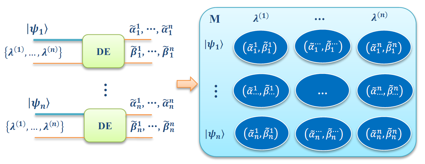
Figure 5: The PPS quadrature demodulation scheme for multiple input fields is shown, where the DE block is shown in Fig. 4.

Now we consider how to construct the states based on $M$ matrix, respectively. Thus we propose a sequence permutation mechanism to simulate each $\left|\Psi\right\rangle$ based on $M$ matrix, which is one of the simplest mechanisms for sequence ergodic ensemble. Assumed $\left|\Psi\right\rangle$ contains $n$ classical optical fields with $n$ PPSs, namely the corresponding matrix contains $n$ rows and $n$ columns, the sequence permutation is arranged as

$$R_{1}=\left\{\lambda^{\left(1\right)},\lambda^{\left(2\right)},\ldots,\lambda^{\left(n\right)}\right\},R_{2}=\left\{\lambda^{\left(2\right)},\lambda^{\left(3\right)},\ldots,\lambda^{\left(1\right)}\right\},\ldots,R_{n}=\left\{\lambda^{\left(n\right)},\lambda^{\left(1\right)},\ldots,\lambda^{\left(n-1\right)}\right\}.$$ (30)

As shown in Fig. 6, we can obtain the mode status with same color for same sequence permutation, such as the red color corresponding to $R_{1}$, the blue color corresponding to $R_{2}$, etc. We obtain a direct product of $n$ items for each $R_{r}$, and the simulated quantum state is the superposition of the $n$ product items. Therefore we obtain

$$\left|\Psi\right\rangle = \left(\tilde{\alpha}_{1}^{1}\left|0\right\rangle+\tilde{\beta}_{1}^{1}\left|1\right\rangle\right)\otimes\ldots\otimes\left(\tilde{\alpha}_{n}^{n}\left|0\right\rangle+\tilde{\beta}_{n}^{n}\left|1\right\rangle\right)+\left(\tilde{\alpha}_{1}^{2}\left|0\right\rangle+\tilde{\beta}_{1}^{2}\left|1\right\rangle\right)\otimes\ldots\otimes\left(\tilde{\alpha}_{n}^{1}\left|0\right\rangle+\tilde{\beta}_{n}^{1}\left|1\right\rangle\right)$$ (31)

$$+\ldots+\left(\tilde{\alpha}_{1}^{n}\left|0\right\rangle+\tilde{\beta}_{1}^{n}\left|1\right\rangle\right)\otimes\ldots\otimes\left(\tilde{\alpha}_{n}^{n-1}\left|0\right\rangle+\tilde{\beta}_{n}^{n-1}\left|1\right\rangle\right),$$

where $\left(\tilde{\alpha}_{i}^{j},\tilde{\beta}_{i}^{j}\right)$ is the mode status obtained from the matrix $M\left(\tilde{\alpha}_{i}^{j},\tilde{\beta}_{i}^{j}\right)$.

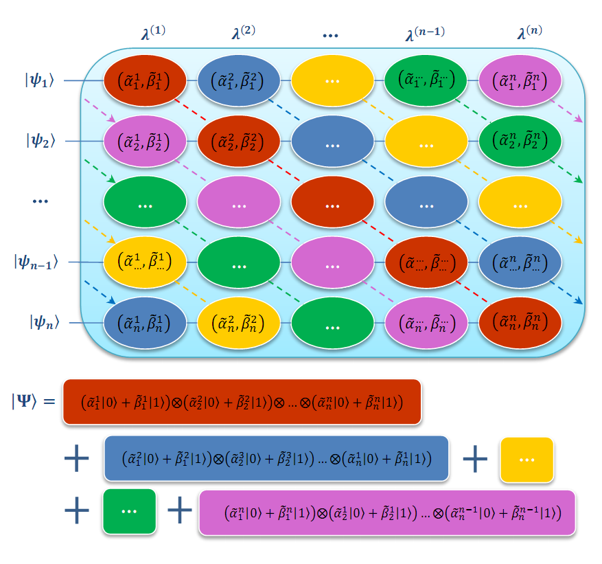
Figure 6: The scheme to simulate quantum state is shown, the mode status matrix $M\left(\tilde{\alpha}_{i}^{j},\tilde{\beta}_{i}^{j}\right)$ related to $i$th classical optical field and the reference PPS $\lambda^{\left(j\right)}$, in which the mode status with same color for same sequence permutation.

It is noteworthy that the mechanism we proposed above is one of the feasible ways to simulate the quantum state based on the mode status matrix. Other mechanisms may also work, as long as a sequence ergodic ensemble is obtained in the mechanism. The sequence permutation mechanism above can successfully simulate many quantum states, including the product states, Bell states, GHZ states and W states. We will discuss the related contents in next subsection.

II.3 Simulations of several typical quantum states

In this subsection, we discuss classical simulations of several typical quantum states, including product state, Bell states, GHZ state and W state.

II.3.1 Product state

First, we discuss classical simulation of $n$ quantum product state. The simulation fields are shown as follows

$$\left|\psi_{1}\right\rangle = e^{i\lambda^{\left(1\right)}}\left(\left|0\right\rangle+\left|1\right\rangle\right),$$

$$......$$

$$\left|\psi_{n}\right\rangle = e^{i\lambda^{\left(n\right)}}\left(\left|0\right\rangle+\left|1\right\rangle\right).$$

By employing the scheme as shown in Fig. 6, we obtain the mode status matrix

$$M\left(\tilde{\alpha}_{i}^{j},\tilde{\beta}_{i}^{j}\right)=\left(\begin{array}[]{ccc}\left(1,1\right)&&0\\ &\ddots&\\ 0&&\left(1,1\right)\end{array}\right),$$ (33)

which demonstrates that each classical optical field is the superposition of two orthogonal modes and no entanglement is involved. According to Eq. (31), we obtain

$$\left|\Psi\right\rangle = \left(\left|0\right\rangle+\left|1\right\rangle\right)\otimes\ldots\otimes\left(\left|0\right\rangle+\left|1\right\rangle\right)$$

$$= \left|0\ldots 0\right\rangle+\left|0\ldots 1\right\rangle+\ldots+\left|1\ldots 1\right\rangle,$$

where $\left|i_{1}\ldots i_{n}\right\rangle\equiv\left|i_{1}\right\rangle\otimes\ldots\otimes\left|i_{n}\right\rangle,\left(i_{n}=0\ or\ 1\right)$, which is same as a quantum product state expect a normalization factor.

II.3.2 Bell states

Now we discuss classical simulation of one of the four Bell states $\left|\Psi^{+}\right\rangle=\frac{1}{\sqrt{2}}\left(\left|0_{1}\right\rangle\left|0_{2}\right\rangle+\left|1_{1}\right\rangle\left|1_{2}\right\rangle\right)$, which contains two classical optical fields as follows

$$\left|\psi_{1}\right\rangle = e^{i\lambda^{\left(1\right)}}\left|0\right\rangle+e^{i\lambda^{\left(2\right)}}\left|1\right\rangle,$$ (35)

$$\left|\psi_{2}\right\rangle = e^{i\lambda^{\left(2\right)}}\left|0\right\rangle+e^{i\lambda^{\left(1\right)}}\left|1\right\rangle.$$

By employing the scheme as shown in Fig. 6, we obtain the mode status matrix

$$M\left(\tilde{\alpha}_{i}^{j},\tilde{\beta}_{i}^{j}\right)=\left(\begin{array}[]{cc}\left(1,0\right)&\left(0,1\right)\\ \left(0,1\right)&\left(1,0\right)\end{array}\right).$$ (36)

We note that in this case, the mode status matrix is irreducible, which corresponds to an entanglement state. According to the sequence permutation mechanism, we obtain that $R_{1}=\{\lambda^{\left(1\right)},\lambda^{\left(2\right)}\}$ and $R_{2}=\{\lambda^{\left(2\right)},\lambda^{\left(1\right)}\}$. Based on the mode status matrix, for the selection of $R_{1}$, we obtain $\left|0\right\rangle\otimes\left|0\right\rangle$; for the selection of $R_{2}$, we obtain $\left|1\right\rangle\otimes\left|1\right\rangle$. If we randomly choose one selection between $R_{1}$ and $R_{2}$, we can randomly obtain one result between $\left|0\right\rangle\otimes\left|0\right\rangle$ and $\left|1\right\rangle\otimes\left|1\right\rangle$, which is similar with the case of quantum measurement for the Bell state $\left|\Psi^{+}\right\rangle$. We can simulate the state except a norm based on the mode status matrix

$$\left|\Psi^{+}\right\rangle = \left(\tilde{\alpha}_{1}^{1}\left|0\right\rangle+\tilde{\beta}_{1}^{1}\left|1\right\rangle\right)\otimes\left(\tilde{\alpha}_{2}^{2}\left|0\right\rangle+\tilde{\beta}_{2}^{2}\left|1\right\rangle\right)+\left(\tilde{\alpha}_{1}^{2}\left|0\right\rangle+\tilde{\beta}_{1}^{2}\left|1\right\rangle\right)\otimes\left(\tilde{\alpha}_{2}^{1}\left|0\right\rangle+\tilde{\beta}_{2}^{1}\left|1\right\rangle\right)$$ (37)

$$= \left|00\right\rangle+\left|11\right\rangle$$

which is same as the Bell state $\left|\Psi^{+}\right\rangle$ expect a normalization factor.

In quantum mechanics, another Bell state $\left|\Phi^{+}\right\rangle$ can be obtained from $\left|\Psi^{+}\right\rangle$ by performing the unitary transformation $\sigma_{x}:\left|0\right\rangle\leftrightarrow\left|1\right\rangle$ on one of the particles. Using the same method, we perform an unitary transformation on $\left|\psi_{b}\right\rangle$ to flip its modes $\left|0\right\rangle\leftrightarrow\left|1\right\rangle$. Thus we obtain two classical optical fields as follows

$$\left|\psi_{1}\right\rangle = e^{i\lambda^{\left(1\right)}}\left|0\right\rangle+e^{i\lambda^{\left(2\right)}}\left|1\right\rangle,$$ (38)

$$\left|\psi_{2}\right\rangle = e^{i\lambda^{\left(2\right)}}\left|1\right\rangle+e^{i\lambda^{\left(1\right)}}\left|0\right\rangle.$$

By employing the scheme as shown in Fig. 6, we obtain the mode status matrix

$$M\left(\tilde{\alpha}_{i}^{j},\tilde{\beta}_{i}^{j}\right)=\left(\begin{array}[]{cc}\left(1,0\right)&\left(0,1\right)\\ \left(1,0\right)&\left(0,1\right)\end{array}\right).$$ (39)

According to the sequence permutation mechanism, here we obtain $R_{1}$ and $R_{2}$ again. As the mode status matrix is different, for $R_{1}$, the result turns to be $\left|0\right\rangle\otimes\left|1\right\rangle$; for $R_{2}$, we obtain $\left|1\right\rangle\otimes\left|0\right\rangle$. If we randomly choose one selection between $R_{1}$ and $R_{2}$, we can also randomly obtain one result between $\left|0\right\rangle\otimes\left|1\right\rangle$ and $\left|0\right\rangle\otimes\left|1\right\rangle$, which is similar with the case of quantum measurement for the Bell state $\left|\Phi^{+}\right\rangle$. We can simulate the state

$$\left|\Phi^{+}\right\rangle = \left(\tilde{\alpha}_{1}^{1}\left|0\right\rangle+\tilde{\beta}_{1}^{1}\left|1\right\rangle\right)\otimes\left(\tilde{\alpha}_{2}^{2}\left|0\right\rangle+\tilde{\beta}_{2}^{2}\left|1\right\rangle\right)+\left(\tilde{\alpha}_{1}^{2}\left|0\right\rangle+\tilde{\beta}_{1}^{2}\left|1\right\rangle\right)\otimes\left(\tilde{\alpha}_{2}^{1}\left|0\right\rangle+\tilde{\beta}_{2}^{1}\left|1\right\rangle\right)$$ (40)

$$= \left|10\right\rangle+\left|01\right\rangle$$

which is same as the Bell state $\left|\Phi^{+}\right\rangle$ expect a normalization factor. For other two Bell states $\left|\Psi^{-}\right\rangle$ and $\left|\Phi^{-}\right\rangle$, they can be obtained from $\left|\Psi^{+}\right\rangle$ and $\left|\Phi^{+}\right\rangle$ by using a $\pi$ phase transformation. We can distinguish $\left|\Psi^{-}\right\rangle$ and $\left|\Phi^{-}\right\rangle$ from $\left|\Psi^{+}\right\rangle$ and $\left|\Phi^{+}\right\rangle$ by using the signal polarity of quadrature demodulation.

II.3.3 GHZ state

For tripartite systems there are only two different classes of genuine tripartite entanglement, the GHZ class and the W class Greenberger ; Nielsen . First we discuss the classical simulation of GHZ state $\left|\Psi_{GHZ}\right\rangle=\frac{1}{\sqrt{2}}\left(\left|0_{1}\right\rangle\left|0_{2}\right\rangle\left|0_{3}\right\rangle+\left|1_{1}\right\rangle\left|1_{2}\right\rangle\left|1_{3}\right\rangle\right)$, which contains three classical optical fields as follows

$$\left|\psi_{1}\right\rangle = e^{i\lambda^{\left(1\right)}}\left|0\right\rangle+e^{i\lambda^{\left(2\right)}}\left|1\right\rangle,$$ (41)

$$\left|\psi_{2}\right\rangle = e^{i\lambda^{\left(2\right)}}\left|0\right\rangle+e^{i\lambda^{\left(3\right)}}\left|1\right\rangle,$$

$$\left|\psi_{3}\right\rangle = e^{i\lambda^{\left(3\right)}}\left|0\right\rangle+e^{i\lambda^{\left(1\right)}}\left|1\right\rangle.$$

Performing the scheme as shown in Fig. 6, we obtain the mode status matrix

$$M\left(\tilde{\alpha}_{i}^{j},\tilde{\beta}_{i}^{j}\right)=\left(\begin{array}[]{ccc}\left(1,0\right)&\left(0,1\right)&0\\ 0&\left(1,0\right)&\left(0,1\right)\\ \left(0,1\right)&0&\left(1,0\right)\end{array}\right).$$ (42)

According to the sequence permutation mechanism, we obtain that $R_{1}=\{\lambda^{\left(1\right)},\lambda^{\left(2\right)},\lambda^{\left(3\right)}\}$, $R_{2}=\{\lambda^{\left(2\right)},\lambda^{\left(3\right)},\lambda^{\left(1\right)}\}$ and $R_{3}=\{\lambda^{\left(3\right)},\lambda^{\left(1\right)},\lambda^{\left(2\right)}\}$. Based on the mode status matrix, for the selection of $R_{1}$, we obtain $\left|0\right\rangle\otimes\left|0\right\rangle\otimes\left|0\right\rangle$; for the selection of $R_{2}$, we obtain $\left|1\right\rangle\otimes\left|1\right\rangle\otimes\left|1\right\rangle$; for the selection of $R_{3}$, we obtain nothing. Thus we can simulate the state based on the mode status matrix

$$\left|\Psi_{GHZ}\right\rangle = \left(\tilde{\alpha}_{1}^{1}\left|0\right\rangle+\tilde{\beta}_{1}^{1}\left|1\right\rangle\right)\otimes\left(\tilde{\alpha}_{2}^{2}\left|0\right\rangle+\tilde{\beta}_{2}^{2}\left|1\right\rangle\right)\otimes\left(\tilde{\alpha}_{3}^{3}\left|0\right\rangle+\tilde{\beta}_{3}^{3}\left|1\right\rangle\right)$$

$$+\left(\tilde{\alpha}_{1}^{2}\left|0\right\rangle+\tilde{\beta}_{1}^{2}\left|1\right\rangle\right)\otimes\left(\tilde{\alpha}_{2}^{3}\left|0\right\rangle+\tilde{\beta}_{2}^{3}\left|1\right\rangle\right)\otimes\left(\tilde{\alpha}_{3}^{1}\left|0\right\rangle+\tilde{\beta}_{3}^{1}\left|1\right\rangle\right)$$

$$= \left|000\right\rangle+\left|111\right\rangle.$$

II.3.4 W state

Then we discuss the classical simulation of W state,

$$\left|\Psi_{W}\right\rangle=\frac{1}{\sqrt{3}}\left(\left|1_{1}\right\rangle\left|0_{2}\right\rangle\left|0_{3}\right\rangle+\left|0_{1}\right\rangle\left|1_{2}\right\rangle\left|0_{3}\right\rangle+\left|0_{1}\right\rangle\left|0_{2}\right\rangle\left|1_{3}\right\rangle\right),$$ (44)

which contains three classical optical fields as follows

$$\left|\psi_{1}\right\rangle = e^{i\lambda^{\left(1\right)}}\left|1\right\rangle+e^{i\lambda^{\left(2\right)}}\left|0\right\rangle+e^{i\lambda^{\left(3\right)}}\left|0\right\rangle,$$ (45)

$$\left|\psi_{2}\right\rangle = e^{i\lambda^{\left(1\right)}}\left|1\right\rangle+e^{i\lambda^{\left(2\right)}}\left|0\right\rangle+e^{i\lambda^{\left(3\right)}}\left|0\right\rangle,$$

$$\left|\psi_{3}\right\rangle = e^{i\lambda^{\left(1\right)}}\left|1\right\rangle+e^{i\lambda^{\left(2\right)}}\left|0\right\rangle+e^{i\lambda^{\left(3\right)}}\left|0\right\rangle.$$

It is noteworthy that the three classical optical fields can be produced from one single field by using two beam splitters, which is quite similar with the generation of W state in quantum mechanics. Performing the same scheme, we obtain the mode status matrix

$$M\left(\tilde{\alpha}_{i}^{j},\tilde{\beta}_{i}^{j}\right)=\left(\begin{array}[]{ccc}\left(0,1\right)&\left(1,0\right)&\left(1,0\right)\\ \left(0,1\right)&\left(1,0\right)&\left(1,0\right)\\ \left(0,1\right)&\left(1,0\right)&\left(1,0\right)\end{array}\right).$$ (46)

According to the sequence permutation mechanism, we use $R_{1}$, $R_{2}$ and $R_{3}$ again. Based on the mode status matrix, we obtain $\left|1\right\rangle\otimes\left|0\right\rangle\otimes\left|0\right\rangle$, $\left|0\right\rangle\otimes\left|0\right\rangle\otimes\left|1\right\rangle$, $\left|0\right\rangle\otimes\left|1\right\rangle\otimes\left|0\right\rangle$ for the selection of $R_{1}$, $R_{2}$, $R_{3}$, respectively. We find an interesting fact that when we obtain the state $\left|1\right\rangle$ of the first field, $R_{1}$ must be selected, thus only the $\left|0\right\rangle\otimes\left|0\right\rangle$ state can be obtained from the other two fields; otherwise when we obtain the state $\left|0\right\rangle$ of the first field, the selection can be $R_{2}$ or $R_{3}$, thus the state of $\left|0\right\rangle\otimes\left|1\right\rangle+\left|1\right\rangle\otimes\left|0\right\rangle$ can be obtained from the other two fields. This fact is quite similar with the case of quantum measurement and the collapse phenomenon for W state in quantum mechanics. We can simulate the state based on the mode status matrix expect a normalization factor,

$$\left|\Psi_{W}\right\rangle = \left(\tilde{\alpha}_{1}^{1}\left|0\right\rangle+\tilde{\beta}_{1}^{1}\left|1\right\rangle\right)\otimes\left(\tilde{\alpha}_{2}^{2}\left|0\right\rangle+\tilde{\beta}_{2}^{2}\left|1\right\rangle\right)\otimes\left(\tilde{\alpha}_{3}^{3}\left|0\right\rangle+\tilde{\beta}_{3}^{3}\left|1\right\rangle\right)$$

$$+\left(\tilde{\alpha}_{1}^{2}\left|0\right\rangle+\tilde{\beta}_{1}^{2}\left|1\right\rangle\right)\otimes\left(\tilde{\alpha}_{2}^{3}\left|0\right\rangle+\tilde{\beta}_{2}^{3}\left|1\right\rangle\right)\otimes\left(\tilde{\alpha}_{3}^{1}\left|0\right\rangle+\tilde{\beta}_{3}^{1}\left|1\right\rangle\right)$$

$$+\left(\tilde{\alpha}_{1}^{3}\left|0\right\rangle+\tilde{\beta}_{1}^{3}\left|1\right\rangle\right)\otimes\left(\tilde{\alpha}_{2}^{1}\left|0\right\rangle+\tilde{\beta}_{2}^{1}\left|1\right\rangle\right)\otimes\left(\tilde{\alpha}_{3}^{2}\left|0\right\rangle+\tilde{\beta}_{3}^{2}\left|1\right\rangle\right)$$

$$= \left|100\right\rangle+\left|010\right\rangle+\left|001\right\rangle.$$

Above we discussed the possibility of simulating several typical quantum states by classical fields and mechanism of coherent detection.

III Simulation of quantum computation

In this chapter we will propose a method to simulate quantum computation. In quantum computation, any quantum state can be obtained from initial states by using unitary transformation of universal gates. Similarly, we can construct simulation of all kinds of quantum states by using a gate array, such as GHZ state and W state, even to realize Shor’s algorithm and Grover’s algorithm.

III.1 Gate array model to simulate quantum computation

In Ref. Fu1 , a constructure pathway of simulation states is shown. Here we use the same model as shown Fig. 7, however a gate array (GA) is proposed instead of the unitary transformation to produce simulation states. Now we discuss some basic units of gate array model.

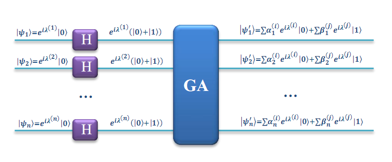
Figure 7: A gate array model to simulate quantum computation is shown, where GA denotes the gate array.

(1) Combiner and splitter

Different from quantum state, we can conveniently combine and split a classical field by using an optical splitter device. Therefore we define two basic device as combiner and splitter as shown in Fig. 8 (a) and (b), respectively.

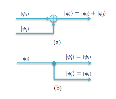
Figure 8: Two basic devices (a) combiner and (b) splitter are shown.

(b) Mode control Gates

Further, we define $4$ kinds of mode control gates as selective mode transit devices with one input and one output as shown in Fig. 9. They are defined by following:

$$\mathbf{Gate}A : \left|\psi_{i}\right\rangle=e^{i\lambda^{\left(i\right)}}\left(\left|0\right\rangle+\left|1\right\rangle\right)\rightarrow\left|\psi_{i}^{\prime}\right\rangle=0,$$ (48)

$$\mathbf{Gate}B : \left|\psi_{i}\right\rangle=e^{i\lambda^{\left(i\right)}}\left(\left|0\right\rangle+\left|1\right\rangle\right)\rightarrow\left|\psi_{i}^{\prime}\right\rangle=e^{i\lambda^{\left(i\right)}}\left|0\right\rangle,$$

$$\mathbf{Gate}C : \left|\psi_{i}\right\rangle=e^{i\lambda^{\left(i\right)}}\left(\left|0\right\rangle+\left|1\right\rangle\right)\rightarrow\left|\psi_{i}^{\prime}\right\rangle=e^{i\lambda^{\left(i\right)}}\left|1\right\rangle,$$

$$\mathbf{Gate}D : \left|\psi_{i}\right\rangle=e^{i\lambda^{\left(i\right)}}\left(\left|0\right\rangle+\left|1\right\rangle\right)\rightarrow\left|\psi_{i}^{\prime}\right\rangle=e^{i\lambda^{\left(i\right)}}\left(\left|0\right\rangle+\left|1\right\rangle\right).$$

Figure 9: Mode control gates as selective mode transit devices are shown.

Now we will discuss a basic structure of gate array model. According to Sec. II.3.2, we can simulation of quantum states by using sequence permutations. Similar to field programmable gate array (FPGA), we propose a simple structure of gate array to obtain permutation structure as shown in Fig. 10. Gates $G_{kj}$ constituted by the basic units can transform $\left|\psi_{k}\right\rangle$ to achieve certain $\left|\psi_{k}^{\prime}\right\rangle$. It is easy to know that a sequence permutation with circulation of $p+1$ needs at least $p$ combiner devices and $2p$ control gates. Any states is capable to be constructed by applying this structure that will be strictly proved in future paper.

Figure 10: A basic structrue of gate array model is shown.

Finally, we illustrate two gate array models to transform product states to GHZ state and W state as shown in Fig. 11.

Figure 11: Gate array models to transform product states to (a) GHZ state and (b) W state are shown.

III.2 Simulation of quantum algorithm

III.2.1 Shor’s Algorithm

Shor’s algorithm is a quantum algorithm for integer factorization that runs only in polynomial time on a quantum computer Shor ; Shor2 . Specifically it takes time and quantum gates of order $O((\log N)^{2}(\log\log N)(\log\log\log N))$ using fast multiplication, demonstrating that the integer factorization problem can be efficiently solved on a quantum computer and is thus in the complexity class BQP.

In this chapter, we discuss the simulation of Shor’s algorithm. A algorithm similar Shor’s algorithm is demonstrated, that factored $N=15$ into $3\times 5$, using the gate array model with $8$ classical optical fields. First, we chose a random number $a$ coprime with $15$, for example $a=7$. We define a function as followed

$$f\left(x\right)=a^{x}modN=7^{x}mod15.$$ (49)

The key step of the Shor’s algorithm is to obtain the period $r$ to satisfy

$$f\left(x+r\right)=7^{x+r}mod15=7^{x}mod15=f\left(x\right).$$ (50)

In order to construct $f\left(x\right)$, we prepare $8$ classical optical fields modulated with $8$ PPSs:

$$\left|\psi_{k}\right\rangle=e^{i\lambda^{\left(k\right)}}\left(\left|0\right\rangle+\left|1\right\rangle\right),k=1\ldots 8.$$ (51)

We can express the product state as followed:

$$\left|\Psi\right\rangle=\left|\psi_{1}\right\rangle\otimes\ldots\otimes\left|\psi_{8}\right\rangle=\sum\limits_{j=0}^{255}\left|j\right\rangle.$$ (52)

Further, we construct a gate array model as shown in Fig. 12. After passing through the gate array and the classical fields will become the forms as follows:

$$\left|\psi_{1}^{\prime}\right\rangle = \left(e^{i\lambda^{\left(1\right)}}+e^{i\lambda^{\left(2\right)}}+e^{i\lambda^{\left(3\right)}}+e^{i\lambda^{\left(4\right)}}\right)\left(\left|0\right\rangle+\left|1\right\rangle\right),$$ (53)

$$\left|\psi_{2}^{\prime}\right\rangle = \left(e^{i\lambda^{\left(2\right)}}+e^{i\lambda^{\left(3\right)}}+e^{i\lambda^{\left(4\right)}}+e^{i\lambda^{\left(5\right)}}\right)\left(\left|0\right\rangle+\left|1\right\rangle\right),$$

$$\left|\psi_{3}^{\prime}\right\rangle = \left(e^{i\lambda^{\left(3\right)}}+e^{i\lambda^{\left(4\right)}}\right)\left|0\right\rangle+\left(e^{i\lambda^{\left(5\right)}}+e^{i\lambda^{\left(6\right)}}\right)\left|1\right\rangle,$$

$$\left|\psi_{4}^{\prime}\right\rangle = \left(e^{i\lambda^{\left(4\right)}}+e^{i\lambda^{\left(6\right)}}\right)\left|0\right\rangle+\left(e^{i\lambda^{\left(5\right)}}+e^{i\lambda^{\left(7\right)}}\right)\left|1\right\rangle,$$

$$\left|\psi_{5}^{\prime}\right\rangle = \left(e^{i\lambda^{\left(5\right)}}+e^{i\lambda^{\left(6\right)}}+e^{i\lambda^{\left(7\right)}}\right)\left|0\right\rangle+e^{i\lambda^{\left(8\right)}}\left|1\right\rangle,$$

$$\left|\psi_{6}^{\prime}\right\rangle = e^{i\lambda^{\left(6\right)}}\left|0\right\rangle+\left(e^{i\lambda^{\left(7\right)}}+e^{i\lambda^{\left(8\right)}}+e^{i\lambda^{\left(1\right)}}\right)\left|1\right\rangle,$$

$$\left|\psi_{7}^{\prime}\right\rangle = \left(e^{i\lambda^{\left(7\right)}}+e^{i\lambda^{\left(1\right)}}+e^{i\lambda^{\left(2\right)}}\right)\left|0\right\rangle+e^{i\lambda^{\left(8\right)}}\left|1\right\rangle,$$

$$\left|\psi_{8}^{\prime}\right\rangle = \left(e^{i\lambda^{\left(8\right)}}+e^{i\lambda^{\left(2\right)}}\right)\left|0\right\rangle+\left(e^{i\lambda^{\left(1\right)}}+e^{i\lambda^{\left(3\right)}}\right)\left|1\right\rangle.$$

By using the quadrature demodulation, we can obtain the mode status matrix:

$$M\left(\tilde{\alpha}_{i}^{j},\tilde{\beta}_{i}^{j}\right)=\left(\begin{array}[]{cccccccc}\left(1,1\right)&\left(1,1\right)&\left(1,1\right)&\left(1,1\right)&0&0&0&0\\ 0&\left(1,1\right)&\left(1,1\right)&\left(1,1\right)&\left(1,1\right)&0&0&0\\ 0&0&\left(1,0\right)&\left(1,0\right)&\left(0,1\right)&\left(0,1\right)&0&0\\ 0&0&0&\left(1,0\right)&\left(0,1\right)&\left(1,0\right)&\left(0,1\right)&0\\ 0&0&0&0&\left(1,0\right)&\left(1,0\right)&\left(1,0\right)&\left(0,1\right)\\ \left(0,1\right)&0&0&0&0&\left(1,0\right)&\left(0,1\right)&\left(0,1\right)\\ \left(1,0\right)&\left(1,0\right)&0&0&0&0&\left(1,0\right)&\left(0,1\right)\\ \left(0,1\right)&\left(1,0\right)&\left(0,1\right)&0&0&0&0&\left(1,0\right)\end{array}\right)$$ (54)

Using the scheme mentioned in Sec. II.2, we can obtain the simulated states:

$$\left|\Psi^{\prime}\right\rangle = \left(\left|0\right\rangle+\left|4\right\rangle+\left|8\right\rangle+\left|12\right\rangle\right)\left|1\right\rangle$$

$$+\left(\left|1\right\rangle+\left|5\right\rangle+\left|9\right\rangle+\left|13\right\rangle\right)\left|7\right\rangle$$

$$+\left(\left|2\right\rangle+\left|6\right\rangle+\left|10\right\rangle+\left|14\right\rangle\right)\left|4\right\rangle$$

$$+\left(\left|3\right\rangle+\left|7\right\rangle+\left|11\right\rangle+\left|15\right\rangle\right)\left|13\right\rangle.$$

There are four kinds of superposition classified from last four qubits containing the values of $f\left(x\right)$ ($\left|1\right\rangle,\left|7\right\rangle,\left|4\right\rangle$ and $\left|13\right\rangle$) in output states, which means the period of $f\left(x\right)=7^{x}mod15$ is $r=4$. It is worth noting that, different from quantum computing, we obtain the expected period of without operating quantum Fourier transformation. The remaining task is much easier. Because $N=15,a=7,r=4$, we obtain

$$\gcd\left(a^{\frac{r}{2}}\pm 1,N\right)=\gcd\left(7^{\frac{r}{2}}\pm 1,15\right)=\gcd\left(49\pm 1,15\right),$$ (56)

where $\gcd(48,15)=3$, and $\gcd(50,15)=5$. Finally, we can deduced that $N\left(15\right)=3\times 5$.

Here, this is the simulation of quantum Shor’s algorithm. Apparently, this algorithm obtains the period of $f\left(x\right)$ without quantum fourier transform and takes time and gates of order $O(\left(\log N\right)^{2})$ by rough estimation. We will discuss this problem in detail in future paper.

Figure 12: A gate array model to realize Shor’s algorithm is shown.

III.2.2 Grover’s Algorithm

Grover’s algorithm is a quantum algorithm for searching an unsorted database with $N$ entries in $O(N^{1/2})$ time and using $O(\log N)$ storage space Grover . Grover’s algorithm demostrates that in the quantum model searching can be done faster than classical computation; in fact its time complexity $O(N^{1/2})$ is asymptotically the fastest possible for searching an unsorted database in the linear quantum model. However, it only provides a quadratic speedup rather than exponential speedup over their classical counterparts.

We now discuss classical simulation of Grover’s algorithm. According to Grover’s algorithm, the steps of the simulation are given as follows. Let $\left|S\right\rangle$ denote the uniform superposition over $N$ states,

$$\left|S\right\rangle=\sum\limits_{i=1}^{N}\left|x_{i}\right\rangle$$ (57)

where $\left|x_{i}\right\rangle$ are the states. For example, we obtain $\left|S\right\rangle$ as a superposition state of $13$ random numbers:

$$\left|S\right\rangle = \left|61\right\rangle+\left|63\right\rangle+\left|117\right\rangle+\left|125\right\rangle+\left|140\right\rangle+\left|142\right\rangle+\left|148\right\rangle$$

$$+\left|212\right\rangle+\left|187\right\rangle+\left|59\right\rangle+\left|238\right\rangle+\left|247\right\rangle+\left|76\right\rangle$$

$$= \left|00111101\right\rangle+\left|00111111\right\rangle+\left|01110101\right\rangle+\left|01111101\right\rangle$$

$$+\left|10001100\right\rangle+\left|10001110\right\rangle+\left|10010100\right\rangle+\left|11010100\right\rangle$$

$$+\left|10111011\right\rangle+\left|00111011\right\rangle+\left|11101110\right\rangle+\left|11110111\right\rangle$$

$$+\left|01001100\right\rangle.$$

We choose $8$ classical fields modulated with $8$ PPSs and after passing through a suitable gate array, that become the forms as follows:

$$\left|\psi_{1}^{\prime}\right\rangle = \left(e^{i\lambda^{\left(1\right)}}+e^{i\lambda^{\left(2\right)}}+e^{i\lambda^{\left(5\right)}}+e^{i\lambda^{\left(8\right)}}\right)\left|0\right\rangle+\left(e^{i\lambda^{\left(3\right)}}+e^{i\lambda^{\left(4\right)}}+e^{i\lambda^{\left(5\right)}}+e^{i\lambda^{\left(6\right)}}+e^{i\lambda^{\left(7\right)}}\right)\left|1\right\rangle,$$ (59)

$$\left|\psi_{2}^{\prime}\right\rangle = \left(e^{i\lambda^{\left(2\right)}}+e^{i\lambda^{\left(4\right)}}+e^{i\lambda^{\left(5\right)}}+e^{i\lambda^{\left(6\right)}}\right)\left|0\right\rangle+\left(e^{i\lambda^{\left(1\right)}}+e^{i\lambda^{\left(3\right)}}+e^{i\lambda^{\left(5\right)}}+e^{i\lambda^{\left(7\right)}}+e^{i\lambda^{\left(8\right)}}\right)\left|1\right\rangle,$$

$$\left|\psi_{3}^{\prime}\right\rangle = \left(e^{i\lambda^{\left(2\right)}}+e^{i\lambda^{\left(5\right)}}+e^{i\lambda^{\left(6\right)}}\right)\left|0\right\rangle+\left(e^{i\lambda^{\left(1\right)}}+e^{i\lambda^{\left(3\right)}}+e^{i\lambda^{\left(4\right)}}+e^{i\lambda^{\left(7\right)}}+e^{i\lambda^{\left(8\right)}}\right)\left|1\right\rangle,$$

$$\left|\psi_{4}^{\prime}\right\rangle = \left(e^{i\lambda^{\left(1\right)}}+e^{i\lambda^{\left(3\right)}}+e^{i\lambda^{\left(6\right)}}+e^{i\lambda^{\left(8\right)}}\right)\left|0\right\rangle+\left(e^{i\lambda^{\left(2\right)}}+e^{i\lambda^{\left(4\right)}}+e^{i\lambda^{\left(5\right)}}+e^{i\lambda^{\left(7\right)}}\right)\left|1\right\rangle,$$

$$\left|\psi_{5}^{\prime}\right\rangle = \left(e^{i\lambda^{\left(3\right)}}+e^{i\lambda^{\left(6\right)}}+e^{i\lambda^{\left(8\right)}}\right)\left|0\right\rangle+\left(e^{i\lambda^{\left(1\right)}}+e^{i\lambda^{\left(2\right)}}+e^{i\lambda^{\left(4\right)}}+e^{i\lambda^{\left(5\right)}}+e^{i\lambda^{\left(6\right)}}+e^{i\lambda^{\left(7\right)}}\right)\left|1\right\rangle,$$

$$\left|\psi_{6}^{\prime}\right\rangle = e^{i\lambda^{\left(2\right)}}\left|0\right\rangle+\left(e^{i\lambda^{\left(1\right)}}+e^{i\lambda^{\left(3\right)}}+e^{i\lambda^{\left(4\right)}}+e^{i\lambda^{\left(5\right)}}+e^{i\lambda^{\left(6\right)}}+e^{i\lambda^{\left(7\right)}}+e^{i\lambda^{\left(8\right)}}\right)\left|1\right\rangle,$$

$$\left|\psi_{7}^{\prime}\right\rangle = \left(e^{i\lambda^{\left(1\right)}}+e^{i\lambda^{\left(2\right)}}+e^{i\lambda^{\left(6\right)}}+e^{i\lambda^{\left(7\right)}}+e^{i\lambda^{\left(8\right)}}\right)\left|0\right\rangle+\left(e^{i\lambda^{\left(1\right)}}+e^{i\lambda^{\left(3\right)}}+e^{i\lambda^{\left(4\right)}}+e^{i\lambda^{\left(5\right)}}+e^{i\lambda^{\left(7\right)}}\right)\left|1\right\rangle,$$

$$\left|\psi_{8}^{\prime}\right\rangle = \left(e^{i\lambda^{\left(2\right)}}+e^{i\lambda^{\left(3\right)}}+e^{i\lambda^{\left(5\right)}}+e^{i\lambda^{\left(7\right)}}\right)\left|0\right\rangle+\left(e^{i\lambda^{\left(1\right)}}+e^{i\lambda^{\left(4\right)}}+e^{i\lambda^{\left(6\right)}}+e^{i\lambda^{\left(8\right)}}\right)\left|1\right\rangle.$$

Due to the scheme mentioned in Sec. II.2, any simulated state must correspond to a certain sequence permutation. Therefore, the problem to determine whether $\left|x\right\rangle$ exists in $\left|S\right\rangle$ become that to search the corresponding sequence permutation. For example, we search the number $\left|x\right\rangle=\left|148\right\rangle=\left|10010100\right\rangle$ in $\left|S\right\rangle$. First, the classical fields of state $\left|S\right\rangle$ pass through a gate array as shown in Fig. 13. Then we obtain the mode status matrix by using the quadrature demodulation:

$$M\left(\tilde{\alpha}_{i}^{j},\tilde{\beta}_{i}^{j}\right)=\left(\begin{array}[]{cccccccc}0&0&\left(0,1\right)&\left(0,1\right)&\left(0,1\right)&\left(0,1\right)&\left(0,1\right)&0\\ 0&\left(1,0\right)&0&\left(1,0\right)&\left(1,0\right)&\left(1,0\right)&0&0\\ 0&\left(1,0\right)&0&0&\left(1,0\right)&\left(1,0\right)&0&0\\ 0&\left(0,1\right)&0&\left(0,1\right)&\left(0,1\right)&0&\left(0,1\right)&0\\ 0&0&\left(1,0\right)&0&0&\left(1,0\right)&0&\left(1,0\right)\\ \left(0,1\right)&0&\left(0,1\right)&\left(0,1\right)&\left(0,1\right)&\left(0,1\right)&\left(0,1\right)&\left(0,1\right)\\ \left(1,0\right)&\left(1,0\right)&0&0&0&\left(1,0\right)&\left(1,0\right)&\left(1,0\right)\\ 0&\left(1,0\right)&\left(1,0\right)&0&\left(1,0\right)&0&\left(1,0\right)&0\end{array}\right)$$ (60)

Finally, it is easy to search only corresponding sequence permutation $R_{4}=\left\{\lambda^{\left(4\right)},\lambda^{\left(5\right)},\lambda^{\left(6\right)},\lambda^{\left(7\right)},\lambda^{\left(8\right)},\lambda^{\left(1\right)},\lambda^{\left(2\right)},\lambda^{\left(3\right)}\right\}$. If we choose $\left|x\right\rangle=\left|240\right\rangle=\left|11110000\right\rangle$, we can obtain the mode status matrix

$$M\left(\tilde{\alpha}_{i}^{j},\tilde{\beta}_{i}^{j}\right)=\left(\begin{array}[]{cccccccc}0&0&\left(0,1\right)&\left(0,1\right)&\left(0,1\right)&\left(0,1\right)&\left(0,1\right)&0\\ \left(0,1\right)&0&\left(0,1\right)&0&\left(0,1\right)&0&\left(0,1\right)&\left(0,1\right)\\ \left(0,1\right)&0&\left(0,1\right)&\left(0,1\right)&0&0&\left(0,1\right)&\left(0,1\right)\\ 0&\left(0,1\right)&0&\left(0,1\right)&\left(0,1\right)&0&\left(0,1\right)&0\\ 0&0&\left(1,0\right)&0&0&\left(1,0\right)&0&\left(1,0\right)\\ 0&\left(1,0\right)&0&0&0&0&0&0\\ \left(1,0\right)&\left(1,0\right)&0&0&0&\left(1,0\right)&\left(1,0\right)&\left(1,0\right)\\ 0&\left(1,0\right)&\left(1,0\right)&0&\left(1,0\right)&0&\left(1,0\right)&0\end{array}\right)$$ (61)

In the mode status matrix, we can not search any corresponding sequence permutation. Therefore we can conclude $\left|x\right\rangle=\left|240\right\rangle$ does not exist in $\left|S\right\rangle$.

Here, this is the simulation of quantum Grover’s algorithm. Different from Grover’s algorithm, this algorithm for searching an unsorted database with $N$ entries in $O(\left(\log N\right)^{2})$ time and using $O(\left(\log N\right)^{2})$ storage space by rough estimation. We will discuss this problem in detail also in future paper.

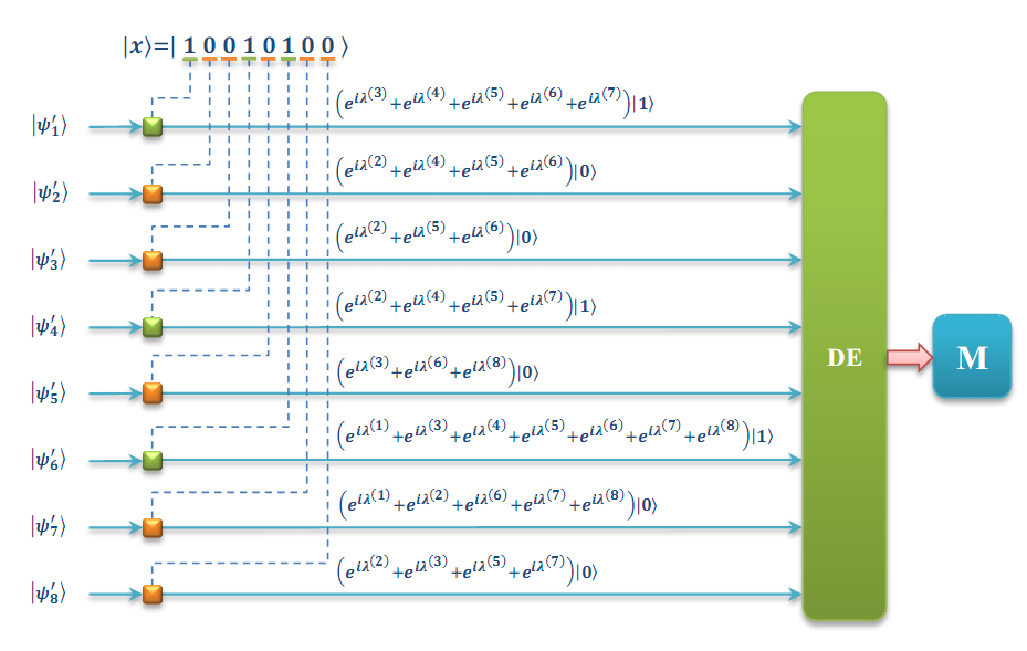
Figure 13: A gate array model to select $\left|x\right\rangle$ from $\left|S\right\rangle$ is shown.

IV Conclusions

In this paper, we have discussed a new scheme to simulate quantum states by using classical optical fields modulated with pseudorandom phase sequences. We first demonstrated that $n$ classical optical fields modulated with $n$ different PPSs can constitute a $n2^{n}$-dimensional Hilbert space that contains tensor product structure similar to quantum systems. Further, by performing quadrature demodulation scheme, we obtained the mode status matrix of the simulating classical optical fields, based on which we proposed a sequence permutation mechanism to simulate the simulated quantum states. Besides, classical simulation of several typical quantum states was discussed, including product state, Bell states, GHZ state and W state. Finally, we generalized our simulation and discussed a generalized gate array model to simulate quantum computation. The research on simulation of quantum states is important, for it not only provides useful insights into fundamental features of quantum mechanics, but also yields new insights into quantum computation and quantum communication.

Fig. 1

The time sequence relationship of the PPS is shown.

Fig. 2

The PPS encoding scheme for one input field is shown, where PNG denotes the pseudorandom number generator and PM denotes the phase modulator.

Fig. 3

The PPS quadrature demodulation scheme for one input field with single mode $e^{i\lambda^{\left(i\right)}}\left|0\right\rangle$ or $e^{i\lambda^{\left(i\right)}}\left|1\right\rangle$ is shown.

Fig. 4

The PPS quadrature demodulation scheme for one field with two orthogonal modes is shown, where the blue block MS denote the mode splitter.

Fig. 5

The PPS quadrature demodulation scheme for multiple input fields is shown, where the DE block is shown in Fig. 4.

Fig. 6

The scheme to simulate quantum state is shown, the mode status matrix $M\left(\tilde{\alpha}_{i}^{j},\tilde{\beta}_{i}^{j}\right)$ related to $i$th classical optical field and the reference PPS $\lambda^{\left(j\right)}$, in which the mode status with same color for same sequence permutation.

Fig. 7

A gate array model to simulate quantum computation is shown, where GA denotes the gate array.

Fig. 8

Two basic devices (a) combiner and (b) splitter are shown.

Fig. 9

Mode control gates as selective mode transit devices are shown.

Fig. 10

A basic structure of gate array model is shown.

Fig. 11

Gate array models to transform product states to (a) GHZ state and (b) W state are shown.

Fig. 12

A gate array model to realize Shor’s algorithm is shown.

Fig. 13

A gate array model to select $\left|x\right\rangle$ from $\left|S\right\rangle$ is shown.

References

- (1) M. R. Garey, D. S. Johnson, Computers and Intractability: A Guide to the Theory of NP-Completeness (A Series of Books in the Mathematical Sciences, W. H. Freeman and Co., San Francisco, 1979)
- (2) M. A. Nielsen and I. L. Chuang, Quantum Computation and Quantum Information (Cambridge University Press, Cambridge, 2000).
- (3) R. Jozsa and N. Linden, Proc. Roy. Soc. London A 459, 2011 (2003); A. Ekert and R. Jozsa, Philos. Trans. R. Soc. London 356, 1769 (1998).
- (4) S. L. Braunstein et al., Phys. Rev. Lett. 83, 1054 (1999); N. Linden and S. Popescu, Phys. Rev. Lett. 87, 047901 (2001); R. Jozsa et al., Proc. R. Soc. A 459, 2011 (2003); G. Vidal, Phys. Rev. Lett. 91, 147902 (2003).
- (5) E. Knill et al., Nature 409, 46 (2001).
- (6) M.A. Nielsen, Phys. Rev. Lett. 93, 040503 (2004).
- (7) D. E. Browne et al., Phys. Rev. Lett. 95, 010501 (2005).
- (8) P. Kok et al., Rev. Mod. Phys. 79, 135 (2007).
- (9) A. Aiello et al., New J. Phys. 17, 043024 (2015); F. Toppel et al., New J. Phys. 16, 073019 (2014); A. Luis, Opt. Commun. 282, 3665 (2009).
- (10) J. Fu and X. Wu, ScienceOpen Research 2015 (DOI: 10.14293/S2199-1006.1.SOR-PHYS.ANVYQZ.v1).
- (11) N. J. Cerf et al., Phys. Rev. A 57, R1478 (1998).
- (12) S. Massar et al., Phys. Rev. A 63, 052305 (2001).
- (13) R. J. C. Spreeuw, Phys. Rev. A 63, 062302 (2001).
- (14) G. Vidal, Phys. Rev. Lett. 91, 147902 (2003).
- (15) A. J. Viterbi, CDMA: principles of spread spectrum communication (Addison-Wesley Wireless Communications Series, Addison-Wesley 1995).
- (16) R. L. Peterson, R. E. Ziemer, and D. E. Borth, Introduction to Spread Spectrum Communications (Prentice-Hall, NJ, 1995).
- (17) G. Proakis, Digital Communications (McGraw Hill, Singapore, 1995).
- (18) P. Shor, in Proc. 35th Annu. Symp. on the Foundations of Computer Science (ed. Goldwasser, S.) 124-134 (IEEE Computer Society Press, Los Alamitos, California, 1994).
- (19) P. Shor, SIAM J. Comput. 26, 1484 (1997).
- (20) L. Grover, In Proc. 28th Annual ACM Symposium on the Theory of Computation 212-219, (ACM Press, New York, 1996); L. Grover, American Journal of Physics 69, 769 (2001).
- (21) J. Fu et al., Phys. Rev. A 70, 042313 (2004); J. Fu, Proceedings of SPIE 5105, 225 (2003).
- (22) D. Dragoman, Prog. Opt. 42, 424 (2002).
- (23) K. F. Lee and J. E. Thomas, Phys. Rev. Lett. 88, 097902 (2002); Phys. Rev. A 69, 052311 (2004).
- (24) D. M. Greenberger et al., Am. J. Phys. 58, 1131 (1990).
- Fig. 1
-