Spontaneous supersymmetry breaking in two dimensional lattice super QCD

Abstract:

We report on a non-perturbative study of two dimensional ${\cal N}=(2,2)$ super QCD. Our lattice formulation retains a single exact supersymmetry at non-zero lattice spacing, and contains $N_{f}$ fermions in the fundamental representation of a $U(N_{c})$ gauge group. The lattice action we employ contains an additional Fayet-Iliopoulos term which is also invariant under the exact lattice supersymmetry. This work constitutes the first numerical study of this theory which serves as a toy model for understanding some of the issues that are expected to arise in four dimensional super QCD. We present evidence that the exact supersymmetry breaks spontaneously when $N_{f}<N_{c}$ in agreement with theoretical expectations.

1 Introduction

In recent years a new approach to the problem of putting supersymmetric theories on the lattice has been developed based on discretization of a topologically twisted version of the continuum theory [1, 2, 3, 4, 5, 6].  Initially the focus was on lattice actions that target pure super Yang-Mills theories in the continuum limit, in particular ${\cal N}=4$ super Yang-Mills [12, 13, 14, 15, 16]. For alternative approaches to numerical studies of ${\cal N}=4$ Yang-Mills see refs. [17, 18, 19, 20]. However in [21] [22] these formulations were extended to the case of theories incorporating fermions transforming in the fundamental representation of the gauge group and hence targeting super QCD. The starting point for these later lattice constructions is a continuum quiver theory containing fields that transform as bifundamentals under a product gauge group $U(N_{c})\times U(N_{f})$. After discretization these bifundamental fields connect two separate lattices and, in the limit that the $U(N_{f})$ gauge coupling is sent to zero, yield a super QCD theory with a global $U(N_{f})$ flavor symmetry. This construction is described in detail in section 3. The lattice action we have employed in this work includes an additional Fayet-Illopoulos term which, while invariant under the exact lattice supersymmetry, generates a potential for the scalar fields. It is straightforward to show that this yields a non-zero vacuum expectation value for the auxiliary field (D term supersymmetry breaking) if $N_{f}<N_{c}$. In section 4. we show the results from numerical simulations of this theory which support this conclusion; we measure a non-zero vacuum energy and show that a light state - the Goldstino- appears in the spectrum of the theory if $N_{f}<N_{c}$. In contrast we show that vacuum energy is zero and this state is absent from the spectrum when $N_{f}>N_{c}$ which is consistent with the prediction that the theory does not spontaneously break supersymmetry in that case.

2 The starting point: twisted ${\cal Q}=8$ SYM in three dimensions

We start from the continuum eight supercharge (${\cal Q}=8$) theory in three dimensions which is written in terms of twisted fields which are completely antisymmetric tensors in spacetime under the twisted SO(3) group. The original two Dirac fermions reappear in the twisted theory as the components of a Kähler-Dirac field $\Psi=\left(\eta,\psi_{a},\chi_{ab},\theta_{abc}\right)$ where the indices $a,b,c=1\ldots 3$. The bosonic sector of the twisted theory comprises a complexified gauge field ${\cal A}_{a}=A_{a}+iB_{a}$ containing the original gauge field $A_{a}$ and an additional vector field $B_{a}$. This additional field contains the three scalars expected of the eight supercharge theory which, being vectors under the R symmetry, transform as a vector field after twisting. The corresponding action $S=S_{\rm exact}+S_{\rm closed}$ where

$$S_{\rm exact} = \frac{1}{g^{2}}\;{\cal Q}\Lambda=\frac{1}{g^{2}}\;{\cal Q}\int d^{3}x{\rm Tr}\left[\chi_{ab}(x){\cal F}_{ab}(x)+\eta(x)\left[{\overline{\cal D}}_{a},{\cal D}_{a}\right]+\frac{1}{2}\eta(x)d(x)\right],$$ (1)

$$S_{\rm closed} = -\;\frac{1}{g^{2}}\int d^{3}x{\rm Tr}\left[\theta_{abc}(x){\overline{\cal D}}_{[c}\chi_{ab]}(x)\right].$$ (2)

Here all fields are in the adjoint representation of a $U(N)$ gauge group $X=\sum_{a=1}^{N^{2}}X_{a}T_{a}$ and we adopt an antihermitian basis for the generators $T_{a}$. ${\cal D}_{a}$ and ${\overline{\cal D}}_{a}$ are the continuum covariant derivatives defined in terms of the complexified gauge fields as ${\cal D}_{a}=\partial_{a}+{\cal A}_{a}$ and ${\overline{\cal D}}_{a}=\partial_{a}+{\overline{\cal A}}_{a}$. The action of the scalar supersymmetry on the fields is given by

$${\cal Q}{\cal A}_{a} = \psi_{a}$$

$${\cal Q}{\overline{\cal A}}_{a} = 0$$

$${\cal Q}\psi_{a} = 0$$

$${\cal Q}\chi_{ab} = -{\overline{\cal F}}_{ab}$$

$${\cal Q}\eta = d$$

$${\cal Q}\theta_{abc} = 0$$ (3)

Notice that we have included an auxiliary field $d(x)$ that allows the algebra to be off-shell nilpotent ${\cal Q}^{2}=0$. This feature then guarantees that $S_{\rm exact}$ is supersymmetric. The equation of motion for this auxiliary field is then

$$d(x)=\left[{\overline{\cal D}}_{a},{\cal D}_{a}\right]$$ (4)

The ${\cal Q}$-invariance of $S_{\rm closed}$ follows from the Bianchi identity

$$\epsilon_{abc}{\overline{\cal D}}_{c}{\overline{\cal F}}_{ab}=0.$$ (5)

To discretize this theory we place all fields on the links of a lattice. This 3d lattice consists of the usual hypercubic vectors plus additional face and body links. In detail these assignments are

continuum field	lattice link
${\cal A}_{a}(x)$	$x\to x+\hat{a}$
${\overline{\cal A}}_{a}(x)$	$x+\hat{a}\to x$
$\psi_{a}(x)$	$x\to x+\hat{a}$
$\chi_{ab}$	$x+\hat{a}+\hat{b}\to x$
$\eta(x)$	$x\to x$
$d(x)$	$x\to x$
$\theta_{abc}$	$x\to x+\hat{a}+\hat{b}+\hat{c}$

The lattice gauge field will be denoted ${\cal U}_{\mu}(x)$ in the following discussion. For the scalar fields $d(x)$, $\eta(x)$ the link degenerates to a single site. Notice that the orientation of a given fermion link field is determined by the even/odd character of its corresponding continuum antisymmetric form. The link character of a field determines its transformation properties under lattice gauge transformations eg. ${\cal U}_{a}(x)\to G(x){\cal U}_{a}(x)G^{\dagger}(x+\hat{a})$. To complete the construction of the lattice action it is necessary to replace continuum covariant derivatives by appropriate gauged lattice difference operators. The necessary prescription was described in [4], [21], [23]. It is essentially determined by the simultaneous requirements that the lattice difference agree with the continuum derivative as the lattice spacing is sent to zero and that it yields expressions that transform as the appropriate link field under lattice gauge transformations. The lattice difference operators acting on a field $f^{(\pm)_{a}}$, where $(\pm)$ corresponding to the orientation of the field, are given by:

$${\cal D}^{(+)}_{a}f^{(+)}_{b_{1},b_{2},...,b_{n}}(x) = {\cal U}_{a}(x)f^{(+)}_{b_{1},b_{2},...,b_{n}}(x+\hat{a})-f^{(+)}_{b_{1},b_{2},...,b_{n}}(x){\cal U}_{a}(x+\hat{b})$$ (6)

$${\cal D}^{(+)}_{a}f^{(-)}_{b_{1},b_{2},...,b_{n}}(x) = {\cal U}_{a}(x+\hat{b})f^{(-)}_{b_{1},b_{2},...,b_{n}}(x+\hat{a})-f^{(-)}_{b_{1},b_{2},...,b_{n}}(x){\cal U}_{a}(x)$$ (7)

$${\overline{\cal D}}^{(+)}_{a}f^{(+)}_{b_{1},b_{2},...,b_{n}}(x) = f^{(+)}_{b_{1},b_{2},...,b_{n}}(x+\hat{a}){\overline{\cal U}}_{a}(x+\hat{b})-{\overline{\cal U}}_{a}(x)f^{(+)}_{b_{1},b_{2},...,b_{n}}(x)$$ (8)

$${\overline{\cal D}}^{(+)}_{a}f^{(-)}_{b_{1},b_{2},...,b_{n}}(x) = f^{(-)}_{b_{1},b_{2},...,b_{n}}(x+\hat{a}){\overline{\cal U}}_{a}(x)-{\cal U}_{a}(x+\hat{b})f^{(-)}_{b_{1},b_{2},...,b_{n}}(x)$$ (9)

$${\cal D}^{(-)}_{a}f^{(\pm)}_{b_{1},b_{2},...,b_{n}}(x) = {\cal D}^{(\pm)}f^{(\pm)}_{b_{1},b_{2},...,b_{n}}(x-\hat{a})$$ (10)

$${\overline{\cal D}}^{(-)}_{a}f^{(\pm)}_{b_{1},b_{2},...,b_{n}}(x) = ={\overline{\cal D}}^{(\pm)}f^{(\pm)}_{b_{1},b_{2},...,b_{n}}(x-\hat{a}),$$ (11)

where $\hat{b}=\sum_{i=1}^{n}\hat{b}_{i}$ in equations (6) to (9). For example the continuum derivative $D_{a}\psi_{b}$ becomes

$${\cal D}^{(+)}_{a}\psi_{b}(x)={\cal U}_{a}(x)\psi_{b}(x+\hat{a})-\psi_{b}(x){\cal U}_{a}(x+\hat{b})$$ (12)

This prescription yields a set of link paths which, when contracted with the link field $\chi_{ab}(x)$, yields a closed loop whose trace is gauge invariant:

$${\rm Tr}\;\left[\chi_{ab}(x)\left({\cal U}_{a}(x)\psi_{b}(x+\hat{a})-\psi_{b}(x){\cal U}_{a}(x+\hat{b})\right)\right]$$ (13)

It has the correct naive continuum limit provided that (in some suitable gauge) we can expand ${\cal U}_{a}(x)=I_{N}+{\cal A}_{a}(x)$. The field strength on the lattice, ${\cal F}_{ab}(x)$, is defined using the forward difference operator as:

$${\cal F}_{ab}(x)={\cal D}^{(+)}_{a}U_{b}(x).$$ (14)

In lattice QCD the unit matrix arising in this expansion is automatic since the link fields take their values in the group. However the constraints of exact lattice supersymmetry require that the lattice gauge fields take their values, like the fermions, in the algebra. In this case the unit matrix can then be interpreted as arising from giving a vev to the trace mode of the original scalar fields $B_{a}$. This feature is required by lattice supersymmetry but is only possible because we are working with a complexified $U(N)$ theory - another indication of the tight connection between twisting and exact supersymmetry. It also implies that the path integral defining the quantum theory will use a flat measure rather than the usual Haar measure employed in conventional lattice gauge theory. Such a prescription would usually break lattice gauge invariance but again complexification comes to the rescue since the Jacobian resulting from a gauge transformation of the $D{\cal U}$ measure cancels against an equivalent one coming from $D{\overline{\cal U}}$.

We now show how to use this three dimensional lattice model to construct a two dimensional quiver theory while maintaining the exact lattice supersymmetry.

3 Two dimensional quivers from three dimensional lattice Yang-Mills

Consider a lattice whose extent in the 3-direction comprises just two 2d slices. Furthermore we shall assume free boundary conditions in the 3-direction so that these two slices are connected by just a single set of links in the 3-direction - those running from $x_{3}=0$ to $x_{3}=1$. Ignoring for the moment any fields that live on these latter links it is clear that the gauge group can be chosen independently on these two slices. We choose a group $U(N_{c})$ for the slice at $x_{3}=0$ and $U(N_{f})$ at $x_{3}=1$ and will henceforth refer to them as the $N_{c}$ and $N_{f}$ lattices. Denoting directions on the 2d slices by Greek indices $\mu,\nu=1,2$ the fields living entirely on these lattices are given by

$$N_{c}\;\;\; : \;\;\;\Psi(x)=\left(\eta,\psi_{\mu},\chi_{\mu\nu}\right),\;\;\;{\cal U}_{\mu}=I_{N_{c}}+{\cal A}_{\mu},\qquad d$$ (15)

$$N_{f}\;\;\; : \;\;\;\hat{\Psi}(\overline{x})=\left(\hat{\eta},\hat{\psi}_{\mu},\hat{\chi}_{\mu\nu}\right),\;\;\;\hat{{\cal U}}_{\mu}=I_{N_{f}}+\hat{{\cal A}},_{\mu},\qquad\hat{d}$$ (16)

In these expressions $x(\overline{x})$ denotes the coordinates on the $N_{c}(N_{f})$ lattice and $1_{N_{c}(N_{f})}$ denote the $N_{c}(N_{f})\times N_{c}(N_{f})$ unit matrix respectively. Now consider fields that live on the links between the $N_{c}$ and $N_{f}$ lattice. These must necessarily transform as bi-fundamentals under $U(N_{c})\times U(N_{f})$. We have,

$$N_{c}\;\times\;N_{f}\;\;\; : \;\;\;\Psi_{\text{bi-fund}}(x,\overline{x})=\left(\psi_{3},\chi_{\mu 3},\theta_{\mu\nu 3}\right)=\left(\lambda,\lambda_{\mu},\lambda_{\mu\nu}\right),\qquad\phi$$ (17)

The second equality in the above equation is a mere change of variables and corresponds to labeling fields according to their two dimensional character. The complete field content of this model is summarized in the table below:

$N_{c}$-lattice	Bi-fundamental fields	$N_{f}$-lattice
$x$	$(x,\overline{x})$ , $(\overline{x},x)$	$\overline{x}$
${\cal A}_{\mu}(x)$	$\phi(x,\overline{x})$	$\hat{{\cal A}_{\mu}}(\overline{x})$
$\eta(x)$	$\lambda(x,\overline{x})$	$\hat{\eta}(\overline{x})$
$\psi_{\mu}(x)$	$\lambda_{\mu}(\overline{x}+\mu,x)$	$\hat{\psi}_{\mu}(\overline{x})$
$\chi_{\mu\nu}(x)$	$\lambda_{\mu\nu}(x,\overline{x}+\mu+\nu)$	$\hat{\chi}_{\mu\nu}(\overline{x})$

Defining G(x) as a group element belonging to $U(N_{c})$ and H(x) to $U(N_{f})$ the lattice gauge transformations for the bi-fundamental fields are as follows:

$$\phi(x) \rightarrow G(x)\phi(x)H^{\dagger}(\overline{x})$$

$$\lambda(x) \rightarrow G(x)\lambda(x)H^{\dagger}(\overline{x})$$

$$\lambda_{\mu}(x) \rightarrow H(\overline{x}+\mu)\lambda_{\mu}(x)G^{\dagger}(x)$$

$$\lambda_{\mu\nu}(x) \rightarrow G(x)\lambda_{\mu\nu}(x)H^{\dagger}(\overline{x}+\mu+\nu)$$ (18)

It is crucial to note that this generalization of the original lattice super Yang-Mills theory to a quiver model is completely consistent with both the quiver gauge symmetries and the exact supersymmetry. For example the 3d term given in eqn. 13 yields a bi-fundamental term of the form

$${\rm Tr}\,\left[\lambda_{\mu}(x)\left({\cal U}_{\mu}(x)\lambda(x+\mu)-\lambda(x)\hat{{\cal U}}_{\mu}(\overline{x})\right)\right]$$ (19)

which is invariant under the the generalized gauge transformations given in eqn. 18. Thus, the above construction lends us a consistent lattice quiver gauge theory containing both adjoint and bi-fundamental fields transforming under a product $U(N_{c})\times U(N_{f})$ gauge group. Consider now setting the $U(N_{f})$ gauge coupling to zero. This sets $\hat{{\cal U}}_{\mu}=I_{N_{f}}$ up to gauge transformations and it is then consistent to set all other fields on the $N_{f}$ lattice to zero. The original $U(N_{f})$ gauge symmetry now becomes a global $U(N_{f})$ flavor symmetry which acts on a set of complex scalar fields $\phi$ transforming in the fundamental representation of the gauge group and their fermionic superpartners $(\lambda,\lambda_{\mu},\lambda_{\mu\nu})$. The situation is depicted in figure 1.

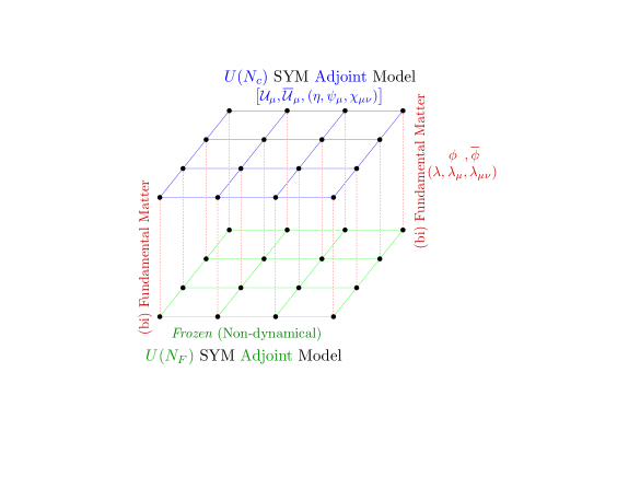
Figure 1: 3d quiver model

At this point we have the freedom to add to the action one further supersymmetric and gauge invariant term - namely $r\sum_{x}{\rm Tr\;}d(x)=r{\cal Q}\sum_{x}{\rm Tr\;}\eta$. This is a Fayet-Iliopoulos term. Its presence changes the equation of motion for the auxiliary field

$$d(x)={\overline{\cal D}}^{(-)}_{\mu}{\cal U}_{\mu}(x)+\phi(x){\overline{\phi}}(x)-rI_{N_{c}}$$ (20)

with $I_{N_{c}}$ a $N_{c}\times N_{c}$ unit matrix. The SUSY transformations for the remaining adjoint and fundamental fields are:

Adjoint Fields	Fundamental fields
${\cal Q}{\cal A}_{\mu}=\psi_{\mu}$	${\cal Q}\phi=\lambda$
${\cal Q}{\overline{\cal A}}_{\mu}=0$	${\cal Q}{\overline{\phi}}=0$
${\cal Q}\psi_{\mu}=0$	${\cal Q}\lambda=0$
${\cal Q}\chi_{\mu\nu}=-{\overline{\cal F}}_{\mu\nu}$	${\cal Q}\lambda_{\mu}=-{\overline{\cal D}}_{\mu}{\overline{\phi}}$
${\cal Q}\eta=d$	${\cal Q}\lambda_{\mu\nu}=0$

After integration over $d$ the Fayet-Iliopoulos term yields a scalar potential term which will play a crucial role in determining whether the system can undergo spontaneous supersymmetry breaking. The final action may be written as

$$S_{\rm adj} = \kappa\sum_{x}{\rm Tr}\left[-{\overline{\cal F}}_{\mu\nu}(x){\cal F}_{\mu\nu}(x)-\frac{1}{2}({\overline{\cal D}}^{(-)}_{\mu}{\cal U}_{\mu})^{2}-\eta(x){\overline{\cal D}}^{(-)}_{\mu}\psi^{\mu}(x)-\chi_{\mu\nu}(x){\cal D}^{(+)}_{[\mu}\psi_{\nu]}(x)\right],$$

$$S_{\rm fund} = \kappa\;\sum_{x}{\rm Tr}\left[-\overline{{\cal D}^{(+)}_{\mu}\phi(x)}{\cal D}^{(+)}_{\mu}\phi(x)-\frac{1}{2}\left[\left(\phi(x){\overline{\phi}}(x)-\rm{rI}\right)^{2}\right]+\left[{\overline{\cal D}}_{\mu}^{(-)}{\cal U}_{\mu}(x)\right]\left(\phi(x){\overline{\phi}}(x)-\rm{rI}\right)\right]$$

$$- \left[\eta(x)\lambda(x){\overline{\phi}}(x)+\left\{\lambda_{\mu}(x){\cal D}^{(+)}_{\mu}\lambda(x)-\lambda_{\mu}(x)\psi_{\mu}(x)\phi(x+\mu)\right\}\right.$$

$$- \left.\left\{\lambda_{\mu\nu}(x)\;{\overline{\cal D}}_{\mu}^{(+)}\lambda_{\nu}(x)-\lambda_{\mu\nu}(x){\overline{\phi}}(x+\mu+\nu)\chi_{\mu\nu}(x)\right\}\right],$$

In practice we have also included the following soft SUSY breaking mass term, $S_{\rm soft}$, in the adjoint action, $S_{\rm adj}$ in equation (LABEL:action-adj):

$$S_{\rm soft}=\mu^{2}\left[\frac{1}{N_{c}}{\rm Tr\;}\left({\overline{\cal U}}_{\mu}{\cal U}_{\mu}\right)-1\right]^{2}.$$ (23)

Such a term is necessary to create a potential for the trace mode of the twisted scalar fields as we have discussed earlier. In principle we should extrapolate $\mu^{2}\to 0$ at the end of the calculation and so we have obtained all our results for a range of $\mu^{2}$. In practice we observe that these soft breaking effects are rather small.

Finally, the lattice coupling $\kappa$ appearing above is given by:

$$\kappa=\frac{N_{c}LT}{2\lambda A}.$$ (24)

Here, $\lambda=g^{2}N_{c}$ is the dimensionful ‘t Hooft coupling, L and T are the numbers of points in each direction of the 2d lattice and $A$ is a continuum area - the importance of interactions in the theory being controlled by the dimensionless combination $\lambda A$. When we later discuss our numerical results we refer to this dimensionless combination as simply $\lambda$.

4 Vacuum Structure and SUSY Breaking Scenarios

Let us return to the equation of motion for the auxiliary field $d(x)$. If we sum the trace of this expression over all lattice sites and take its expectation value we find

$$\langle\sum_{x}{\rm Tr\;}\,d(x)\rangle=\langle\sum_{x}{\rm Tr\;}\,\left(\phi(x){\overline{\phi}}(x)-rI_{N_{c}}\right)\rangle$$ (25)

Since the lefthand side of this expression is the expectation value of the ${\cal Q}$-variation of some operator the question of whether supersymmetry breaks spontaneously or not is determined by whether the righthand side is non-zero. Indeed after we integrate over the auxiliary field $d$ we find a scalar potential of the form

$$S_{\rm Dterm}=\sum_{x,f=1}^{N_{f}}\frac{\kappa}{2}{\rm Tr\;}\left(\phi^{f}(x){\overline{\phi}}^{f}(x)-\rm{rI_{N_{c}}}\right)^{2},$$ (26)

Consider the case where $N_{f}<N_{c}$. Using $SU(N_{c})$ transformations one can diagonalize the $N_{c}\times N_{c}$ matrix $\phi{\overline{\phi}}$. In general it will have $N_{f}$ non-zero real, positive eigenvalues and $N_{c}-N_{f}$ zero eigenvalues. This immediately implies that there is no configuration of the fields $\phi$ where the potential is zero. Indeed the minimum of the potential will have energy $r^{2}(N_{c}-N_{f})$ and corresponds to a situation where $N_{f}$ scalars develop vacuum expectation values breaking the gauge group to $U(N_{c}-N_{f})$. The situation when $N_{f}\geq N_{c}$ is qualitatively different; now the rank of $\phi{\overline{\phi}}$ is at least $N_{c}$ and a zero energy vacuum configuration is possible. In such a situation $N_{c}$ scalars pick up vacuum expectation values and the gauge symmetry is completely broken.

For the case when $N_{f}<N_{c}$ where ${\cal Q}$-supersymmetry is expected to break we would expect the spectrum of the theory to contain a massless fermion - the goldstino [24]. To see how this works in the twisted theory consider the vacuum energy

$$\langle 0|H|0\rangle\neq 0,$$ (27)

which is equivalent to $<\left\{{\cal Q},{\cal O}\right\}>\neq 0$ for some operator ${\cal O}$. In the two dimensional twisted theory the relevant part of the supersymmetry algebra is $\left\{{\cal Q},{\cal Q}_{\mu}\right\}=P_{\mu}$ [25] so that eqn. 27 is equivalent to

$$\langle 0|\left\{{\cal Q},{\cal Q}_{0}\right\}|0\rangle\neq 0,$$ (28)

Note that the equation above involves both the scalar ${\cal Q}$ and the 1-form supercharge ${\cal Q}_{\mu}$. Corresponding to these supercharges are a set of supercurrents, $J$ and $J_{\mu}$ whose form can be derived in the usual manner by varying the continuum twisted action under infinitesimal spacetime dependent susy transformations. This yields gauge invariant supercurrents on the lattice of the following form

$$J(x) = \sum_{\mu}\left[\psi_{\mu}(x){\overline{\cal U}}_{\mu}(x)\right]d(x)+...,$$ (29)

$$J_{0}(x) = \eta(x)d(x)+...,$$ (30)

and using the equations of motion, the auxiliary field d(x) can be replaced by

$$d(x)=\sum_{\mu=1,2}\left[{\overline{\cal D}}_{\mu},{\cal D}_{\mu}\right]+\left[\phi(x){\overline{\phi}}(x)-rI_{N_{c}}\right]$$ (31)

We therefore expect a possible Goldstino signal to manifest itself in the contribution of a light state to the two-point function:

$$C(t)=\langle 0|{\cal O}(x){\cal O}^{\prime}(y)|0\rangle,$$ (32)

where ‘t’ corresponds to $(x^{0}-y^{0})$ and a suitable set of lattice interpolating operators are given by:

$${\cal O}(x)={\rm Tr}\,\left[\sum_{\mu}\psi_{\mu}(x){\overline{\cal U}}_{\mu}(x)\left(\phi(x){\overline{\phi}}(x)-{\rm rI_{N_{c}}}\right)\right].$$ (33)

and

$${\cal O}^{\prime}(y)={\rm Tr}\,\left[\eta(y)\left(\phi(y){\overline{\phi}}(y)-{\rm rI_{N_{c}}}\right)\right].$$ (34)

5 Numerical Results

We employ a RHMC algorithm to simulate our system having first replaced all the twisted fermions in our model by corresponding pseudofermions - see for example [26] [27]. The simulations are performed by imposing anti-periodic (thermal) boundary conditions on the fermions along one of the two space-time directions. This is done to avoid running into the fermion zero modes resulting from the scalar component of the twisted fermion, $\eta$. As discussed in [28] [29] this has the added benefit of ameliorating the sign problem for these lattice theories. This breaks supersymmetry explicitly by a term that vanishes as the lattice volume is increased.

In this section, we contrast results from simulations with $N_{f}=2$, $N_{c}=3$ corresponding to the predicted susy breaking scenario with results from simulations with $N_{f}=3$, $N_{c}=2$ - the susy preserving case. We ran our simulations for three different values of the ‘t Hooft coupling, $\lambda=0.5,1.0$ and 1.5 and observed the same qualitative behavior for the different values of $\lambda$. The results presented in this section correspond to $\lambda=1.0$. The FI parameter, r, is a free parameter and is set to 1.0 for the rest of the discussion.

As a first check, we compared the expectation value of the bosonic action with the theoretical value obtained using a supersymmetric Ward identity

$$<\kappa S_{\rm boson}>=\left(\frac{3}{2}N_{c}^{2}+N_{c}N_{f}\right)V.$$ (35)

In appendix A. we show how to compute this value. Figure 2 shows a plot of the bosonic action for various values of the soft SUSY breaking coupling $\mu$. In principle we should take the limit $\mu\to 0$ although it should be clear from the plot that the $\mu$ dependence is in fact rather weak. We have normalised the data to its value obtained by assuming supersymmetry is unbroken. The red points at the bottom of the figure denote the SUSY preserving case and it can be observed that they agree with the theoretical prediction. This is to be contrasted with the case when $N_{f}<N_{c}$ denoted by the blue points which shows a large deviation from eqn. 35 and is the first sign that supersymmetry is spontaneously broken in this case.

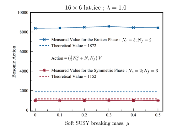
Figure 2: Normalized bosonic action vs soft breaking coupling $\mu$ for $\lambda=1.0$ for a 16x6 lattice

The spatial Polyakov lines shown in figure 3 also show a distinct difference between the $N_{f}<N_{c}$ and $N_{f}>N_{c}$ cases. The red lines where $|P|\approx 1$ correspond to the SUSY preserving case and are consistent with a deconfined or fully Higgsed phase. Indeed the Polyakov line is a topological operator and in a susy preserving phase should be coupling constant independent consistent with what is seen. The blue line in the lower half of the plot corresponds to smaller values which is qualitatively consistent with the predicted partial Higgsing of the gauge field in the phase where supersymmetry is spontaneously broken.

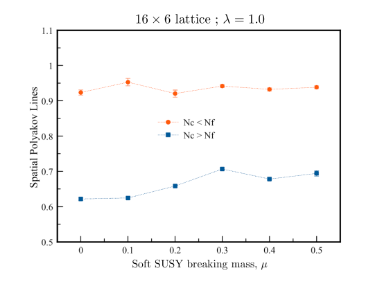
Figure 3: Spatial Polyakov line vs $\mu$ for $\lambda=1.0$ on an 16x6 lattice

One of clearest signals of supersymmetry breaking can be obtained if one considers the equation of motion for the auxiliary field eqn. 26. We expect the susy preserving case to obey

$$\frac{1}{N_{c}}{\rm Tr\;}\left[\phi(x){\overline{\phi}}(x)\right]=1.$$ (36)

The red points, corresponding to ($N_{f}>N_{c}$) are consistent with this over a wide range of $\mu$. We attribute the small residual devaition as $\mu\to 0$ to our use of antiperiodic boundary conditions which inject explicit ${\cal Q}$ susy breaking into the system. The simulations with $N_{f}<N_{c}$ (blue points) however show a clear signal for spontaneous supersymmetry breaking with the value of this quantity deviating dramatically from its supersymmetric value even as $\mu\to 0$.

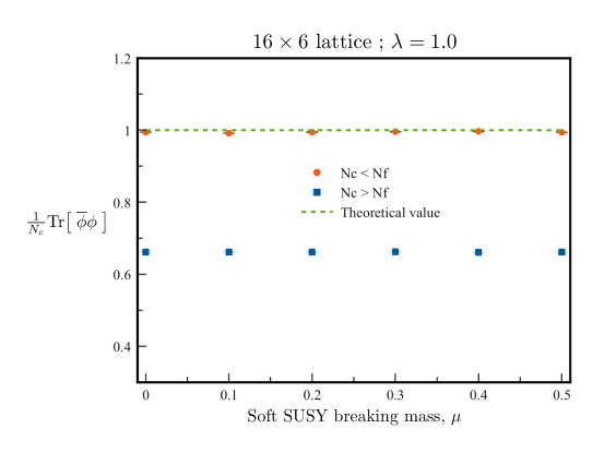
Figure 4: $\frac{1}{N_{c}}{\rm Tr}\phi{\overline{\phi}}$ vs $\mu$ for a ’t Hooft coupling of $\lambda=1.0$ on an 16x6 lattice

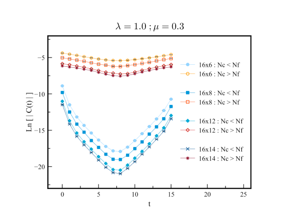
Figure 5: Correlation function C(t) for $\lambda=1.0$ and $\mu=0.3$ on various asymmetric lattices

Finally we turn to our results for a would be Goldstino. We search for this by computing the following two point correlation function

$$C(t)=\sum_{x,y}<O^{\prime}(y,t)O(x,0)>$$ (37)

where $O^{\prime}(y,t)$ and O(x,0) are fermionic operators given by:

$$O(x,0) = \psi_{\mu}(x,0){\cal U}_{\mu}(x,0)\left[\phi(x,0){\overline{\phi}}(x,0)-rI_{N_{c}}\right]$$ (38)

$$O^{\prime}(y,t) = \eta(y,t)\left[\phi(y,t){\overline{\phi}}(y,t)-rI_{N_{c}}\right].$$ (39)

Since it is computationally very cumbersome to evaluate the above correlation function for every lattice site x at the source we instead evaluate the correlator for every lattice site y for a few randomly chosen source points x. In figure 5 we show the logarithm of this correlator as a function of temporal distance for a range of spatial lattice size, $L=6,8,12$ and 14. The anti-periodic boundary condition is applied along the temporal direction corresponding to T=16 and for both $N_{f}>N_{c}$ and $N_{f}<N_{c}$. The approximate linearity of these curves is consistent with the correlator being dominated by a single state in both cases. However when $N_{f}>N_{c}$ the amplitude of this correlator is strongly suppressed relative to the case where $N_{f}<N_{c}$. Furthermore the effective mass extracted from fits to this latter correlator (figure 6) falls as the spatial lattice size (L) increases, consistent with a vanishing mass in the large volume limit. The lines in figure 6 show fits to $1/L$ - the smallest mass consistent with the boundary conditions - the dashed green line is a fit constrained to go through the origin while the dotted red line allows the intercept to float. This is just what we would expect of a would be Goldstino arising from spontaneous breaking of the exact ${\cal Q}$-symmetry.

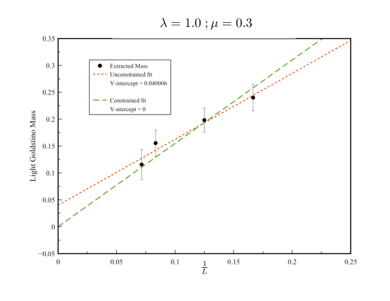
Figure 6: Goldstino mass derived from fits $M_{eff}$ vs inverse transverse lattice size, $L^{-1}$

6 Conclusions

In this paper, we have reported on a numerical study of super QCD in two dimensions. The model in question possesses ${\cal N}=(2,2)$ supersymmetry in the continuum limit while our lattice formulation preserves a single exact supercharge for non zero lattice spacing. It is expected that the single supersymmetry will be sufficient to ensure that full supersymmetry is regained without fine tuning in the continuum limit. This constitutes the first lattice study of a supersymmetric theory containing fields which transform in both the fundamental and adjoint representations of the gauge group. Our lattice action also contains a ${\cal Q}$-exact Fayet-Iliopoulos term which yields a potential for the scalar fields. The lattice theory possesses several exact symmetries; $U(N_{c})$ gauge invariance, ${\cal Q}$-supersymmetry and a global $U(N_{f})$ flavor symmetry.

It is expected that the system will spontaneously break supersymmetry if $N_{f}<N_{c}$. The arguments that lead to this conclusion depend on the inclusion of the Fayet-Iliopoulos term. Such a term is rather natural in our lattice model since the formulation requires $U(N_{c})$ gauge symmetry. Notice, though, that the free energy of the lattice model does not naively depend on the coupling $r$ as long as it is positive since the Fayet-Iliopoulos term is ${\cal Q}$-exact. Our numerical work is fully consistent with this picture; we have examined several supersymmetric Ward identities which clearly distinguish between the $N_{f}<N_{c}$ and $N_{f}>N_{c}$ situations and we have observed a would be Goldstino state in the former case.

There are many directions for future work; inclusion of anti-fundamentals fields is straightforward since it merely corresponds to including the bifundamental fields truncated from the $N_{f}$-lattice. Observations of phase transitions in such models as the parameters are varied can then potentially probe sigma models based on Calabi-Yau hypersurfaces [30]. It is possible that the $SU(N)$ theories could be studied by deforming the moduli space of the lattice theory using ideas similar to those presented in [31]. This would allow direct contact to be made to the continuum calculations of Hori and Tong [32]. Finally the lattice constructions discussed in this paper generalize [33] to three dimensional quiver theories leaving open the possibility of studying 3D super QCD using lattice simulations.

Appendix A Calculating the Bosonic Action

Consider the partition function

$$Z=\int DXe^{-\kappa\left({\cal Q}\Lambda+S_{c}\right)}$$ (40)

where $DX$ denotes the measure over all boson and fermion fields and $S_{c}$ the ${\cal Q}$-closed term. We start by rescaling the field $\theta_{abc}\to\kappa\theta_{abc}$ to remove the coupling $\kappa$ from in front of the ${\cal Q}$-closed term. This yields

$$Z=\kappa^{N_{c}N_{f}V}\int DXe^{-\kappa{\cal Q}\Lambda-S_{c}}=\kappa^{N_{c}N_{f}V}Z^{\prime}$$ (41)

with $V$ the two dimensional volume. Notice that $N_{c}N_{f}$ is the number of fermions at each site resulting from the 3d $\theta$ field. Differentiating with respect to $\kappa$ gives

$$-\frac{\partial\ln{Z}}{\partial\kappa}=-\frac{N_{c}N_{f}V}{\kappa}-\frac{\partial\ln{Z^{\prime}}}{\partial\kappa}$$ (42)

The last term in the righthand side being ${\cal Q}$-exact would yield zero in the original theory containing a $d$-field. However in the action we simulate this field is integrated out yielding instead a contribution of $-\frac{1}{2\kappa}N_{c}^{2}V$ Putting these pieces together we find

$$\kappa<S_{b}>+\kappa<S_{f}>=-N_{c}N_{f}V-\frac{1}{2}N_{c}^{2}V$$ (43)

The expectation value of the fermionic action can be gotten by scaling arguments since the fermions occur only quadratically in the action yielding

$$\kappa<S_{f}>=-\frac{4V}{2}\left(N_{c}^{2}+N_{c}N_{f}\right)$$ (44)

Collecting terms yields the final result quoted previously

$$\kappa<S_{b}>=V\left(\frac{3}{2}N_{c}^{2}+N_{c}N_{f}\right)$$ (45)

- [1] F. Sugino, SuperYang-Mills theories on the two-dimensional lattice with exact supersymmetry, JHEP 0403 (2004) 067, [hep-lat/0401017].
- [2] S. Catterall, A Geometrical approach to N=2 super Yang-Mills theory on the two dimensional lattice, JHEP 0411 (2004) 006, [hep-lat/0410052].
- [3] S. Catterall, Lattice formulation of N=4 super Yang-Mills theory, JHEP 0506 (2005) 027, [hep-lat/0503036].
- [4] S. Catterall, D. B. Kaplan, and M. Unsal, Exact lattice supersymmetry, Phys.Rept. 484 (2009) 71–130, [arXiv:0903.4881].
- [5] A. D’Adda, I. Kanamori, N. Kawamoto, and K. Nagata, Exact extended supersymmetry on a lattice: Twisted N=2 super Yang-Mills in two dimensions, Phys.Lett. B633 (2006) 645–652, [hep-lat/0507029].
- [6] P. H. Damgaard and S. Matsuura, Geometry of Orbifolded Supersymmetric Lattice Gauge Theories, Phys.Lett. B661 (2008) 52–56, [arXiv:0801.2936].
- [7] A. G. Cohen, D. B. Kaplan, E. Katz, and M. Unsal, Supersymmetry on a Euclidean space-time lattice. 1. A Target theory with four supercharges, JHEP 0308 (2003) 024, [hep-lat/0302017].
- [8] A. G. Cohen, D. B. Kaplan, E. Katz, and M. Unsal, Supersymmetry on a Euclidean space-time lattice. 2. Target theories with eight supercharges, JHEP 0312 (2003) 031, [hep-lat/0307012].
- [9] D. B. Kaplan and M. Unsal, A Euclidean lattice construction of supersymmetric Yang-Mills theories with sixteen supercharges, JHEP 0509 (2005) 042, [hep-lat/0503039].
- [10] P. H. Damgaard and S. Matsuura, Classification of supersymmetric lattice gauge theories by orbifolding, JHEP 0707 (2007) 051, [arXiv:0704.2696].
- [11] M. Unsal, Twisted supersymmetric gauge theories and orbifold lattices, JHEP 0610 (2006) 089, [hep-th/0603046].
- [12] S. Catterall, D. Schaich, P. H. Damgaard, T. DeGrand, and J. Giedt, N=4 Supersymmetry on a Space-Time Lattice, Phys.Rev. D90 (2014), no. 6 065013, [arXiv:1405.0644].
- [13] S. Catterall and J. Giedt, Real space renormalization group for twisted lattice =4 super Yang-Mills, JHEP 1411 (2014) 050, [arXiv:1408.7067].
- [14] S. Catterall, P. H. Damgaard, T. Degrand, R. Galvez, and D. Mehta, Phase Structure of Lattice N=4 Super Yang-Mills, JHEP 1211 (2012) 072, [arXiv:1209.5285].
- [15] S. Catterall, E. Dzienkowski, J. Giedt, A. Joseph, and R. Wells, Perturbative renormalization of lattice N=4 super Yang-Mills theory, JHEP 1104 (2011) 074, [arXiv:1102.1725].
- [16] S. Catterall, J. Giedt, and A. Joseph, Twisted supersymmetries in lattice super Yang-Mills theory, JHEP 1310 (2013) 166, [arXiv:1306.3891].
- [17] M. Hanada, Y. Hyakutake, G. Ishiki, and J. Nishimura, Holographic description of quantum black hole on a computer, arXiv:1311.5607.
- [18] M. Hanada, S. Matsuura, and F. Sugino, Two-dimensional lattice for four-dimensional supersymmetric Yang-Mills, Prog. Theor. Phys. 126 (2011) 597–611, [arXiv:1004.5513].
- [19] M. Honda, G. Ishiki, J. Nishimura, and A. Tsuchiya, Testing the AdS/CFT correspondence by Monte Carlo calculation of BPS and non-BPS Wilson loops in 4d N=4 super-Yang-Mills theory, PoS LATTICE2011 (2011) 244, [arXiv:1112.4274].
- [20] G. Ishiki, S.-W. Kim, J. Nishimura, and A. Tsuchiya, Testing a novel large-N reduction for N=4 super Yang-Mills theory on R x S**3, JHEP 0909 (2009) 029, [arXiv:0907.1488].
- [21] S. Matsuura, Two-dimensional N=(2,2) Supersymmetric Lattice Gauge Theory with Matter Fields in the Fundamental Representation, JHEP 0807 (2008) 127, [arXiv:0805.4491].
- [22] F. Sugino, Lattice Formulation of Two-Dimensional N=(2,2) SQCD with Exact Supersymmetry, Nucl.Phys. B808 (2009) 292–325, [arXiv:0807.2683].
- [23] S. Catterall, From Twisted Supersymmetry to Orbifold Lattices, JHEP 0801 (2008) 048, [arXiv:0712.2532].
- [24] E. Witten, Dynamical Breaking of Supersymmetry, Nucl.Phys. B188 (1981) 513.
- [25] S. Catterall, Simulations of N=2 super Yang-Mills theory in two dimensions, JHEP 0603 (2006) 032, [hep-lat/0602004].
- [26] S. Catterall and A. Joseph, An Object oriented code for simulating supersymmetric Yang-Mills theories, Comput.Phys.Commun. 183 (2012) 1336–1353, [arXiv:1108.1503].
- [27] D. Schaich and T. DeGrand, Parallel software for lattice supersymmetric Yang Mills theory, Comput.Phys.Commun. 190 (2015) 200–212, [arXiv:1410.6971].
- [28] S. Catterall, R. Galvez, A. Joseph, and D. Mehta, On the sign problem in 2D lattice super Yang-Mills, JHEP 1201 (2012) 108, [arXiv:1112.3588].
- [29] S. Catterall, J. Giedt, D. Schaich, P. H. Damgaard, and T. DeGrand, Results from lattice simulations of N=4 supersymmetric Yang–Mills, PoS LATTICE2014 (2014) 267, [arXiv:1411.0166].
- [30] E. Witten, Phases of N=2 theories in two-dimensions, Nucl.Phys. B403 (1993) 159–222, [hep-th/9301042].
- [31] S. Catterall and D. Schaich, Deforming the moduli space of lattice super yang-mills, in preparation, .
- [32] K. Hori and D. Tong, Aspects of Non-Abelian Gauge Dynamics in Two-Dimensional N=(2,2) Theories, JHEP 0705 (2007) 079, [hep-th/0609032].
- [33] A. Joseph, Lattice formulation of three-dimensional N=4 gauge theory with fundamental matter fields, JHEP 1309 (2013) 046, [arXiv:1307.3281].