Algorithms for the minimum sum coloring problem: a review

Abstract

The Minimum Sum Coloring Problem (MSCP) is a variant of the well-known vertex coloring problem which has a number of AI related applications. Due to its theoretical and practical relevance, MSCP attracts increasing attention. The only existing review on the problem dates back to 2004 and mainly covers the history of MSCP and theoretical developments on specific graphs. In recent years, the field has witnessed significant progresses on approximation algorithms and practical solution algorithms. The purpose of this review is to provide a comprehensive inspection of the most recent and representative MSCP algorithms. To be informative, we identify the general framework followed by practical solution algorithms and the key ingredients that make them successful. By classifying the main search strategies and putting forward the critical elements of the reviewed methods, we wish to encourage future development of more powerful methods and motivate new applications.

Keywords: Sum coloring, Approximation algorithms, Heuristics and metaheuristics, Local search, Evolutionary algorithms.

1 Introduction

Given a graph $G$, a proper $k$-coloring of $G$ is an assignment of $k$ different colors $\{1,\ldots,k\}$ to the vertices of $G$ such that two adjacent vertices receive two different colors. The classical graph vertex coloring problem (GCP) is to find a proper (or legal) $k$-coloring with the minimum number of colors $\chi(G)$ (i.e., the chromatic number of $G$) for a general graph $G$. The minimum sum coloring problem (MSCP) is a variant of the GCP and aims to determine a proper $k$-coloring while minimizing the sum of the colors assigned to the vertices. MSCP was proposed by Kubicka [29] in the field of graph theory and by Supowit [43] in the field of VLSI design. MSCP has applications in VLSI design, scheduling and resource allocation for instance [1, 6, 28, 36, 42]. MSCP is also related to other generalizations or variants of GCP like sum multi-coloring [2], sum list coloring [5] and bandwidth coloring [25].

Like the classical vertex coloring problem, MSCP is notable for its practical applicability and theoretical intractability. Indeed, in the general case, the decision version of MSCP is NP-complete [28, 29] and approximating the minimum color sum within an additive constant factor is NP-hard [32]. As a result, MSCP is a computationally challenging problem and any algorithm able to determine the optimal solution of the problem is expected to require an exponential complexity. Due to its high computational complexity, polynomial-time algorithms exist only for some special cases of the problem (see Section 3) and solving the problem in the general case remains an imposing challenge.

In the past several decades, much effort has been devoted to developing various approximation algorithms and practical solution algorithms. Approximation algorithms aim to provide solutions of provable quality while practical solution algorithms try to find sub-optimal solutions as good as possible within a bounded and acceptable computation time. The class of heuristic and metaheuristic algorithms has been mainly developed since 2009 and has enlarged our capacity of finding improved solutions on the benchmark graphs. Representative examples of the existing heuristic algorithms include greedy algorithms [35, 38], tabu search [8], breakout local search [4], iterated local search [19], ant colony [12], genetic and memetic algorithms [11, 23, 24, 26, 39, 45] as well as heuristics based on independent set extraction [46, 48].

To the best of our knowledge, there is only one review published one decade ago in 2004 [30] that focuses on polynomial-time algorithms for specific graphs, MSCP generalizations (or variants) and applications. For the purpose of solving MSCP, the first studies essentially concerned the development of approximation algorithms and simple greedy algorithms. Research on practical solution algorithms of MSCP was relatively new and appeared around 2009. Nevertheless, important progresses have been made since that time. The purpose of this paper is thus to provide a comprehensive review of the most recent and representative MSCP algorithms. To be informative, we identify the general framework followed by the existing heuristic and metaheuristic algorithms and their key ingredients that make them successful. By classifying the main search strategies and putting forward the critical elements of the reviewed methods, we wish to encourage future development of more powerful methods and motivate new applications.

In the following sections, we first provide a general definition of MSCP, then a brief introduction of approximation algorithms in Section 3, followed by the presentation of the studied heuristics and metaheuristics in Section 4. Section 5 presents lower and upper bounds. Before concluding, Section 6 introduces MSCP benchmark instances and summarizes the computational results reported by the best performing algorithms on these instances.

2 Definitions and formulation of MSCP

Let $G=(V,E)$ be a simple undirected graph with vertex set $V={\{v_{1},\ldots,v_{n}\}}$ and edge set $E\subset V\times V$. A proper $k$-coloring $c$ of $G$ is a mapping $c:V\rightarrow{\{1,\ldots,k\}}$ such that $c(v_{i})\neq c(v_{j})$, $\forall{\{v_{i},v_{j}\}}\in E$. Equivalently, a proper $k$-coloring can be defined as a partition of $V$ into $k$ mutually disjoint independent sets (or color classes) $V_{1},\ldots,V_{k}$ such that $\forall u,v\in V_{i}$ $(i=1,\ldots,k),{\{u,v\}}\notin E$. The objective of MSCP is to find a proper $k$-coloring $c$ with a minimum sum of the colors that are assigned to the vertices of $V$. The minimum sum of colors for MSCP is called the chromatic sum of $G$, and is denoted by $\sum(G)$. The strength $s(G)$ of a graph $G$ is the smallest number of colors over all optimal sum colorings of $G$. Obviously, the chromatic number $\chi(G)$ of $G$ from the classical vertex coloring problem is a lower bound of $s(G)$, i.e., $\chi(G)\leq s(G)$.

Let $\mathcal{C}(G)$ be the set of all proper $k$-coloring of $G$ and the minimization objective $f(c)$ ($c\in\mathcal{C}(G)$) of MSCP is given by Eq. (1).

$$f(c)=\sum_{i=1}^{n}c(v_{i})\ \textrm{or}\ f(c)=\sum_{l=1}^{k}l|V_{l}|$$ (1)

where $|V_{l}|$ is the cardinality of $V_{l}$ and $|V_{1}|\geq\ldots\geq|V_{k}|$ with the chromatic sum given by:

$$\sum(G)=\min_{c\in\mathcal{C}(G)}f(c)$$ (2)

Figure 1 shows an illustrative example for MSCP. The graph has a chromatic number $\chi(G)$ of 3 (left figure), but requires 4 colors to achieve the chromatic sum (right figure). Indeed, with the given 4-coloring, we achieve the chromatic sum of 15 while the 3-coloring of left figure leads to a suboptimal sum of 18 (upper bound).

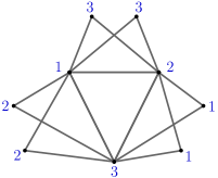
Figure 1: An illustrative example for MSCP [23]. The optimal coloring of the graph leads to an upper bound of the chromatic sum of the graph.

As shown in [42], MSCP can be conveniently formulated as an integer linear programming problem as follows:

$$\begin{array}[]{ll}\textrm{minimize}&g(x)=\sum_{i=1}^{n}\sum_{l=1}^{k}l\cdot x_{il}\\ \textrm{subject to}&\left\{\begin{array}[]{l}\sum_{l=1}^{k}x_{il}=1,i\in\{{1,\ldots,n}\}\\ x_{il}+x_{jl}\leq 1,\forall\{v_{i},v_{j}\}\in E,l\in\{{1,\ldots,k}\}\\ x_{il}\in\{{0,1}\}\end{array}\right.\end{array}$$ (3)

where $x_{il}=1$ ($i\in\{1,\ldots,n\},l\in\{1,\ldots,k\}$) if $v_{i}$ is assigned color $l$, $x_{il}=0$ otherwise.

The first constraint of this ILP model ensures that each vertex receives a single color while the second constraint states that two adjacent vertices cannot be assigned the same color. This linear model can be solved by any ILP solver like CPLEX [45]. Finally, as shown in [45], MSCP can also be formulated as a binary quadratic programming model.

3 Polynomial-time and $k$-approximation algorithms for MSCP

One notes that till now no exact algorithm especially designed for MSCP was reported in the literature except the general solution approach used in [45] which applies CPLEX to the integer linear programming formulation (Eq. (3)). On the other hand, a number of polynomial-time and $k$-approximation algorithms have been proposed for specific classes of graphs, such as trees, interval graphs, bipartite graphs, etc [9, 16, 22, 27, 36]. These algorithms exploit particular properties of the special graphs considered. In what follows, we briefly recall the main characteristics of these specific classes of graphs:

• A cograph, also called $P_{4}$-free graph, is a graph that does not contain the path $P_{4}$ for any four vertices;

• $P_{4}$-reducible graphs are a generalization of cographs where every vertex belongs to at most one $P_{4}$;

• $P_{4}$-sparse graphs generalize $P_{4}$-reducible graphs by imposing that every set of five vertices induces at most one $P_{4}$;

• Unicyclic graphs contain exactly one cycle;

• A partial $k$-tree $G$ is a graph with treewidth of at most $k$, where the treewidth is the size of the largest vertex set in a tree decomposition of $G$;

• A graph is outerplanar if it is planar (it can be embedded in the plane without crossing edges) and all its vertices lie on the exterior face;

• The line graph $L(G)$ of any graph $G=(V,E)$ is such that its vertex set is $E$ and two vertices of $L(G)$ are adjacent if their corresponding edges in $G$ are incident;

• In an interval graph, each vertex corresponds to an interval (over the set of real numbers for instance) and there is an edge between two vertices if their corresponding intervals intersect.

In the field of VLSI design, Kroon et al. [28] considered the “optimum cost chromatic partition problem” (OCCP), whose definition is similar to MSCP. For this problem, they introduced a linear-time algorithm for trees (see also [33]). Other classes of graph optimally solved in linear time include cographs [21] or unicyclic graphs [31] for instance.

In [21], Jansen found that the OCCP can be solved in polynomial time for partial $k$-trees. Then, Salavatipour presented a polynomial-time algorithm for $P_{4}$-reducible graphs [41]. Furthermore, Bonomo and Valencia-Pabon studied $P_{4}$-sparse graphs and found a large sub-family of $P_{4}$-sparse graphs that can be solved in polynomial time [7]. A cubic algorithm has also been proposed for outerplanar graphs [31].

Bar-Noy et al. proposed a 2-approximation algorithm for line graphs and showed a $(\Delta+2)/3$-approximation algorithm for graphs with maximum degree $\Delta$ [1]. Then, Bar-Noy and Kortsarz proposed a 10/9-approximation algorithm for bipartite graphs [3]. This approximation ratio was next improved to 27/26 by Malafiejski et al. [37] which is the best ratio for bipartite graphs to our knowledge. For interval graphs, Nicoloso et al. presented a 2-approximation algorithm [40], the best known ratio for this class of graphs being 1.796 [17]. Let us finally mention a 2-approximation algorithm for the entire class of $P_{4}$-sparse graphs [6].

4 Heuristics and metaheuristics for MSCP

Since these approximability results cannot be generalized to an arbitrary graph, for practically solving MSCP in the general case, a number of heuristic and metaheuristic algorithms have been proposed recently. In this section, we review the most representative and effective MSCP heuristic and metaheuristic algorithms which belong to three large classes of methods: greedy algorithms, local search heuristics, and evolutionary algorithms. For each reviewed algorithm, we identify its key ingredients, and highlight if the search process is constrained in the feasible space or is allowed to visit infeasible regions. We also provide in Table 1 a summary of the reviewed algorithms as well as indicators about their performances.

4.1 Greedy algorithms

Greedy algorithms are among the first heuristics proposed for MSCP. These algorithms are generally fast, simple, and easy to implement. Nevertheless, they usually achieve results of poor quality. On the other hand, given their particular features (speed and simplicity), they can advantageously be integrated into other more elaborated approaches where the greedy heuristic is used to generate an initial solution and seeds the search process. For instance, they can be used to provide initial upper bounds for an exact algorithm or to build the initial solution(s) for local search heuristics and evolutionary algorithms.

Two families of greedy algorithms for MSCP are proposed in [35]: MDSAT(n) and MRLF(n). They are based on the two well-known greedy coloring heuristics DSATUR [10] and RLF [34].

The original DSATUR heuristic employs the saturation degree $dsat$ of a vertex as the selection criterion to dynamically determine the next vertex to color. MDSAT(n) improves DSATUR by considering the impact of coloring a vertex where the impact is measured based on the number of vertices whose $dsat$ would (not) be changed. The original RLF heuristic follows the partition perspective of a vertex coloring. It colors as many non-adjacent vertices as possible with one color before going to another color. MRLF(n) which extends RLF is based on the idea of selecting the next candidate vertex $v$ for coloring such that it reduces the chance of using a new color next and keeps the current color class as large as possible. To achieve this goal, MRLF(n) implements sophistic greedy rules which rely on the cardinality of a subset of uncolored vertices that could be colored with and without using a new color.

A more complicated greedy heuristic (EXSCOL) is proposed in [46, 48]. It is based on independent set extraction and is highly effective for hard and large graphs. At each iteration, EXSCOL first identifies an independent set $S$ as large as possible by using a tabu search procedure. Secondly, it searches as many independent sets as possible of the same size $|S|$ to build a pool of candidate independent sets. Then, EXSCOL determines a maximum number of disjoint independent sets by solving a maximum set packing problem. Finally, the vertices of each extracted independent set receive the same smallest available color to form a color class. The above process is repeated until the graph becomes empty. Notice that there is no procedure to reconsider the extracted independent sets such that it is impossible for EXSCOL to attain an optimal solution once a “bad” independent set has been extracted.

4.2 Local search heuristics

Local search (or neighborhood search) heuristics progressively modify a candidate solution $c$ by local transformations until a stop condition is reached [15]. The two key components of a local search procedure are the evaluation function and the move (or transformation) operator which are defined on a given search space.

The evaluation function is used to assess the quality of a given coloring. The existing MSCP algorithms employ one of two types of evaluation function according to whether feasible or infeasible colorings are visited. For algorithms that explore only feasible solutions (i.e. proper colorings), the minimization function $f$ (i.e., the sum of colors, Eq. (1)) of the MSCP problem is directly used. On the other hand, algorithms that visit both feasible and infeasible solutions usually call for an augmented evaluation function $f_{p}$ which combines the objective function $f$ and a penalty function $p$.

In local search algorithms, one iteratively uses one or more move operators to transform the incumbent solutions $c$ to generate new neighboring solutions $c^{\prime}$. The set of neighboring solutions that can be reached by applying a move operator ($mv$) to the current solution forms the neighborhood (denoted by $N_{mv}$). We describe the commonly used operators as follows.

• One-move changes the color of a vertex in the current solution by moving a vertex $v$ from its current color class $V_{i}$ to another color class $V_{j}$ ($i\neq j$). This operator can generate both proper or improper colorings and thus can be used to explore feasible and infeasible regions of the coloring search space;

• Swap displaces a vertex $v$ from its current color class $V_{i}$ to another color class $V_{j}$ (as One-move) and then moves all adjacent vertices $u$ of $v$ to $V_{i}$. This operator can generate both proper or improper colorings;

• Exchange swaps a subset of vertices $A\subset V_{i}$ ($|A|>1$) and another subset of vertices $B\subset V_{j}$ ($|B|>1$) ($i\neq j$) such that the subgraph induced by $A\cup B$ is a connected component [24]. The new solution $c^{\prime}$ is feasible (respectively infeasible) if the starting solution $c$ is feasible (infeasible).

In what follows, we classify the representative local search algorithms into two categories according to the adopted neighborhood(s): single neighborhood search and multi-neighborhood search. Since local search can get stuck in local optima, most local search algorithms for MSCP use some diversification techniques to help the search to escape local optima encountered during the search. This is typically achieved by applying one or more perturbation operators to change a local optimum in a random or dedicated way.

4.2.1 Single neighborhood search

The tabu search (TS) algorithm proposed in [8] adapts the tabu algorithm designed for the classic vertex coloring problem [13, 20]. It starts with a random coloring and visits both proper and improper colorings with the neighborhood $N_{One-move}$ induced by the One-move operator. If there exist conflicting vertices, TS chooses a best move (according to its evaluation function $f_{p}$) to change the color of a conflicting vertex. Otherwise, TS picks a (non-conflicting) vertex and change its color at random. The above steps are repeated until a stopping criterion is satisfied. This algorithm relies simply on the tabu list for its diversification and does not call for other perturbation mechanism. This algorithm only showed limited computational results.

The breakout local search (BLS) algorithm described in [4] jointly uses two descent methods and an adaptive multi-perturbation strategy to escape local optima. The basic idea of BLS is to use descent-based local search to discover local optima and employ adaptive perturbations to continually visit different search regions in the search space. BLS explores both feasible and infeasible solutions with the help of the One-move operator. At each iteration, if the current solution $c$ is a feasible coloring, BLS applies a first descent search procedure to attain a local optimum in terms of the objective function $f$. If $c$ is an infeasible coloring (i.e., with conflicting vertices), BLS applies another descent search procedure guided by an augmented evaluation function which takes into account both the objective function $f$ and the conflicting vertices. BLS is characterized by its adaptive perturbation strategy which, upon the discover of a local optimum, triggers dedicated perturbation operations to escape the local optimum trap. Based on the information on the search state, the perturbation strategy of BLS introduces a varying degree of diversification by dynamically determining the number of perturbation moves to be applied and by adaptively selecting the suitable moves (random or directed perturbations).

4.2.2 Multi-neighborhood search

The MDS(5)+LS algorithm [19] applies an iterated multi-neighborhood search and also explores feasible and infeasible regions of the search space. It first employs the Swap operator until no further improvement exists in terms of its augmented evaluation function. Note that the obtained solution is not necessarily a proper coloring. If this is the case, MDS(5)+LS switches then to the One-move operator to repair the solution. Additional colors can be used to guarantee that the final coloring is proper at the end of this search phase. Finally, it assigns all the vertices with their smallest legal color and changes the color labels according to the sorted cardinality of the color classes $V_{l}$ ($|V_{1}|\geq\ldots\geq|V_{k}|$). Afterward, a random perturbation operator is applied which consists in moving some vertices from their current color class to another color class at random. This perturbed solution is then used as the starting point of the next round of the search procedure.

Table 1: Main heuristic and metaheuristic algorithms for MSCP

Algorithm name	Reference	Type of approach	Neighborhoods	Perturbation	Comments on performance
MDSAT(n) MRLF(n)	[35](2009)	Greedy search	-	-	A family of improved greedy algorithms based on the well-known greedy coloring strategies DSATUR and RLF.
TS	[8](2010)	Local search	$N_{One-move}$	No	A very simple tabu search but the results are better than those of the greedy algorithms MDSAT(n) and MRLF(n).
MDS(5)+LS	[19](2011)	Local search	$N_{One-move}$ $\&$ $N_{Swap}$	Yes	An iterated multi-neighborhood search combined with a random perturbation procedure achieving better results than MDSAT(n), MRLF(n) and TS.
BLS	[4](2012)	Local search	$N_{One-move}$	Yes	A breakout local search combining a greedy descent strategy with an adaptive perturbation step. It performs well on the small DIMACS graphs.
EXSCOL	[46, 48](2012)	Greedy + tabu search	No	No	A complicated greedy algorithm, based on independent sets extraction with tabu search, which is quite effective for large graphs.
MASC	[24](2014)	Evolutionary search	$N_{One-move}$ & $N_{Exchange}$	Yes	A memetic algorithm based on a double-neighborhood tabu search and a multi-parent crossover operator. Most results are better than those of the neighborhood search heuristics.
MA-MSCP	[39](2013)	Evolutionary search	$N_{One-move}$	Yes	A genetic algorithm with a two-parents crossover operator combined with a local search based on a hill climbing and a “destroy & repair” procedures. Results are comparable to those of MASC.
HESA	[23](2016)	Evolutionary search	$N_{One-move}$	Yes	A hybrid search algorithm based on a jointly use of two crossover operators and an iterated double-phase tabu search procedure. The lower and upper bounds obtained by the HESA are highly competitive with the best known results in the literature.

4.3 Evolutionary algorithms

Different from local search algorithms which are based on a single solution, evolutionary algorithms use a pool of solutions and try to find gradually better solutions by applying genetic operators (e.g., crossover, mutation, …) to solutions of the population [15].

The most popular evolutionary algorithms for MSCP follow the hybrid evolution framework called the memetic algorithm which jointly uses a recombination operator and a local search improvement to explore the search space [15]. They include, for instance, the MASC algorithm [24], MA-MSCP algorithm [39] and the HESA hybrid search algorithm [23]. Besides, an early parallel genetic algorithm PGA [26] employs assignment and partition crossovers, first-fit mutation, and proportional selection without any local search improvement.

The MASC memetic algorithm [24] follows the design guidelines of memetic algorithms for discrete optimization [18] and combines a multi-parent crossover operator (called MGPX) and a double-neighborhood tabu search procedure. MGPX is a variant of the well-known GPX crossover originally proposed for the classical vertex coloring problem [13]. It builds the color classes of the offspring (which is always a proper coloring) one by one and transmits entire color classes as large as possible until all vertices of the offspring are colored. Besides, the tabu search procedure applies the two different and complementary neighborhoods induced by Exchange and One-move in a token-ring way to find good local optima (according to the objective function $f$) until the search is stagnating. MASC employs a dedicated perturbation operator to diversify the search. MASC only explores the feasible search space of MSCP.

MA-MSCP is another hybrid genetic algorithm [39] that also focuses on the feasible search space. It includes a two-parent crossover operator (yet another adaptive variant of GPX [13]), a hill-climbing local search algorithm and a “destroy & repair” procedures. During the local search phase, the hill-climbing procedure is first applied to improve the current solution by using the One-move operator. To escape local optima, MA-MSCP then applies the “destroy & repair” strategy, which randomly removes some vertices and re-inserts each of them into its largest available color class while keeping the solution feasible. If there is no such a color class, the vertex is moved to a new color class. MA-MSCP employs the above two procedures alternately until no further improvement can be obtained.

HESA is also a hybrid search algorithm [23] that alternates between feasible and infeasible regions of the search space. HESA relies on a double-crossover recombination method and an iterated double-phase tabu search procedure. The recombination method jointly uses a diversification-guided crossover and a grouping-guided crossover to generate promising offspring solutions. During the double-phase tabu search procedure, it first checks if the given solution $c$ is a proper coloring. If $c$ is proper, the first tabu search is called to improve its sum of colors. Otherwise, another tabu search is used to attain a proper coloring which is further improved by the first tabu search to obtain a better sum of colors. The double-phase tabu search only explores the $N_{\textrm{One-move}}$ neighborhood. For the purpose of search diversification, HESA applies a conditional mixed perturbation strategy: 1) apply the Swap operator to a randomly chosen vertex to transform the incumbent solution, or 2) replace the current solution by the last local optimum.

Table 1 summarizes the reviewed existing heuristic algorithms with their main characteristics including the type of search paradigm, the neighborhood(s) and the presence or absence of a perturbation strategy together with a comment on their relative performance.

Finally, we mention the BQP-PR evolutionary algorithm [45] which relies on a binary quadratic programming formulation of the problem (see Section 2) and combines a path relinking approach with a tabu search procedure.

5 Bounds for MSCP

We will refer here to “theoretical” (lower and upper) bounds if they are formally proved, see Section 5.1. By opposition, “computational” bounds introduced in Section 5.2 designate those obtained running approximate algorithms.

5.1 Theoretical bounds

Recall that for any undirected simple graph $G=(V,E)$ with $n=|V|$ vertices and $m=|E|$ edges, the chromatic number $\chi(G)$ is the smallest number of colors needed to color the vertices of $G$ such that a proper $k$-coloring exists and the chromatic sum $\sum(G)$ is the minimum sum of the colors assigned to all vertices among all proper $k$-colorings of $G$. In this section, we list the current known theoretical lower and upper bounds of MSCP according to [26, 39, 44].

$$\begin{split}&\sum(G)\leq n+m\\ &\lceil{\sqrt{8m}}\rceil\leq\sum(G)\leq\lfloor\frac{3(m+1)}{2}\rfloor\\ &n+\frac{\chi(G)(\chi(G)-1)}{2}\leq\sum(G)\leq\lfloor\frac{n(\chi(G)+1)}{2}\rfloor\end{split}$$ (4)

From Eq.(4), one easily observes that the best theoretical lower and upper bounds available for MSCP are respectively $LB_{t}=\max\{\lceil{\sqrt{8m}}\rceil,n+\frac{\chi(G)(\chi(G)-1)}{2}\}$ and $UB_{t}=\min\{n+m,\lfloor\frac{3(m+1)}{2}\rfloor,\lfloor\frac{n(\chi(G)+1)}{2}\rfloor\}$.

5.2 Computational bounds

Given that MSCP is to find a proper $k$-coloring while minimizing the sum of the colors assigned to the vertices, Eq. (1) gives a computational upper bound for MSCP.

Let $G^{\prime}=(V,E^{\prime})(E^{\prime}\subseteq E)$ be any partial graph of $G=(V,E)$, $\sum(G^{\prime})$ is a lower bound of $\sum(G)$ since any proper coloring of $G$ must be a proper coloring of $G^{\prime}$: $\sum(G)\geq\sum(G^{\prime})$.

Partial graphs considered in the literature to estimate the computational lower bound $f_{LB}$ include bipartite graphs (trees and paths) [14, 28] and cliques [38, 48], while graph decomposition into cliques provide better bounds according to [38]. Let $c=\{S_{1},S_{2},$ $\ldots,S_{k}\}$ be a clique decomposition of $G$, then Eq. (5) gives a computational lower bound for MSCP since there is a single way of coloring any clique $S_{l}$ (with $|S_{l}|$ colors) and the sum of colors of $S_{l}$ is $|S_{l}|(|S_{l}|+1)/2$.

$$f_{LB}(c)=\sum_{l=1}^{k}\frac{|S_{l}|(|S_{l}|+1)}{2}$$ (5)

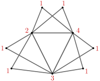
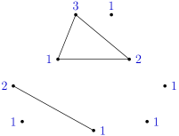
Figure 2: An illustrative lower bound via clique decomposition. The right figure is a clique decomposition of the graph on the left.

Figure 2 shows an illustrative lower bound via clique decomposition. We decompose $G$ into six cliques by ignoring some edges of the original graph $G$ and obtain the chromatic sum $\sum(G^{\prime})=13$ (right figure). Clearly, this is a lower bound for MSCP while the chromatic sum $\sum(G)=15$ (left figure).

To obtain a clique decomposition, one popular approach is to find a proper coloring of the complementary graph $\bar{G}$ of $G$ [19, 23, 39, 48], since each color class of $\bar{G}$ is a clique of $G$.

6 Benchmark and performance evaluation

In this section, we first introduce a set of MSCP instances (benchmarks) that are commonly used to assess the performance of MSCP algorithms and then provide indications about the performances of the reviewed MSCP algorithms. Due to many different factors (programming languages, running platforms, experimental protocols…), it is quite difficult to draw definitive conclusions. Nevertheless, we try to provide some useful indications with respect to their performance in terms of best and average results.

6.1 Benchmark

There exists a set of 94 frequently used benchmark instances often used for performance evaluation of MSCP algorithms. 58 instances are part of the COLOR 2002–2004 competitions while the remaining 36 instances come from the second DIMACS challenge. Compared to the well-known DIMACS instances, the COLOR 2002-2004 instances are relatively easy except the four large “wap” graphs. These instances refer to various topologies and densities, which can be classified into the 13 following types:

• Twelve classical random graphs (DSJC$n.d,n\in\{125,250,500,1\,000\},d\in\{1,5,9\}$);

• Three geometric graphs (DSJR500.$d$, $d\in\{1c,1,5\}$);

• Six flat graphs (flat$300\_\chi\_0$ with $\chi\in\{20,26,28\}$ and flat$1000\_\chi\_0$ with $\chi\in\{50,60,76\}$);

• Twelve Leighton graphs (le450_$\chi$a, le450_$\chi$b, le450_$\chi$c, le450_$\chi$d, $\chi\in\{5,15,25\}$);

• Four latin square graph (latin_sqr_10 and qg.order$\chi$, $\chi\in\{30,40,50\}$);

• Two very large random graphs (C2000.5 and C4000.5);

• Fourteen graphs based on register allocation (fpsol2.i.$a$, inithx.i.$a$, zeroin.i.$a$, mulsol.i.$b$, $a\in\{1,2,3\}$ and $b\in\{1,2,3,4,5\}$);

• Two graphs from the scheduling area (school1 and school1_nsh);

• Twenty four graphs from the Donald Knuth’s Stanford GraphBase (miles$n$ with $n\in\{250,500,750,1000,1500\}$, anna, david, huck, jean, homer, games120, queen8.12, and queen$a.a$, $a\in\{5,\ldots,16\}$);

• Five graphs based on the Mycielski transformation (myciel$a$, $a\in\{3,4,5,6,7\}$);

• Four graphs that have a hard-to-find four clique embedded (mug$n\_a$, $n\in\{88,100\}$, $a\in\{1,25\}$);

• Two “insertion” graphs (2-Insert_3 and 3-Insert_3);

• Four graphs from real-life optical network design problems (wap05, wap06, wap07, and wap08).

Table 2: Main characteristics of MSCP benchmark (94 instances)

Graph $G$	$n$	$m$	$d$	$\chi(G)$	$LB_{t}$	$UB_{t}$	Graph $G$	$n$	$m$	$d$	$\chi(G)$	$LB_{t}$	$UB_{t}$
myciel3	11	20	0.36	4	17	27	zeroin.i.1	211	4100	0.19	49	1387	4311
myciel4	23	71	0.28	5	33	69	zeroin.i.2	211	3541	0.16	30	646	3270
myciel5	47	236	0.22	6	62	164	zeroin.i.3	206	3540	0.17	30	641	3193
myciel6	95	755	0.17	7	116	380	wap05	905	43081	0.11	50	2130	23077
myciel7	191	2360	0.13	8	219	859	wap06	947	43571	0.10	40	1727	19413
anna	138	493	0.05	11	193	631	wap07	1809	103368	0.06	$\leq 41$	2629	37989
david	87	406	0.11	11	142	493	wap08	1870	104176	0.06	$\leq 42$	2731	40205
huck	74	301	0.11	11	129	375	qg.order30	900	26100	0.06	30	1335	13950
jean	80	254	0.08	10	125	334	qg.order40	1600	62400	0.05	40	2380	32800
homer	561	1628	0.01	13	639	2189	qg.order60	3600	212400	0.03	60	5370	109800
queen5.5	25	160	0.53	5	36	75	DSJC125.1	125	736	0.09	5	135	375
queen6.6	36	290	0.46	7	57	144	DSJC125.5	125	3891	0.50	17	261	1125
queen7.7	49	476	0.40	7	70	196	DSJC125.9	125	6961	0.90	44	1071	2812
queen8.8	64	728	0.36	9	100	320	DSJC250.1	250	3218	0.10	$\leq 8$	278	1125
queen8.12	96	1368	0.30	12	162	624	DSJC250.5	250	15668	0.50	$\leq 28$	628	3625
queen9.9	81	1056	0.33	10	126	445	DSJC250.9	250	27897	0.90	$\leq 72$	2806	9125
queen10.10	100	1470	0.30	11	155	600	DSJC500.1	500	12458	0.10	$\leq 12$	566	3250
queen11.11	121	1980	0.27	11	178	726	DSJC500.5	500	62624	0.50	$\leq 47$	1581	12000
queen12.12	144	2596	0.25	12	210	936	DSJC500.9	500	112437	0.90	$\leq 126$	8375	31750
queen13.13	169	3328	0.23	13	247	1183	DSJC1000.1	1000	49629	0.10	$\leq 20$	1190	10500
queen14.14	196	4186	0.22	14	287	1470	DSJC1000.5	1000	249826	0.50	$\leq 82$	4321	41500
queen15.15	225	5180	0.21	15	330	1800	DSJC1000.9	1000	449449	0.90	$\leq 222$	25531	111500
queen16.16	256	6320	0.19	16	376	2176	DSJR500.1	500	3555	0.03	12	566	3250
school1	385	19095	0.26	14	476	2887	DSJR500.1c	500	121275	0.97	84	3986	21250
school1-nsh	352	14612	0.24	14	443	2640	DSJR500.5	500	58862	0.47	122	7881	30750
miles250	128	387	0.05	8	156	515	flat300_20_0	300	21375	0.48	20	490	3150
miles500	128	1170	0.14	20	318	1298	flat300_26_0	300	21633	0.48	26	625	4050
miles750	128	2113	0.26	31	593	2048	flat300_28_0	300	21695	0.48	28	678	4350
miles1000	128	3216	0.40	42	989	2752	flat1000_50_0	1000	245000	0.49	50	2225	25500
miles1500	128	5198	0.64	73	2756	4736	flat1000_60_0	1000	245830	0.49	60	2770	30500
fpsol2.i.1	496	11654	0.09	65	2576	12150	flat1000_76_0	1000	246708	0.49	76	3850	38500
fpsol2.i.2	451	8691	0.09	30	886	6990	le450_5a	450	5714	0.06	5	460	1350
fpsol2.i.3	425	8688	0.10	30	860	6587	le450_5b	450	5734	0.06	5	460	1350
mug88_1	88	146	0.04	4	94	220	le450_5c	450	9803	0.10	5	460	1350
mug88_25	88	146	0.04	4	94	220	le450_5d	450	9757	0.10	5	460	1350
mug100_1	100	166	0.03	4	106	250	le450_15a	450	8168	0.08	15	555	3600
mug100_25	100	166	0.03	4	106	250	le450_15b	450	8169	0.08	15	555	3600
2-Insert_3	37	72	0.11	4	43	92	le450_15c	450	16680	0.17	15	555	3600
3-Insert_3	56	110	0.07	4	62	140	le450_15d	450	16750	0.17	15	555	3600
inithx.i.1	864	18707	0.05	54	2295	19571	le450_25a	450	8260	0.08	25	750	5850
inithx.i.2	645	13979	0.07	31	1110	10320	le450_25b	450	8263	0.08	25	750	5850
inithx.i.3	621	13969	0.07	31	1086	9936	le450_25c	450	17343	0.17	25	750	5850
mulsol.i.1	197	3925	0.20	49	1373	4122	le450_25d	450	17425	0.17	25	750	5850
mulsol.i.2	188	3885	0.22	31	653	3008	latin_sqr_10	900	307350	0.76	$\leq 97$	5556	44100
mulsol.i.3	184	3916	0.23	31	649	2944	C2000.5	2000	999836	0.50	$\leq 145$	12585	147000
mulsol.i.4	185	3946	0.23	31	650	2960	C4000.5	4000	4000268	0.50	$\leq 259$	37670	522000
mulsol.i.5	186	3973	0.23	31	651	2976	games120	120	638	0.09	9	156	600

Table 2 gives the detailed characteristics of the benchmark graphs. Columns 2–5 and 9–12 indicate the number $n$ of vertices, the number $m$ of edges, the density $d=2m/n(n-1)$ and the chromatic number $\chi(G)$ of each graph. Columns 6–7 and 13–14 show the best theoretical lower and upper bounds of the chromatic sum ($LB_{t}$ and $UB_{t}$ respectively). Underlined entries (in all tables) indicate that theoretical upper bounds equal the computational upper bounds while no theoretical lower bound equals the computational lower bound. Note that, since the chromatic number $\chi(G)$ of some difficult graphs are still unknown, we use the minimum $k$ for which a $k$-coloring has been reported for $G$ in the literature instead of $\chi(G)$ to compute $LB_{t}$ and $UB_{t}$ using the $\min/\max$ equations introduced in Section 5.1.

6.2 Performance of MSCP algorithms

Based on the benchmark introduced in the previous section, Table LABEL:table_many_algorithms (see the Appendix) summarizes the computational results of six representative and effective MSCP algorithms presented in Section 4: BLS [4], MASC [24], MDS(5)+LS [19], EXSCOL [46, 48], MA-MSCP [39] and HESA [23]. Columns 1–3 present the tested graph and its best known lower and upper bounds ($f^{b}_{LB}$ and $f^{b}_{UB}$ respectively, in bold face when optimality is proved), the following 18 columns give the detailed computational results of the six algorithms. “–” marks for the reference algorithms mean non-available results. The results in terms of solution quality (best / average lower and upper bounds, $f^{*}_{LB}/f^{a}_{LB}$ and $f^{*}_{UB}/f^{a}_{UB}$ respectively) are directly extracted from the original papers. Computing times are not listed in the table due to the difference of experimental conditions (platforms, programming languages, stop conditions…). Nevertheless, the second and third lines of the heading respectively indicate the main computer characteristic (processor frequency) and the stop condition to have an idea of the maximum amount of search used by each approach. Note that there is no specific stop condition for EXSCOL since its extraction process ends when the current graph becomes empty. Furthermore, some heuristics can halt before reaching the stop criterion, when a known (lower) bound is reached for instance.

From Table LABEL:table_many_algorithms, one observes that only HESA reports results for all the 94 graphs of the benchmark. Besides, MDS(5)+LS, EXSCOL, MA-MSCP, and HESA provide lower and upper bounds while BLS and MASC only give an upper bound. Additionally, Figure 3 provides performance information of each of the six algorithms compared to the best known upper and lower bounds. One observes that no algorithm can reach all the best known results. BLS and MASC attain the best upper bounds for 17 graphs out of the 27 tested graphs and for 56 graphs out of the 77 tested graphs respectively. MDS(5)+LS reaches the best lower (upper) bound for 24 (26) instances out of 38. EXSCOL reaches the best lower and upper bounds for 38 (out of 62 graphs) and 24 (out of 52 graphs) respectively. MA-MSCP reaches the best lower / upper bound for 51 / 53 graphs out of 81. HESA equals the best lower (upper) bound for 86 (85) instances out of 94.

Since the number of tested graphs differs from one algorithm to another, the performance of these algorithms cannot be compared from a statistical viewpoint. However, from Table LABEL:table_many_algorithms and Figure 3, we can roughly conclude that BLS, MASC, MDS(5)+LS, EXSCOL, MA-MSCP and HESA are currently the most effective algorithms for solving the MSCP problem.

From the theoretical and computational bounds reviewed above, we can make the following observations:

• Optimality is proved for 21 instances out of the 94 tested graphs since the best upper bounds are equal to the best lower bounds (see entries in bold in Table LABEL:table_many_algorithms);

• 12 theoretical upper bounds equal the computational upper bounds while no theoretical lower bound equals the computational lower bound (underlined in Tables 2–LABEL:table_many_algorithms);

• The theoretical upper bounds of queen$a.a~{}(a\in\{11,12,13,14,15,16\})$ are equal to the best computational lower bounds meaning optimal results;

• Table LABEL:table_many_algorithms shows that the best computational lower bounds of some easy graphs (myciel$a$, $a\in\{3,4,5,6\}$, for instance) are not equal to the optimal upper bounds (optimality proved with CPLEX [45]). Hence, the method of decomposing the graph introduced in Section 5.2 is not good enough in some cases and should be improved.

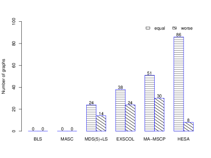
(a) Lower bounds

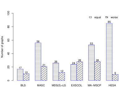
(b) Upper bounds

Figure 3: The performance of six representative MSCP algorithms. The y-axis shows the number of graphs for which an algorithm attains a result equal to or worse than the best known reported bound.

7 Perspectives and conclusion

This review is dedicated to recent approximation algorithms and practical solution algorithms designed for the minimum sum coloring problem which attracted increasing attention in recent years. MSCP is a strongly constrained combinatorial optimization problem which is theoretically important and computationally difficult. In addition to its relevance as a typical model to formulate a number of practical problems, MSCP can be used as a benchmark problem to test constraint satisfaction algorithms and solvers.

Based on this review, we discuss some perspective research directions.

• Evaluation function and search space: as introduced in Section 2, the aim of MSCP is twofold: (1) find a proper $k$-coloring $c$ of a graph and (2) ensure that the sum of the colors assigned to the vertices is minimized. An evaluation function combining these two objectives has been proposed in [19]:

  $$f^{\prime}(c)=\sum_{l=1}^{k}l|V_{l}|+M|E(V_{l})|$$

  where $E(V_{l})$ is the set of conflicting edges in $V_{l}$ and $M>0$ is a sufficiently large natural number. Since the evaluation function is used to guide the heuristic search process, it would be interesting to design other effective evaluation function based on a better recombination of the two parts of $f^{\prime}$.

  Another possibility could be to explore only the feasible graph coloring search space, like in the competitive MASC and MA-MSCP approaches [24, 39], using more effective (multi-)neighborhood structures.

  Besides, the combination of the above two ingredients in a proper way may lead to improved MSCP algorithms.

• Maximum independent sets extraction: As shown in Section 4.1, EXSCOL is a greedy heuristic based on the independent sets extraction that is quite effective for large graphs. Its major deficiency is that it does not include a procedure to reconsider “bad” independent sets that has been extracted. Hence, one possibility is to devise a backtracking procedure when a “bad” independent set has been identified as proposed for the graph coloring problem [47].

• Exact algorithms: There is no exact algorithm especially designed for MSCP except the general approach which applies CPLEX to solve the integer linear programming formulation of MSCP [45]. However, as shown in [45], this approach is only applicable to easy DIMACS instances. On the other hand, some exact algorithms for the classical vertex coloring problem successfully solved a subset of the hard DIMACS graphs. Hence, it would be important to fill the gap by designing exact algorithms for MSCP.

To conclude, the minimum sum coloring problem, like the classical coloring problem, is a generic and useful model. Advances in solution methods (both exact and heuristic methods) for these coloring problems will help find satisfying solutions to many practical problems. Given the increasing interest in the sum coloring problem and their related coloring problems, it is reasonable to believe that research in these domains will become even more intense and fruitful in the forthcoming years.

Appendix

For the purpose of completeness, this Appendix, which reproduces and extends the results given in [23], shows a performance summary of the six main heuristic algorithms for the set of 94 DIMACS benchmark graphs in terms of the lower and upper bounds of the MSCP problem.

Table 3: The performance of six heuristics and metaheuristics for the lower and upper bounds of MSCP

Graph				BLS [4]			MASC [24]			MDS(5)+LS [19]			EXSCOL [46, 48]					MA-MSCP [39]					HESA [23]
				2.83 GHz			2.7 GHz			2.93 GHz			2.8 GHz, 2.83 GHz					1.66 GHz					2.83 GHz
				2 hours			50 generations			1 hour			No stop condition					2 hours					2 hours
Name	$f^{b}_{LB}$	$f^{b}_{UB}$		$f^{*}_{UB}$	$f^{a}_{UB}$		$f^{*}_{UB}$	$f^{a}_{UB}$		$f^{*}_{LB}$	$f^{*}_{UB}$		$f^{*}_{LB}$	$f^{a}_{LB}$	$f^{*}_{UB}$	$f^{a}_{UB}$		$f^{*}_{LB}$	$f^{a}_{LB}$	$f^{*}_{UB}$	$f^{a}_{UB}$		$f^{*}_{LB}$	$f^{a}_{LB}$	$f^{*}_{UB}$	$f^{a}_{UB}$
myciel3	16	21		21	21.0		21	21.0		16	21		16	16.0	21	21.0		16	16.0	21	21.0		16	16.0	21	21.0
myciel4	34	45		45	45.0		45	45.0		34	45		34	34.0	45	45.0		34	34.0	45	45.0		34	34.0	45	45.0
myciel5	70	93		93	93.0		93	93.0		70	93		70	70.0	93	93.0		70	70.0	93	93.0		70	70.0	93	93.0
myciel6	142	189		189	196.6		189	189.0		142	189		142	142.0	189	189.0		142	139.5	189	189.0		142	142.0	189	189.0
myciel7	286	381		381	393.8		381	381.0		286	381		286	286.0	381	381.0		286	277.5	381	381.0		286	286.0	381	381.0
anna	273	276		276	276.0		276	276.0		273	276		273	273.0	283	283.2		273	273.0	276	276.0		273	273.0	276	276.0
david	234	237		237	237.0		237	237.0		234	237		229	229.0	237	238.1		234	234.0	237	237.0		234	234.0	237	237.0
huck	243	243		243	243.0		243	243.0		243	243		243	243.0	243	243.8		243	243.0	243	243.0		243	243.0	243	243.0
jean	216	217		217	217.0		217	217.0		216	217		216	216.0	217	217.3		216	216.0	217	217.0		216	216.0	217	217.0
homer	1129	1150		-	-		1155	1158.5		-	-		-	-	-	-		1129	1129.0	1157	1481.9		1129	1129.0	1150	1151.8
queen5.5	75	75		75	75.0		75	75.0		75	75		75	75.0	75	75.0		75	75.0	75	75.0		75	75.0	75	75.0
queen6.6	126	138		138	138.0		138	138.0		126	138		126	126.0	150	150.0		126	126.0	138	138.0		126	126.0	138	138.0
queen7.7	196	196		196	196.0		196	196.0		196	196		196	196.0	196	196.0		196	196.0	196	196.0		196	196.0	196	196.0
queen8.8	288	291		291	291.0		291	291.0		288	291		288	288.0	291	291.0		288	288.0	291	291.0		288	288.0	291	291.0
queen8.12	624	624		-	-		624	624.0		-	-		-	-	-	-		624	624.0	624	624.0		624	624.0	624	624.0
queen9.9	405	409		-	-		409	410.5		-	-		-	-	-	-		405	405.0	409	411.9		405	405.0	409	409.0
queen10.10	550	553		-	-		-	-		-	-		-	-	-	-		550	550.0	553	555.2		550	550.0	553	553.6
queen11.11	726	733		-	-		-	-		-	-		-	-	-	-		726	726.0	733	735.4		726	726.0	733	734.4
queen12.12	936	943		-	-		-	-		-	-		-	-	-	-		936	936.0	944	948.7		936	936.0	943	947.0
queen13.13	1183	1191		-	-		-	-		-	-		-	-	-	-		1183	1183.0	1192	1197.0		1183	1183.0	1191	1195.4
queen14.14	1470	1482		-	-		-	-		-	-		-	-	-	-		1470	1470.0	1482	1490.8		1470	1470.0	1482	1487.3
queen15.15	1800	1814		-	-		-	-		-	-		-	-	-	-		1800	1800.0	1814	1823.0		1800	1800.0	1814	1820.1
queen16.16	2176	2193		-	-		-	-		-	-		-	-	-	-		2176	2176.0	2197	2205.9		2176	2176.0	2193	2199.4
school1	2439	2674		-	-		-	-		-	-		-	-	-	-		2345	2283.3	2674	2766.8		2439	2418.9	2674	2674.0
school1-nsh	2176	2392		-	-		-	-		-	-		-	-	-	-		2106	2064.6	2392	2477.1		2176	2169.4	2392	2392.0
miles250	318	325		327	328.8		325	325.0		318	325		318	316.2	328	333.0		318	318.0	325	325.4		318	318.0	325	325.0
miles500	686	705		710	713.3		705	705.0		686	712		677	671.4	709	714.5		686	686.0	708	711.2		686	686.0	705	705.8
miles750	1145	1173		-	-		-	-		-	-		-	-	-	-		1145	1145.0	1173	1183.9		1145	1145.0	1173	1173.6
miles1000	1623	1666		-	-		-	-		-	-		-	-	-	-		1623	1623.0	1679	1697.3		1623	1623.0	1666	1670.5
miles1500	3239	3354		-	-		-	-		-	-		-	-	-	-		3239	3239.0	3354	3357.2		3239	3239.0	3354	3354.0
fpsol2.i.1	3403	3403		-	-		3403	3403.0		3151	3403		3403	3403.0	-	-		3403	3403.0	3403	3403.0		3403	3403.0	3403	3403.0
fpsol2.i.2	1668	1668		-	-		1668	1668.0		-	-		-	-	-	-		1668	1668.0	1668	1668.0		1668	1668.0	1668	1668.0
fpsol2.i.3	1636	1636		-	-		1636	1636.0		-	-		-	-	-	-		1636	1636.0	1636	1636.0		1636	1636.0	1636	1636.0
mug88_1	164	178		-	-		178	178.0		164	178		164	162.3	-	-		-	-	-	-		164	164.0	178	178.0
mug88_25	162	178		-	-		178	178.0		162	178		162	160.3	-	-		-	-	-	-		162	162.0	178	178.0
mug100_1	188	202		-	-		202	202.0		188	202		188	188.0	-	-		-	-	-	-		188	188.0	202	202.0
mug100_25	186	202		-	-		202	202.0		186	202		186	183.4	-	-		-	-	-	-		186	186.0	202	202.0
2-Insert_3	55	62		-	-		62	62.0		55	62		55	55.0	-	-		-	-	-	-		55	55.0	62	62.0
3-Insert_3	84	92		-	-		92	92.0		84	92		84	82.8	-	-		-	-	-	-		84	84.0	92	92.0
inithx.i.1	3676	3676		-	-		3676	3676.0		3486	3676		3676	3676.0	-	-		3676	3616.0	3676	3679.6		3676	3675.3	3676	3676.0
inithx.i.2	2050	2050		-	-		2050	2050.0		-	-		-	-	-	-		2050	1989.2	2050	2053.7		2050	2050.0	2050	2050.0
inithx.i.3	1986	1986		-	-		1986	1986.0		-	-		-	-	-	-		1986	1961.8	1986	1986.0		1986	1986.0	1986	1986.0
mulsol.i.1	1957	1957		-	-		1957	1957.0		-	-		-	-	-	-		1957	1957.0	1957	1957.0		1957	1957.0	1957	1957.0
mulsol.i.2	1191	1191		-	-		1191	1191.0		-	-		-	-	-	-		1191	1191.0	1191	1191.0		1191	1191.0	1191	1191.0
mulsol.i.3	1187	1187		-	-		1187	1187.0		-	-		-	-	-	-		1187	1187.0	1187	1187.0		1187	1187.0	1187	1187.0
mulsol.i.4	1189	1189		-	-		1189	1189.0		-	-		-	-	-	-		1189	1189.0	1189	1189.0		1189	1189.0	1189	1189.0
mulsol.i.5	1160	1160		-	-		1160	1160.0		-	-		-	-	-	-		1160	1160.0	1160	1160.0		1160	1160.0	1160	1160.0
zeroin.i.1	1822	1822		-	-		1822	1822.0		-	-		-	-	-	-		1822	1822.0	1822	1822.0		1822	1822.0	1822	1822.0
zeroin.i.2	1004	1004		-	-		1004	1004.0		1004	1004		1004	1004.0	-	-		1004	1002.1	1004	1004.0		1004	1004.0	1004	1004.0
zeroin.i.3	998	998		-	-		998	998.0		998	998		998	998.0	-	-		998	998.0	998	998.0		998	998.0	998	998.0
wap05	12449	13656		-	-		13669	13677.8		-	-		12428	12339.3	13680	13718.4		-	-	-	-		12449	12438.9	13656	13677.8
wap06	12454	13773		-	-		13776	13777.8		-	-		12393	12348.8	13778	13830.9		-	-	-	-		12454	12431.6	13773	13777.6
wap07	24800	28617		-	-		28617	28624.7		-	-		24339	24263.8	28629	28663.8		-	-	-	-		24800	24783.6	29154	29261.1
wap08	25283	28885		-	-		28885	28890.9		-	-		24791	24681.1	28896	28946.0		-	-	-	-		25283	25263.4	29460	29542.3
qg.order30	13950	13950		-	-		13950	13950.0		-	-		13950	13950.0	13950	13950.0		13950	13950.0	13950	13950.0		13950	13950.0	13950	13950.0
qg.order40	32800	32800		-	-		32800	32800.0		-	-		32800	32800.0	32800	32800.0		32800	32800.0	32800	32800.0		32800	32800.0	32800	32800.0
qg.order60	109800	109800		-	-		109800	109800.0		-	-		109800	109800.0	110925	110993.0		109800	109800.0	109800	109800.0		109800	109800.0	109800	109800.0
DSJC125.1	247	326		326	326.9		326	326.6		238	326		246	244.1	326	326.7		247	244.6	326	327.3		247	247.0	326	326.1
DSJC125.5	549	1012		1012	1012.9		1012	1020.0		493	1015		536	522.4	1017	1019.7		549	541.0	1013	1018.5		549	548.5	1012	1012.2
DSJC125.9	1691	2503		2503	2503.0		2503	2508.0		1621	2511		1664	1592.5	2512	2512.0		1689	1677.7	2503	2519.0		1691	1691.0	2503	2503.0
DSJC250.1	570	970		973	982.5		974	990.5		521	977		567	562.0	985	985.0		569	558.4	983	995.8		570	569.2	970	980.4
DSJC250.5	1287	3210		3219	3248.5		3230	3253.7		1128	3281		1270	1258.8	3246	3253.9		1280	1249.4	3214	3285.5		1287	1271.6	3210	3235.6
DSJC250.9	4311	8277		8290	8316.0		8280	8322.7		3779	8412		4179	4082.4	8286	8288.8		4279	4160.9	8277	8348.8		4311	4279.4	8277	8277.2
DSJC500.1	1250	2836		2882	2942.9		2841	2844.1		1143	2951		1250	1246.6	2850	2857.4		1241	1214.9	2897	2990.5		1250	1243.4	2836	2836.0
DSJC500.5	2923	10886		11187	11326.3		10897	10905.8		2565	11717		2921	2902.6	10910	10918.2		2868	2797.7	11082	11398.3		2923	2896.0	10886	10891.5
DSJC500.9	11053	29862		30097	30259.2		29896	29907.8		9731	30872		10881	10734.5	29912	29936.2		10759	10443.8	29995	30361.9		11053	10950.1	29862	29874.3
DSJC1000.1	2762	8991		9520	9630.1		8995	9000.5		2456	10123		2762	2758.6	9003	9017.9		2707	2651.2	9188	9667.1		2719	2707.6	8991	8996.5
DSJC1000.5	6708	37575		40661	41002.6		37594	37597.6		5660	43614		6708	6665.9	37598	37673.8		6534	6182.5	38421	40260.9		6582	6541.3	37575	37594.7
DSJC1000.9	26557	103445		-	-		103464	103464.0		23208	112749		26557	26300.3	103464	103531.0		26157	24572.0	105234	107349.0		26296	26150.3	103445	103463.3
DSJR500.1	2069	2156		-	-		-	-		-	-		-	-	-	-		2061	2052.9	2173	2253.1		2069	2069.0	2156	2170.7
DSJR500.1c	15398	16286		-	-		-	-		-	-		-	-	-	-		15025	14443.9	16311	16408.5		15398	15212.4	16286	16286.0
DSJR500.5	22974	25440		-	-		-	-		-	-		-	-	-	-		22728	22075.0	25630	26978.0		22974	22656.7	25440	25684.1
flat300_20_0	1531	3150		-	-		3150	3150.0		-	-		1524	1505.7	3150	3150.0		1515	1479.3	3150	3150.0		1531	1518.2	3150	3150.0
flat300_26_0	1548	3966		-	-		3966	3966.0		-	-		1525	1511.4	3966	3966.0		1536	1501.6	3966	3966.0		1548	1530.3	3966	3966.0
flat300_28_0	1547	4238		-	-		4238	4313.4		-	-		1532	1515.3	4282	4286.1		1541	1503.9	4261	4389.4		1547	1536.5	4260	4290.0
flat1000_50_0	6601	25500		-	-		25500	25500.0		-	-		6601	6571.8	25500	25500.0		6433	6121.5	25500	25500.0		6476	6452.1	25500	25500.0
flat1000_60_0	6640	30100		-	-		30100	30100.0		-	-		6640	6600.5	30100	30100.0		6402	6047.7	30100	30100.0		6491	6466.5	30100	30100.0
flat1000_76_0	6632	37164		-	-		37167	37167.0		-	-		6632	6583.2	37167	37213.2		6330	6074.6	38213	39722.7		6509	6482.8	37164	37165.9
le450_5a	1193	1350		-	-		1350	1350.0		-	-		-	-	-	-		1190	1171.5	1350	1350.0		1193	1191.5	1350	1350.0
le450_5b	1189	1350		-	-		1350	1350.0		-	-		-	-	-	-		1186	1166.5	1350	1350.0		1189	1185.0	1350	1350.1
le450_5c	1278	1350		-	-		1350	1350.0		-	-		-	-	-	-		1272	1242.3	1350	1350.0		1278	1270.4	1350	1350.0
le450_5d	1282	1350		-	-		1350	1350.0		-	-		-	-	-	-		1269	1245.2	1350	1350.0		1282	1274.2	1350	1350.0
le450_15a	2331	2632		-	-		2706	2742.6		-	-		2329	2313.7	2632	2641.9		2329	2324.3	2681	2733.1		2331	2331.0	2634	2648.4
le450_15b	2348	2632		-	-		2724	2756.2		-	-		2343	2315.7	2642	2643.4		2348	2335.0	2690	2730.6		2348	2348.0	2632	2656.5
le450_15c	2610	3487		-	-		3491	3491.0		-	-		2591	2545.3	3866	3868.9		2593	2569.1	3943	4048.4		2610	2606.6	3487	3792.4
le450_15d	2628	3505		-	-		3506	3511.8		-	-		2610	2572.4	3921	3928.5		2622	2587.2	3926	4032.4		2628	2627.1	3505	3883.1
le450_25a	3003	3153		-	-		3166	3176.8		-	-		2997	2964.4	3153	3159.4		3003	3000.4	3178	3204.3		3003	3003.0	3157	3166.7
le450_25b	3305	3365		-	-		3366	3375.1		-	-		3305	3304.1	3366	3371.9		3305	3304.1	3379	3416.2		3305	3305.0	3365	3375.2
le450_25c	3657	4515		-	-		4700	4773.3		-	-		3619	3597.1	4515	4525.4		3638	3617.0	4648	4700.7		3657	3656.9	4553	4583.8
le450_25d	3698	4544		-	-		4722	4805.7		-	-		3684	3627.4	4544	4550.0		3697	3683.2	4696	4740.3		3698	3698.0	4569	4607.6
latin_sqr_10	40950	41444		-	-		41444	41481.5		-	-		40950	40950.0	42223	42392.7		-	-	-	-		40950	40950.0	41492	41672.8
C2000.5	15091	132483		-	-		-	-		-	-		15091	15077.6	132515	132682.0		-	-	-	-		14498	14442.9	132483	132513.9
C4000.5	33033	473234		-	-		-	-		-	-		33033	33018.8	473234	473211.0		-	-	-	-		31525	31413.3	513457	514639.0
games120	442	443		443	443.0		443	443.0		442	443		442	441.4	443	447.9		442	442.0	443	443.0		442	442.0	443	443.0

References

- [1] Bar-Noy, A., Bellare, M., Halldórsson, M.M., Shachnai, H., Tamir, T. (1998). On chromatic sums and distributed resource allocation. Information and Computation 140, 183–202.
- [2] Bar-Noy, A., Halldórsson, M.M., Kortsarz, G., Salman, R., Shachnai, H. (1999). Sum multi-coloring of graphs. In: J. Nesetril (ed.), 7th Annual European Symposium on Algorithms, vol. 1643 of Lecture Notes in Computer Science, Springer, Berlin / Heidelberg, Germany, pp. 390–401.
- [3] Bar-Noy, A., Kortsarz, G. (1998). Minimum color sum of bipartite graphs. Journal of Algorithms 28(2): 339–365.
- [4] Benlic, U., Hao, J.-K. (2012). A study of breakout local search for the minimum sum coloring problem. In: L. Bui, Y. Ong, N. Hoai, H. Ishibuchi, P. Suganthan (eds.), Simulated Evolution and Learning, vol. 7673 of Lecture Notes in Computer Science, Springer, Berlin / Heidelberg, Germany, pp. 128–137.
- [5] Berliner, A., Bostelmann, U., Brualdi, R.A., Deaett, L. (2006). Sum list coloring graphs. Graphs and Combinatorics 22(2): 173–183.
- [6] Bonomo, F., Durán, G., Napoli, A., Valencia-Pabon, M. (2015). A one-to-one correspondence between potential solutions of the cluster deletion problem and the minimum sum coloring problem, and its application to -sparse graphs. Information Processing Letters 115(6–8): 600–603.
- [7] Bonomo, F., Valencia-Pabon, M. (2014). On the Minimum Sum Coloring of -sparse graphs. Graphs and Combinatorics 30(2): 303–314.
- [8] Bouziri, H., Jouini, M. (2010). A tabu search approach for the sum coloring problem. Electronic Notes in Discrete Mathematics 36: 915–922.
- [9] Borodin, A., Ivan, I., Ye, Y., Zimny, B. 2012. On sum coloring and sum multi-coloring for restricted families of graphs. Theoretical Computer Science 418: 1–13.
- [10] Brélaz, D. (1979). New methods to color the vertices of a graph. Communications of the ACM 22(4): 251–256.
- [11] Douiri, S., Elbernoussi, S. (2011). New algorithm for the sum coloring problem. International Journal of Contemporary Mathematical Sciences 6: 453–463.
- [12] Douiri, S., Elbernoussi, S. (2012). A new ant colony optimization algorithm for the lower bound of sum coloring problem. Journal of Mathematical Modelling and Algorithms 11(2): 181–192.
- [13] Galinier, P., Hao, J.-K. (1999). Hybrid evolutionary algorithms for graph coloring. Journal of Combinatorial Optimization 3(4): 379–397.
- [14] Garey, M.R., Johnson, D.S. (1979). Computers and intractability. A Guide to the Theory of NP-Completeness, Ed. Freeman and Company, New York.
- [15] Gendreau, M., Potvin ,J.Y. (2010). Handbook of metaheuristics. International Series in Operations Research & Management Science, Springer, New York.
- [16] Hajiabolhassan, H., Mehrabadi, M.L., Tusserkani, R. (2000). Minimal coloring and strength of graphs. Discrete Mathematics 215(13): 265–270.
- [17] Halldórsson, M.M., Kortsarz, G., Shachnai, H. (2003). Sum coloring interval graphs and k-claw free graphs with applications for scheduling dependent jobs. Algorithmica 37, 187–209.
- [18] Hao, J.-K. (2012). Memetic algorithms in discrete optimization. In F. Neri, C. Cotta, P. Moscato (eds.) Handbook of Memetic Algorithms. Studies in Computational Intelligence 379, Chapter 6, pages 73–94, Springer.
- [19] Helmar, A., Chiarandini, M. (2011). A local search heuristic for chromatic sum. In L. Di Gaspero, A. Schaerf, T. Stützle (eds.). Proceedings of the 9th Metaheuristics International Conference, pp. 161–170.
- [20] Hertz, A., de Werra, D. (1987). Using tabu search techniques for graph coloring. Computing 39, 345–351.
- [21] Jansen, K. (2000). Approximation results for the optimum cost chromatic partition problem. Journal of Algorithms 34(1): 54–89.
- [22] Jiang, T., West, D. (1999). Coloring of trees with minimum sum of colors. Journal of Graph Theory 32(4): 354–358.
- [23] Jin, Y., Hao, J.-K. (2016). Hybrid evolutionary search for the minimum sum coloring problem of graphs. Information Sciences 352–-353, 15-–34
- [24] Jin, Y., Hao, J.-K., Hamiez, J.P. (2014). A memetic algorithm for the Minimum Sum Coloring Problem. Computers & Operations Research 43: 318–327.
- [25] Johnson, D.S., Mehrotra, A., Trick M.A. (Eds.) (2008). Special issue on computational methods for graph coloring and its generalizations. Discrete Applied Mathematics, 156(2).
- [26] Kokosiński, Z., Kwarciany, K. (2007). On sum coloring of graphs with parallel genetic algorithms. In B. Beliczynski, A. Dzielinski, M. Iwanowski, B. Ribeiro (eds.), Adaptive and Natural Computing Algorithms, vol. 4431 of Lecture Notes in Computer Science, Springer, Berlin / Heidelberg, Germany, pp. 211–219.
- [27] Kosowski, A. (2009). A note on the strength and minimum color sum of bipartite graphs. Discrete Applied Mathematics 157(11): 2552-2554.
- [28] Kroon, L.G., Sen, A., Deng, H., Roy, A. (1996). The optimum cost chromatic partition problem for trees and interval graphs. International Workshop on Graph Theoretical Concepts in Computer Science, Lecture Notes in Computer Science, 1197: 279–292.
- [29] Kubicka, E. (1989). The chromatic sum of a graph. Ph.D. Thesis, Western Michigan University.
- [30] Kubicka, E. (2004). The chromatic sum of a graph: history and recent developments. International Journal of Mathematics and Mathematical Sciences 30: 1563–1573.
- [31] Kubicka, E. (2005). Polynomial algorithm for finding chromatic sum for unicyclic and outerplanar graphs. Ars Combinatoria 76: 193–-201.
- [32] Kubicka, E., Kubicki, G., Kountanis, D. (1991). Approximation algorithms for the chromatic sum. First Great Lakes Computer Science Conference on Computing in the 90’s, Lecture Notes in Computer Science, 507: 15–21.
- [33] Kubicka, E., Schwenk, A.J. (1989). An introduction to chromatic sums. Proceedings of the 17th conference on ACM Annual Computer Science Conference, CSC ’89, pages 39–45, New York, NY, USA. ACM.
- [34] Leighton, F.T. (1979). A graph coloring algorithm for large scheduling problems. Journal of Research of the National Bureau of Standards 84(6): 489–506.
- [35] Li, Y., Lucet, C., Moukrim, A., Sghiouer, K. (2009). Greedy algorithms for the minimum sum coloring problem. Logistique et Transports Conference, https://hal.archives-ouvertes.fr/hal-00451266/document
- [36] Malafiejski, M. (2004). Sum coloring of graphs, in: M. Kubale (ed.), Graph Colorings, vol. 352 of Contemporary mathematics, American Mathematical Society, New Providence (Rhode Island) USA, pp. 55–65.
- [37] Malafiejski, M., Giaro, K., Janczewski, R., Kubale, M. (2004). Sum coloring of bipartite graphs with bounded degree. Algorithmica 40(4): 235–244.
- [38] Moukrim, A., Sghiouer, K., Lucet, C., Li, Y. (2010). Lower bounds for the minimal sum coloring problem. Electronic Notes in Discrete Mathematics 36: 663–670.
- [39] Moukrim, A., Sghiouer, K., Lucet, C., Li., Y. (2013). Upper and lower bounds for the minimum sum coloring problem, submitted for publication. https://www.hds.utc.fr/~moukrim/dokuwiki/doku.php?id=en:mscp
- [40] Nicoloso, S., Sarrafzadeh, M., Song, X. (1999). On the sum coloring problem on interval graphs. Algorithmica 23, 109–-126.
- [41] Salavatipour, M.R. (2003). On sum coloring of graphs. Discrete Applied Mathematics 127(3): 477–488.
- [42] Sen, A., Deng, H., Guha, S. (1992). On a graph partition problem with application to VLSI layout. Information Processing Letters 43(2): 87–94.
- [43] Supowit, K.J. (1987). Finding a maximum planar subset of a set of nets in a channel. IEEE Trans. Comput. Aided Design CAD 6(1): 93–94.
- [44] Thomassen, C., Erds, P., Alavi, Y., Malde, P., Schwenk, A. (1989). Tight bounds on the chromatic sum of a connected graph. Journal of Graph Theory, 13: 353–357.
- [45] Wang, Y., Hao, J.-K., Glover, F., Lü, Z. (2013). Solving the minimum sum coloring problem via binary quadratic programming. CoRR abs/1304.5876.
- [46] Wu, Q., Hao, J.-K. (2012). An effective heuristic algorithm for sum coloring of graphs. Computers & Operations Research 39(7): 1593–1600.
- [47] Wu, Q., Hao, J.-K. (2012). Improving the extraction and expansion method for large graph coloring. Discrete Applied Mathematics 160(16-17): 2397–2407.
- [48] Wu, Q., Hao, J.-K. (2013). Improved lower bounds for sum coloring via clique decomposition. CoRR abs/1303.6761.