High-Dimensional CSI Acquisition in Massive MIMO: Sparsity-Inspired Approaches

Abstract

Massive MIMO has been regarded as one of the key technologies for 5G wireless networks, as it can significantly improve both the spectral efficiency and energy efficiency. The availability of high-dimensional channel side information (CSI) is critical for its promised performance gains, but the overhead of acquiring CSI may potentially deplete the available radio resources. Fortunately, it has recently been discovered that harnessing various sparsity structures in massive MIMO channels can lead to significant overhead reduction, and thus improve the system performance. This paper presents and discusses the use of sparsity-inspired CSI acquisition techniques for massive MIMO, as well as the underlying mathematical theory. Sparsity-inspired approaches for both frequency-division duplexing and time-division duplexing massive MIMO systems will be examined and compared from an overall system perspective, including the design trade-offs between the two duplexing modes, computational complexity of acquisition algorithms, and applicability of sparsity structures. Meanwhile, some future prospects for research on high-dimensional CSI acquisition to meet practical demands will be identified.

I Introduction

Massive MIMO systems promise to boost spectral efficiency by more than one order of magnitude [1, 2]. Full benefits of massive MIMO, however, will never come to fruition without the base stations (BSs) having adequate channel knowledge, which appears to be an extremely challenging task [3]. The challenges posed by MIMO channels of very high dimension are confronted in both frequency-division duplexing (FDD) and time-division duplexing (TDD) massive MIMO systems. In the FDD mode, both the pilot-aided training overhead and the feedback overhead for CSI acquisition grow proportionally with the BS antenna size. However, the proportion of radio resources allocated to CSI acquisition is severely restricted by the channel coherence period. The situation is made worse in an environment with high user equipment (UE) mobility.

In view of this, a considerable research effort has been devoted to TDD massive MIMO by exploiting channel reciprocity. Although the training overhead for TDD operation becomes proportional to the number of active UEs rather than that of BS antennas, the inevitable reuse of the same pilot in neighboring cells can seriously degrade the quality of obtained channel knowledge. This is because the channels to UEs in adjacent cells who share the same pilot will be collectively acquired by the BS. In other words, the desired channel obtained by the BS will be contaminated by interference channels. Once this contaminated channel knowledge is utilized for transmitting or receiving data, intercell interference occurs immediately and hence limits the achievable performance. This problem, known as pilot contamination, can not be circumvented simply by adding more BS antennas.

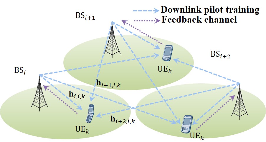
(a)

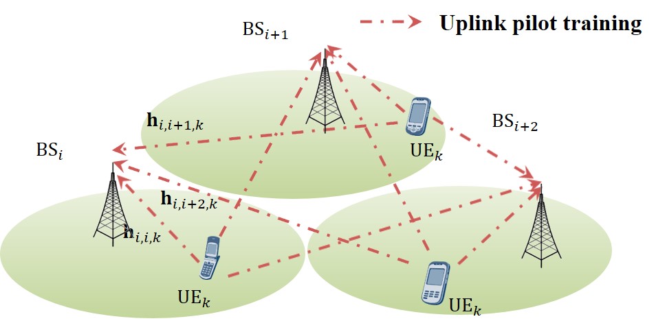
(b)

Figure 1: Pilot reuse in multiple cells. (a) FDD downlink training (b) TDD uplink training.

Several attempts have been made to tackle the challenges of acquiring high-dimensional CSI in massive MIMO. For instance, in [4], open/closed loop training that utilizes temporal and spatial channel statistics is proposed to reduce the amount of downlink training overhead. For mitigating pilot contamination, the optimal design of precoding matrices aimed at minimizing the square errors caused by pilot reuse has shown its superiority over linear precoding [5]. Thanks to the recent advances in compressed sensing [6, 7], sparse signal processing has attracted much attention in such high-dimensional settings, which has also demonstrated its power in CSI acquisition in terms of reconstructing CSI from a limited number of channel measurements. Various sparsity structures exhibited by massive MIMO channels have recently been identified, thereby motivating the development of new strategies for CSI acquisition. Surprisingly, not only can high training overhead be reduced, but pilot contamination can also be resolved by appealing to sparsity-inspired approaches.

In this paper, we provide a comprehensive overview of the state-of-the-art research on sparsity-inspired approaches for high-dimensional CSI acquisition. In Section II, the challenges in FDD and TDD massive MIMO are reviewed in detail, including a rarely mentioned issue of FDD pilot contamination. On the basis of different sparsity structures, a variety of methods for either achieving overhead reduction or alleviating the effects of pilot reuse are examined and compared in Section III. Finally, concluding remarks are made in Section IV.

Notations: $\mathbb{C}$: complex number, $\Re$: real part, $\left\|\cdot\right\|_{p}$: $p$-norm, $\left(\cdot\right){}^{{}^{\prime}}$: transpose, $\left(\cdot\right){}^{H}$: Hermitian transpose, $\mathbf{I}_{N}$: $N\times N$ identity matrix, $\mathcal{N}\left(\cdot,\cdot\right)$: normal distribution, $\mathbb{E}\left[\cdot\right]$: expectation, $\mathbf{0}$: zero vector, $\mbox{card}\left(\cdot\right)$: cardinality, $\mbox{supp}\left(\cdot\right)$: the set of indices of non-zero elements, $\mbox{Var}\left(\cdot\right)$: variance, $\max\left\{\cdot\right\}$: the maximum element, $\mbox{Vec}\left(\cdot\right)$: vectorization, $\otimes$: Kronecker product, $\succeq$: matrix inequality, $\left(\cdot\right)^{\dagger}$: pseudo inverse.

II Challenges of High-Dimensional CSI Acquisition

In massive MIMO systems with high-dimensional channels, CSI acquisition at BSs is a fundamentally challenging problem. In FDD massive MIMO, performing this task consumes a considerable amount of radio resources which is proportional to the dimension of channels. On the other hand, in TDD-mode operation, it is hard to ensure the orthogonality of pilot sequences in the multicell scenario as the number of overall UEs becomes large. As a result, the inevitable reuse of correlated pilot sequences in different cells, known as pilot contamination, causes capacity-limiting intercell interference.

To illustrate these difficulties further, we will consider a massive MIMO network consisting of $L$ hexagonal cells. In each cell, there is a BS equipped with an $M$-element linear array, serving $K$ single-antenna UEs. The channel between BS $i$ and UE $k$ in cell $j$ is denoted by the $M\times 1$ vector $\mathbf{h}_{i,j,k}$. The BS antenna size is supposed to be greatly larger than the number of served UEs.

II-A FDD Massive MIMO

In the FDD mode, obtaining CSI at BSs is normally performed in two steps. First, each BS sends a downlink training matrix to its served UEs. Second, each UE estimates the desired channel based on the downlink measurements and feeds back acquired CSI through dedicated uplink feedback channels.

During downlink training, UE $k$ in cell $i$ receives channel measurements

$$\mathbf{y}_{i,k}^{\tiny{\mbox{DL}}}=\mathbf{S}_{i}^{\tiny{\mbox{DL}}}\mathbf{h}_{i,i,k}+\sum_{l\neq i}\mathbf{S}_{l}^{\tiny{\mbox{DL}}}\mathbf{h}_{l,i,k}+\mathbf{z}_{i,k}^{\tiny{\mbox{DL}}},$$ (1)

where $\mathbf{S}_{l}^{\tiny{\mbox{DL}}}$ denotes the $N\times M$ pilot training matrix used in cell $l$, $\mathbf{z}_{i,k}^{\tiny{\mbox{DL}}}$ is the additive noise, while the first term of the right-hand side (RHS) represents the desired channel measurements, and the next term results from intercell interference. Even without considering the impact of intercell interference, the required training overhead $N$ for conventional least-squares (LS) or minimum mean square error (MMSE) estimators to achieve a reasonable performance level still scales linearly with the BS antenna size. By taking intercell interference into account, a further increase in training overhead would occur. The explicit expressions of the optimal pilot training matrices ($N\geq M$) are provided in [8] for single-cell networks. In [9], the optimal design of training matrices for multicell MIMO-OFDM systems is considered.

What makes the situation worse is that typical feedback channels are finite-rate. This implies that only quantized versions of channel estimates can be fed back to BSs. If there are predefined codebooks consisting of precoding vectors, then the index of the optimal codebook vector is required to be sent back [10, 11]. However, either the amount of quantized CSI or the size of codebooks increases in proportion to the number of BS antennas, and it in turn makes these two limited feedback techniques impractical in FDD massive MIMO.

Note that when the same training matrix is repeatedly used in multiple cells, i.e., $\mathbf{S}_{1}^{\tiny{\mbox{DL}}}=\cdots=\mathbf{S}_{L}^{\tiny{\mbox{DL}}}$, this can be regarded as pilot contamination in FDD massive MIMO. As a result of such contamination, as shown in Fig. 1(a), BS $i$ will acquire the composite channel $\sum_{l=1}^{L}\mathbf{h}_{l,i,k}$ rather than the desired channel $\mathbf{h}_{i,i,k}$, given the feedback channel being error-free and the additive noise being ignored. Despite this fact, utilizing this composite CSI to form a precoding vector and transmit signals at BS $i$ will not cause serious interference to UEs in the neighboring cells. For instance, given that maximum ratio transmission (MRT) precoding is employed, the transmitted signal from BS $i$ can be expressed as $\mathbf{x}_{i}=\sum_{k=1}^{K}\mathbf{w}_{i,k}^{\tiny{\mbox{FDD}}}x_{i,k}$ where $x_{i,k}$ is the signal intended for UE $k$ within the cell, and $\mathbf{w}_{i,k}^{\tiny{\mbox{FDD}}}=\sum_{l=1}^{L}(\mathbf{h}_{l,i,k}^{H})^{{}^{\prime}}$ denotes the MRT precoding vector. During the downlink transmission phase, the received interference at UE $m$ in cell $j$ due to BS $i$ is given by

$$I_{i,j,m} =\mathbf{h}_{i,j,m}^{{}^{\prime}}\mathbf{x}_{i}=\sum_{k=1}^{K}\sum_{l=1}^{L}\mathbf{h}_{l,i,k}^{H}\mathbf{h}_{i,j,m}x_{i,k}.$$ (2)

When the number of BS antennas grows without limit, the channel vectors are asymptotically orthogonal. Thus, the channel products $\mathbf{h}_{l,i,k}^{H}\mathbf{h}_{i,j,m}$ approach zero and so does the interference $I_{i,j,m}$. In other words, intercell interference caused by pilot contamination diminishes asymptotically with increasing BS antenna size. This implies that there is no need to mitigate intercell interference by making training matrices distinct from each other in the asymptotic regime. Hence, the existing literature rarely addresses the issue of pilot contamination in FDD massive MIMO.

Note that uplink training in the FDD mode is not considered here. An explanation for this is provided as follows. The uplink CSI is mainly utilized for data acquisition in a multiple-access channel, instead of a broadcast channel. This means that more advanced signal processing techniques, such as blind multiuser detection, can be applied at the BS side. Thus, pilot-aided training may not be the best choice and CSI acquisition is not necessarily separated from data acquisition.

II-B TDD Massive MIMO

Making massive MIMO operate in the TDD mode is a promising way to circumvent the identified difficulties in the FDD mode. Owing to channel reciprocity in the TDD mode, the CSI obtained via uplink training can be utilized for downlink transmission. More importantly, the cost of uplink training now increases linearly with the number of active UEs rather than that of BS antennas. Typically, for obtaining accurate CSI, it requires that each UE transmits an orthogonal pilot sequence to its serving BS. However, the number of available orthogonal pilot sequences is limited by the ratio of the channel coherence interval to the channel delay spread [12], which may be small due to the mobility of UEs or adverse physical environments. When the number of overall UEs becomes large, the situation of using non-orthogonal pilot sequences, known as pilot contamination, inevitably arises. A consequence of pilot contamination is intra- and inter-cell interference.

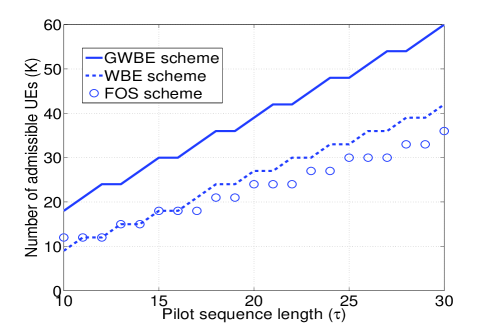
Figure 2: The number ($K=3l$) of admissible UEs versus pilot sequence length for the GWBE, WBE, and FOS schemes, given a fixed SINR-requirement pattern, that is $\left\{\gamma_{1\sim l}=\nicefrac{{1}}{{3}},\mbox{ }\gamma_{\left(l+1\right)\sim 2l}=1,\mbox{ }\gamma_{\left(2l+1\right)\sim 3l}=3\right\}$ (from [13].)

During the uplink training phase, the received signal at the $i$th BS is given by

$$\mathbf{Y}_{i}^{\tiny{\mbox{UL}}}=\sum_{l=1}^{L}\mathbf{S}_{l}^{\tiny{\mbox{UL}}}\mathbf{H}_{i,l}+\mathbf{Z}_{i}^{\tiny{\mbox{UL}}},$$ (3)

where $\mathbf{H}_{i,l}=[\mathbf{h}_{i,l,1},\ldots,\mathbf{h}_{i,l,K}]^{{}^{\prime}}$ consists of channel vectors from UEs in the $l$th cell to the $i$th BS, the columns of $\mathbf{S}_{l}^{\tiny{\mbox{UL}}}$ form a set of $\tau\times 1$ pilot sequences $\{\mathbf{s}_{l,k}\}_{k=1}^{K}$, and $\mathbf{Z}_{i}^{\tiny{\mbox{UL}}}$ denotes an additive noise matrix. To illustrate the case of intercell interference, assume that the same set of orthogonal pilot sequences is reused in each cell, i.e., $\mathbf{S}_{1}^{\tiny{\mbox{UL}}}=\cdots=\mathbf{S}_{L}^{\tiny{\mbox{UL}}}$ and $\mathbf{s}_{l,k_{1}}^{{}^{\prime}}\mathbf{s}_{l,k_{2}}=0$ for $k_{1}\neq k_{2}$, as shown in Fig. 1(b). Employing the LS estimator yields the channel estimate

$$\mathbf{\widehat{H}}_{i,i} = \left[\left(\mathbf{S}_{i}^{\tiny{\mbox{UL}}}\right)^{H}\mathbf{S}_{i}^{\tiny{\mbox{UL}}}\right]\left(\mathbf{S}_{i}^{\tiny{\mbox{UL}}}\right)^{H}\mathbf{Y}_{i}^{\tiny{\mbox{UL}}},$$ (4)

$$= \mathbf{H}_{i,i}+\sum_{l\neq i}\mathbf{H}_{i,l}+\left[\left(\mathbf{S}_{i}^{\tiny{\mbox{UL}}}\right)^{H}\mathbf{S}_{i}^{\tiny{\mbox{UL}}}\right]\left(\mathbf{S}_{i}^{\tiny{\mbox{UL}}}\right)^{H}\mathbf{Z}_{i}^{\tiny{\mbox{UL}}},$$

where the rows of $\mathbf{\widehat{H}}_{i,i}$ are given by $\mathbf{\hat{h}}_{i,i,k}=\sum_{l=1}^{L}\mathbf{h}_{i,l,k}$ when ignoring the noise. During downlink transmission, using estimates $\mathbf{\hat{h}}_{i,i,k}$ to form the transmit signal $\mathbf{x}_{i}=\sum_{k=1}^{K}\mathbf{w}_{i,k}^{\tiny{\mbox{TDD}}}x_{i,k}$, where $\mathbf{w}_{i,k}^{\tiny{\mbox{TDD}}}=\sum_{l=1}^{L}(\mathbf{h}_{i,l,k}^{H})^{{}^{\prime}}$ are MRT precoding vectors, will cause interference

$$I_{i,j,m} = \mathbf{h}_{i,j,m}^{{}^{\prime}}\mathbf{x}_{i}$$ (5)

$$= \left\|\mathbf{h}_{i,j,m}\right\|_{2}^{2}x_{i,m}+\sum_{\begin{subarray}{c}k\neq m\\ \tiny{\mbox{or }}l\neq j\end{subarray}}\mathbf{h}_{i,l,k}^{H}\mathbf{h}_{i,j,m}x_{i,k}$$

to UE $m$ in cell $j$. Though the second term on the RHS of (5) decreases with the increasing BS antenna size, the first term, which does not vanish, makes the received signal-to-interference-plus-noise ratio (SINR) at UE $m$ in cell $j$ converge to a limit and becomes the performance limiting factor.

The current investigation into TDD pilot contamination focuses on its impact on the received SINR or the sum rate when linear precoders/detectors are applied. However, very little is known about its impact on the system equipped with nonlinear precoders/detectors. A recent work [13] provides an interesting perspective on the user capacity of pilot-contaminated massive MIMO which quantifies the maximum number of admissible UEs given their own SINR requirements. As shown in Fig. 2, the user capacity of three schemes of joint pilot design and transmit power allocation is fundamentally limited by the length of pilot sequences. For further details about pilot contamination in TDD massive MIMO, the study [14] and references therein should be consulted.

III Sparsity-Inspired CSI Acquisition

Despite the challenges imposed by the high dimensionality of channel matrices, a number of research efforts have sought to address them and have achieved reasonably efficient CSI acquisition. In particular, sparsity-inspired approaches have been proved to be powerful tools, as presented below.

III-A FDD Massive MIMO

III-A1 The Joint CSI Recovery Method

Authors of [15] proposed a method for low-overhead pilot training in the single-cell scenario, taking advantage of channel sparsity. Provided that a uniform linear array with critically spaced antennas is employed at the BS, the channel $\mathbf{h}_{k}$, where indices of BSs are discarded in the single-cell scenario, exhibits a sparse representation $\mathbf{h}_{k}^{\mathrm{a}}$ in the angular domain, i.e.,

$$\mathbf{h}_{k}=\mathbf{U}\mathbf{h}_{k}^{\mathrm{a}},$$ (6)

where $\mathbf{U}$ is a discrete Fourier transform (DFT) matrix whose columns form an angular basis. The cardinality of $\mbox{supp}(\mathbf{h}_{k}^{\mathrm{a}})$ can be reasonably assumed to be greatly less than $M$ because of limited local scattering at the BS whose antenna array mounted higher than surrounding scatterers. Additionally, based on the results in [16], it has been argued that the channels to UEs are likely to share a partially common support in the angular domain, i.e., $\cap_{k=1}^{K}\mbox{supp}(\mathbf{h}_{k}^{\mathrm{a}})=\Omega_{c}$. In order to utilize the channel sparsity and common support property simultaneously, channel measurements acquired at UEs are fed back to the serving BS via error-free feedback channels. Hence, a joint channel recovery problem can be formulated as follows:

$$\begin{array}[]{cc}\underset{\left\{\mathbf{h}_{k},\forall k\right\}}{\min}&\sum_{k=1}^{K}\left\|\mathbf{y}_{k}^{\tiny{\mbox{DL}}}-\mathbf{S}^{\tiny{\mbox{DL}}}\mathbf{h}_{k}\right\|_{1}^{2}\\ \mbox{s.t.}&\cap_{k=1}^{K}\mbox{supp}(\mathbf{h}_{k}^{\mathrm{a}})=\Omega_{c}.\end{array}$$ (7)

Using orthogonal matching pursuit (OMP) as a basis, a greedy algorithm has been proposed to efficiently solve this problem. The simulation results show that the required training overhead for this recovery algorithm can be significantly less than that for the conventional LS estimator. Moreover, the mean square error (MSE) performance improves with the increasing cardinality of $\Omega_{c}$.

One major concern about this joint recovery approach is the underlying assumption of perfect channel measurements being fed back. As practical feedback channels are rate-limited, it is more reasonable to assume quantized measurements at the BS. The impact of quantization on the channel recovery performance requires further investigation. On the other hand, it has been suggested that the amount of channel measurements that is needed at the BS should be adaptively adjusted according to the sensitivity of the system performance to the CSI inaccuracy [17]. Furthermore, there has been little quantitative analysis of the required training overhead against the channel sparsity level. This quantification is in dire need as it will help us measure the actual training overhead reduction that can be achieved without relying on time-consuming simulations.

III-A2 The Weighted $\ell_{1}$ Minimization Method

Considering a similar single-cell scenario, the study in [18] has drawn attention to utilizing partial support information of sparse massive MIMO channels, which is a collection of indices of significant entries of channel vectors in the angular domain. The main advantage of using partial support information is the possibility of achieving a remarkable training overhead reduction. Specifically, the order of the required overhead decreases from $\mathcal{O}\left(s\log M\right)$ to $\mathcal{O}\left(s\right)$ where $s=\mbox{card}[\mbox{supp}(\mathbf{h}_{k}^{\mathrm{a}})]$ is the channel sparsity level. Assume that the partial support information $\widehat{T}_{k}$ of channel $\mathbf{h}_{k}^{\mathrm{a}}$ is available at UE $k$, where $\mbox{card}(\widehat{T}_{k})=\hat{s}$ and $\mbox{card}[\mbox{supp}(\mathbf{h}_{k}^{\mathrm{a}})\cap\widehat{T}_{k}]$ is given by $\left\lfloor\alpha\hat{s}\right\rfloor$. The higher the factor $\alpha$, the higher is the accuracy level of partial support information. Based on a weighted $\ell_{1}$ minimization framework, the channel recovery is performed as follows:

$$\begin{array}[]{cc}\underset{\mathbf{\hat{h}}_{k}^{\mathrm{a}}\in\mathbb{\mathbb{C}}^{M}}{\min}&\left\|\mathbf{\hat{h}}_{k}^{\mathrm{a}}\right\|_{1,\mathbf{w}}\\ \mbox{subject to}&\left\|\mathbf{S}^{\tiny{\mbox{DL}}}\mathbf{U}\mathbf{\hat{h}}_{k}^{\mathrm{a}}-\mathbf{y}_{k}^{\tiny{\mbox{DL}}}\right\|_{2}\leq\epsilon,\\ \mbox{with}&w_{i}=\begin{cases}1,&i\notin\widehat{T}_{k},\\ 0,&i\in\widehat{T}_{k},\end{cases}\mbox{ }\end{array}$$ (8)

where $\mathbf{S}^{\tiny{\mbox{DL}}}\in\mathbb{C}^{N\times M}$ is designed to be a Gaussian random matrix of independent complex normal entries, the noise $\mathbf{z}_{k}^{\tiny{\mbox{DL}}}$ is assumed to be upper bounded, i.e., $\left\|\mathbf{z}_{k}^{\tiny{\mbox{DL}}}\right\|_{2}\leq\epsilon$, and $||\mathbf{\hat{h}}_{k}^{\mathrm{a}}||_{1,\mathbf{w}}=\sum_{i=1}^{M}w_{i}|\hat{h}_{k}^{\mathrm{a}}[i]|$. In the objective function, the entries that are expected to be zero are weighted more heavily than others. The results show a significant improvement over the method without using partial support information when the accuracy level $\alpha$ exceeds a certain threshold. Moreover, taking a convex geometry approach, the authors have successfully and precisely quantified the required training overhead for achieving a certain percentage of exact recovery. The exact recovery is declared if $||\mathbf{\hat{h}}_{k}^{\mathrm{a}}-\mathbf{h}_{k}^{\mathrm{a}}||_{2}\leq 10^{-4}$. As shown in Fig. 3, the analytical curves of $\alpha=0.2$ and $\alpha=0.8$ can accurately depict the empirical phase transition curves of $60\%$ exact recovery and $55\%$ exact recovery, respectively.

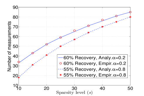
Figure 3: Phase transition curves of (8) over different values of $\alpha$ given $M=100$, $\hat{s}=10$, $\mathbf{z}_{k}^{\tiny{\mbox{DL}}}=\mathbf{0}$, and $\epsilon=0$ (from [18].)

Unlike the previous method, here, channel measurements are not fed back to the BS. In other words, it avoids the assumption of error-free feedback channels. However, it raises another issue of storing random matrices at UEs with limited memory. Also, performing convex optimization can impose a stringent computation requirement on UEs without seeking for low-complexity solutions. Several attempts have been made to design practical training matrices. In [19], Toeplitz-structured training matrices, suggested for the realistic implementation, are shown to perform comparably to Gaussian random matrices and require generating less independent random variables. A deterministic approach to the training matrix design is first considered by appealing to matrix properties such as mutual coherence [20]. More advanced deterministic training matrices are developed in [21] to yield higher recovery accuracy. In the context of FDD massive MIMO, it would be interesting to invent structurally random or deterministic training matrices that take partial support information of channels to multiple UEs into consideration. In addition, the similar concepts of using prior channel knowledge to lower training overhead can be found in [4] where spatial and temporal correlations are harnessed. More study is needed to better understand how to integrate all the relevant prior knowledge into efficient CSI acquisition.

III-B TDD Massive MIMO

As mentioned in Sec. II-B, employing uplink training to obtain high-dimensional downlink CSI results in undesired pilot contamination, and the following are some efforts to address this issue.

III-B1 The Coordinated MMSE Method

Contradicting conventional wisdom, it has been shown that it is possible to mitigate pilot contamination using the linear MMSE estimator [22]. The key factor in determining the success of MMSE estimation is that each channel to the UE can be regarded as a linear combination of finite steering vectors

$$\mathbf{h}_{i,j,k}=\frac{1}{\sqrt{P}}\sum_{p=1}^{P}\alpha_{i,j,k}\left(p\right)\mathbf{a}\left[\theta_{i,j,k}\left(p\right)\right],$$ (9)

where $P$ is the number of paths, $\alpha_{i,j,k}\left(p\right)$ are zero-mean path gains, and $\mathbf{a}\left[\theta_{i,j,k}\left(p\right)\right]$ denote the steering vectors due to angle of arrivals (AoAs) $\theta_{i,j,k}\left(p\right)$. Consequently, the rank of the channel covariance matrix $\mathbf{R}_{i,j,k}\triangleq\mathbb{E}\{\mathbf{h}_{i,j,k}\mathbf{h}_{i,j,k}^{H}\}$ depends on the range $[\theta_{i,j,k}^{\min},\theta_{i,j,k}^{\max}]$ in which AoAs $\theta_{i,j,k}\left(p\right)$ lie, which typically turns out to be low. Let us focus on the $k$th row of (4), i.e., $\mathbf{\hat{h}}_{i,i,k}=\sum_{l=1}^{L}\mathbf{h}_{i,l,k}+\mathbf{z}_{i,k}$. Based on it, the desired channel $\mathbf{h}_{i,i,k}$ can be further extracted by the MMSE estimator, i.e.,

$$\mathbf{\hat{\hat{h}}}_{i,i,k} = \mathbf{R}_{i,i,k}\left(\sigma_{z}^{2}\mathbf{I}_{M}+\sum_{l=1}^{L}\mathbf{R}_{i,l,k}\right)^{-1}\mathbf{\hat{h}}_{i,i,k},$$ (10)

where the covariance matrix of $\mathbf{z}_{i,k}$ is assumed to be $\sigma_{z}^{2}\mathbf{I}_{M}$. When the range of AoAs due to interfering UEs that use the same pilot sequence does not overlap with the AoA range due to the desired UE, the estimate $\mathbf{\hat{\hat{h}}}_{i,i,k}$ approaches the desired $\mathbf{h}_{i,i,k}$ as the BS antenna size grows to infinity. This feature is highly attractive because the dimension of the BS antennas can be made as large as desired in massive MIMO. Moreover, the condition of non-overlapping AoA ranges can be satisfied if the reused pilot sequence is properly allocated to UEs in neighboring cells. A heuristic algorithm has been developed to perform pilot allocation in a coordinated manner. Another favorable feature of this method recently demonstrated in [23] is that the asymptotically optimal estimate is obtainable whether uniform or non-uniform arrays are employed. As a result, BS antenna arrays are exempt from the requirement of high calibration accuracy.

The second-order statistics of high-dimensional channels have successfully been utilized to facilitate robust MMSE channel estimation under pilot contamination. However, obtaining channel covariance matrices of high dimension imposes another challenge to the massive MIMO system. It is interesting to know if the low-rankness can help speed up the acquisition of channel covariance matrices. Furthermore, it is still unknown if this covariance-matrix-aware method is sensitive to the inaccuracy of the second-order statistics. On the other hand, the information about AoAs actually can be extracted from statistical channel knowledge prior to commencing the instantaneous CSI acquisition [24]. In this case, the dimension of the parameter space of each channel shrinks to $P$, which can be significantly less than the original. Most importantly, this information could aid BSs in distinguishing between training signals from UEs using the same pilot.

TABLE I: Comparison of Sparsity-Inspired CSI Acquisition Methods

Methods	Sparsity Types	Pros	Cons
Joint CSI Recovery (FDD)	Sparse channel vectors & Common supports	• Jointly exploit sparsity & common-support property • Perform channel recovery at the BS	• UEs need to feed back perfect channel measurements
Weighted $\ell_{1}$Minimization (FDD)	Sparse channel vectors & partial support information	• Sharp estimate of the required training overhead • Lower training overhead	• Need to obtain partial support information
Coordinated MMSE (TDD)	Low-rank channel covariance matrices	• Performance improves with increasing antenna size • Lower training overhead	• Need to obtain second-order channel statistics
Quadratic SDP (TDD)	Low-rank channel matrices	• No need for knowledge of second-order channel statistics	• Only suitable for poor scattering propagation environments • Higher training overhead
Sparse Bayesian Learning (TDD)	Sparse channel vectors in the UE domain	• No need for knowledge of second-order channel statistics	• Channels are not jointly recovered • Higher training overhead

III-B2 The Quadratic Semidefinite Programming (SDP) Method

It is suggested that a BS should collect CSI of both the desired links within the cell and interference links from its neighboring cells [25]. In other words, the CSI of interference links should not be regarded as irrelevant information. From this new angle, the expression (3) can be recast as

$$\mathbf{Y}_{i}^{\tiny{\mbox{UL}}}=\mathbf{\underline{S}}^{\tiny{\mbox{UL}}}\mathbf{H}_{i}+\mathbf{Z}_{i}^{\tiny{\mbox{UL}}},$$ (11)

where $\mathbf{\underline{S}}^{\tiny{\mbox{UL}}}\triangleq[\mathbf{S}_{1}^{\tiny{\mbox{UL}}},\ldots,\mathbf{S}_{L}^{\tiny{\mbox{UL}}}]$ and $\mathbf{H}_{i}\triangleq[\mathbf{H}_{i,1}^{{}^{\prime}},\ldots,\mathbf{H}_{i,L}^{{}^{\prime}}]^{{}^{\prime}}$ is the full CSI of wireless links that should be recovered. Thus, the currently challenging issue is similar to that in FDD massive MIMO, i.e., how to reduce the required training overhead.

In the undesirable scattering propagation environments, the rank of the channel matrix is equal to the number $r$ of the feasible AoAs $\theta_{i,j,k}\left(p\right)$ in (9), which is greatly less than $\max\left\{M,K\cdot L\right\}$. Based on this observation, a unclear norm regularized problem can be formulated as

$$\begin{array}[]{cc}\underset{\mathbf{H}_{i}}{\min}&\frac{1}{2}\left\|\mbox{vec}\left(\mathbf{Y}_{i}^{\tiny{\mbox{UL}}}\right)-\Psi\mbox{vec}\left(\mathbf{H}_{i}\right)\right\|_{2}^{2}+\gamma\left\|\mathbf{H}_{i}\right\|_{F}\end{array},$$ (12)

where $\Psi=\mathbf{\underline{S}}^{\tiny{\mbox{UL}}}\otimes\mathbf{I}_{M}$ and $\gamma$ is a regularization factor. The sole purpose of adopting unclear norm regulation is to minimize the sum of the matrix’s singular values, thereby achieving rank minimization. The above problem has been further recast as a quadratic SDP problem

$$\begin{array}[]{cc}\underset{\mathbf{v}}{\min}&\frac{1}{2}\mathbf{v}^{H}\mathbf{v}-\Re\left\{\left[\mbox{vec}\left(\mathbf{Y}_{i}^{\tiny{\mbox{UL}}}\right)\right]^{H}\mathbf{v}\right\}\\ \mbox{s.t.}&\left[\begin{array}[]{cc}\gamma\mathbf{I}_{KL}&\mbox{vec}_{KL,M}^{-1}\left(\Psi^{H}\mathbf{v}\right)\\ \left[\mbox{vec}_{KL,M}^{-1}\left(\Psi^{H}\mathbf{v}\right)\right]^{H}&\gamma\mathbf{I}_{M}\end{array}\right]\succeq 0.\end{array}$$ (13)

The solution $\mathbf{v}^{*}$ to this SDP problem determines the estimate of the channel matrix

$$\mathbf{H}_{i}^{*}=\mbox{vec}_{KL,M}^{-1}\left\{\Psi^{\dagger}\left[\mbox{vec}\left(\mathbf{Y}_{i}^{\tiny{\mbox{UL}}}\right)-\mathbf{v}^{*}\right]\right\},$$ (14)

which can now be obtained efficiently, thanks to the readily available polynomial-time SDP solvers.

In the commencing study of massive MIMO [26], the CSI of interference links at BSs is viewed as nonessential. This is because that desired links and interference links are asymptotically orthogonal, and more importantly, intercell interference can be proved manageable with the CSI of desired links only. Here, we offer an explanation why there is a need for acquiring the CSI of interference links in the poor scattering environments. Consider that $\mathbf{H}_{i}=\mathbf{G}_{i}\mathbf{A}$ where $\mathbf{A}=[\mathbf{a}\left(\phi_{1}\right),\ldots,\mathbf{a}\left(\phi_{r}\right)]^{{}^{\prime}}$ is an $r\times M$ matrix of full row rank with $r\ll\min\left\{M,KL\right\}$ due to poor scattering, and $\mathbf{G}_{i}$ consists of $KL\times r$ independent and identically distributed (i.i.d.) zero-mean channel gains. Then, we have $\lim_{M\rightarrow\infty}\mathbf{A}\mathbf{A}^{H}=\mathbf{I}_{r}$ and

$$\lim_{M\rightarrow\infty}\mathbf{H}_{i}\mathbf{H}_{i}^{H}=\mathbf{G}_{i}\mathbf{G}_{i}^{H}\not\propto\mathbf{I}_{KL}$$ (15)

which implies that the correlation among wireless links does not diminish with the increasing BS antenna size. In such a situation, it becomes crucial to obtain the full CSI of wireless links for effective interference management.

III-B3 The Sparse Bayesian Learning (SBL) Method

Sharing the same perspective as the study [25], the work in [27] also considers acquiring the full CSI of wireless links and proposes a sparse Bayesian learning method to achieve this goal. Sparse Bayesian learning was first presented in [28] and has been proved to outperform some prevailing $\ell_{1}$ minimization algorithms [29]. The SBL method proceeds by first transforming the channel matrix into the angular domain via DFT as mentioned in the joint CSI recovery method, i.e., $\mathbf{\underline{H}}_{i}=\mathbf{H}_{i}\mathbf{U}$. Interestingly, instead of taking advantage of the sparsity in the angular domain, the sparsity in the UE domain, which has been empirically shown to exist, is utilized. In other words, the column vectors of the channel matrix $\mathbf{\underline{H}}_{i}$ are considered one by one. As each column vector consists of elements due to different UEs, the independence among elements can be reasonably assumed. This independence together with the sparsity in the UE domain leads to an effective Gaussian-mixture (GM) model which well describes the joint distributions of the channel elements. More surprisingly, empirical results show that there are only few parameters involved in the GM model that need to be determined. Therefore, the practical Bayes estimation can be implemented by evaluating marginal probability density functions via the approximate message passing (AMP) algorithm [30] and learning GM parameters by means of the expectation-maximization (EM) algorithm [31]. The numerical results show that this Bayesian method can achieve a significant reduction in estimation errors.

The assumption of channel vectors being sparse in the UE domain may not hold when the UE dimension $KL$ is not large enough. A possible remedy for this situation is suggested in the following. First, it is desirable to understand if the GM model is also applicable for modeling distributions of spare channel vectors in the angular domain. Second, as angular-domain channels are very likely to consist of a small number of block-wise non-zero segments resulting from few clusters of scatterers, it is eminently reasonable to assume some dependence among angular-domain channel elements. Hence, the distribution of the channel vector could be a mixture of Gaussian random vectors, and the original AMP and EM algorithms should be modified accordingly to this new GM model.

III-C Discussion and Comparison

In the previous subsections, several methods for efficient high-dimensional CSI acquisition have been discussed for massive MIMO communications. Table I provides a brief summary of the advantages and disadvantages of these methods. It is shown in the table that each method utilizes a distinct sparsity structure. However, all sparsity structures considered in massive MIMO are based on the observation that angular-domain channels are sparse. As a result, the second-order statistics of massive MIMO channels inherit the sparsity structure, yielding low-rank channel covariance matrices. In addition, as sparse channels are collectively examined, it leads to either block-sparse or low-rank channel matrices. When the UE dimension is comparable to the channel dimension, sparsity in the angular domain also results in sparsity in the UE domain. On the basis of the aforementioned sparsity structures, different sparsity-inspired methods are developed either to reduce training overhead or to mitigate pilot contamination.

In FDD massive MIMO, without feeding back channel measurements to the BS side, less sparsity structures are available for developing efficient CSI acquisition methods. Despite this limitation, the weighted $\ell_{1}$ minimization method shows that achieving further overhead reduction is feasible if partial support information can be obtained in advance and properly harnessed. Interestingly, by enabling the BS to gather perfect channel measurements from its served UEs, the joint CSI recovery method offers an effective way of utilizing sparsity structures across multiple UEs. If the performance superiority of this method still holds when taking rate-limited feedback channels into account, it will establish the fact that offloading CSI acquisition tasks to the BS is feasible and beneficial.

With regard to TDD massive MIMO, uplink training has more sparsity structures to utilize as high-dimensional channels are jointly recovered at the BS side. It is worth noting that only low-rank channel covariance matrices have been used for pilot decontamination. Other sparsity structures such as low-rank channel matrices and sparse UE-domain channels have not been considered for mitigating the effects of pilot reuse. In this regard, there is still much room for innovation in sparsity-inspired pilot decontamination. It is also worth noting that using perfect covariance matrices of both desired channels and interference channels in the coordinated MMSE method has drawn criticism [32]. It would be intriguing to assess if there exist efficient algorithms for learning low-rank covariance matrices. If such algorithms are developed or identified, they should be integrated into the coordinated MMSE method.

III-D Implementation Issues

Recently investigators have examined the practical implementation of compressed sensing based algorithms for sparse channel recovery [33, 34, 35]. Although the design targets are channel models in the 3GPP LTE standard, several insights that have been provided are still valuable and applicable to realistic implementation of sparse massive MIMO channel recovery. It has been pointed out that greedy algorithms such as OMP or matching pursuit (MP) are more desirable from a hardware perspective. It is because these algorithms require lower computational complexity and lower numerical precision when compared to convex relaxation algorithms such as basis pursuit (BP) [34]. The trade-off between hardware complexity and denoising performance of three greedy algorithms has been characterized in [35] and it is indicated that the chip area overhead required to implement the gradient pursuit (GP) algorithm can be three times larger than MP. The power consumption is normally proportional to this area overhead. When it comes to the design of channel recovery algorithms in FDD massive MIMO, which are typically performed at the UE side, the issue of hardware complexity should be carefully taken into account. On the other hand, at the BS side, high-dimensional channels can be recovered by more advanced algorithms such as sparse Bayesian learning or joint CSI recovery.

III-E Implications of New Propagation Models

Most existing studies have based their CSI acquisition approaches on the conventional MIMO channel models, which may fail to capture some unique characteristics of massive MIMO channels. For instance, the far-field and plane wavefront assumptions no longer hold when antenna arrays become physically larger than the Rayleigh distance [36]. On the other hand, the sheer size of antenna arrays, where different antenna elements observe varying subsets of scatterer clusters, makes the assumption of spatial channels being wide-sense stationary on the array axis no longer valid [37]. While new channel models have been proposed in [38, 39] by making a more accurate spherical wavefront assumption and taking the non-stationarities into consideration, there is still very little understanding of how these characteristics affect the sparsity structures of the channels in massive MIMO systems. One previous result [40], however, suggests that the spherical wavefront model does adequately characterize the rank of the channel matrix. This implies that the new channel models can potentially affect the SDP method which exploits the sparsity in the form of the channel matrix rank. In addition, the possibility that none of clusters are perceptible to some antenna elements cannot be categorically excluded, so it indicates the possible presence of the sparsity on the array axis. These inferences suggest that there is abundant room for further progress in identifying utilizable sparsity structures based on the latest models.

IV Conclusions

In this article, the challenges of acquiring high-dimensional CSI in FDD/TDD massive MIMO systems have been discussed. To address these challenges and break the curse of dimensionality, one can effectively utilize sparsity structures that uniquely appear in massive MIMO channels. Several state-of-the-art sparsity-inspired approaches for high-dimensional CSI acquisition have been examined and compared in terms of the sparsity structures being exploited, while their own advantages and disadvantages are identified. As a result of this study, the following conclusions can be drawn. The sparsity structures that can be harnessed are conditional on the radio propagation environments. In TDD massive MIMO, uplink training inherently has more sparsity structures to exploit as high-dimensional channels are jointly recovered at the BS. On the contrary, in the FDD mode, the desired channel is normally recovered at the UE where utilizable sparsity structures are limited. Finally, based upon existing approaches, we have identified the potential research problems in need of further investigation.

References

- [1] T. Marzetta, “Noncooperative cellular wireless with unlimited numbers of base station antennas,” IEEE Trans. Wireless Commun., vol. 9, no. 11, pp. 3590–3600, Nov. 2010.
- [2] F. Rusek, D. Persson, B. K. Lau, E. Larsson, T. Marzetta, O. Edfors, and F. Tufvesson, “Scaling up MIMO: Opportunities and challenges with very large arrays,” IEEE Signal Process. Mag., vol. 30, no. 1, pp. 40–60, 2013.
- [3] G. Bartoli, R. Fantacci, K. B. Letaief, D. Marabissi, N. Privitera, M. Pucci, and J. Zhang, “Beamforming for small cell deployment in LTE-advanced and beyond,” IEEE Wireless Commun., vol. 21, no. 2, pp. 50–56, Apr. 2014.
- [4] J. Choi, D. Love, and P. Bidigare, “Downlink training techniques for FDD massive MIMO systems: Open-loop and closed-loop training with memory,” IEEE J. Sel. Topics Signal Process., vol. 8, no. 5, pp. 802–814, Oct. 2014.
- [5] J. Jose, A. Ashikhmin, T. Marzetta, and S. Vishwanath, “Pilot contamination and precoding in multi-cell TDD systems,” IEEE Trans. Wireless Commun., vol. 10, no. 8, pp. 2640–2651, Aug. 2011.
- [6] W. Bajwa, J. Haupt, A. Sayeed, and R. Nowak, “Compressed channel sensing: A new approach to estimating sparse multipath channels,” Proc. IEEE, vol. 98, no. 6, pp. 1058–1076, Jun. 2010.
- [7] Y. C. Eldar and G. Kutyniok, Compressed Sensing: Theory and Applications. Cambridge University Press, 2012.
- [8] M. Biguesh and A. Gershman, “Training-based MIMO channel estimation: A study of estimator tradeoffs and optimal training signals,” IEEE Trans. Signal Process., vol. 54, no. 3, pp. 884–893, Mar. 2006.
- [9] J. W. Kang, Y. Whang, H. Y. Lee, and K. S. Kim, “Optimal pilot sequence design for multi-cell MIMO-OFDM systems,” IEEE Trans. Wireless Commun., vol. 10, no. 10, pp. 3354–3367, Oct. 2011.
- [10] D. Love, R. Heath, V. Lau, D. Gesbert, B. Rao, and M. Andrews, “An overview of limited feedback in wireless communication systems,” IEEE J. Sel. Areas Commun., vol. 26, no. 8, pp. 1341–1365, Oct. 2008.
- [11] A. Ghosh, J. Zhang, J. G. Andrews, and R. Muhamed, Fundamentals of LTE. Prentice-Hall, 2010.
- [12] E. Larsson, O. Edfors, F. Tufvesson, and T. Marzetta, “Massive MIMO for next generation wireless systems,” IEEE Communications Magazine, vol. 52, no. 2, pp. 186–195, Feb. 2014.
- [13] J.-C. Shen, J. Zhang, and K. B. Letaief, “User capacity of pilot-contaminated TDD massive MIMO systems,” in Proc. IEEE Global Commun. Conf. (Globecom), Austin, TX, Dec. 2014.
- [14] L. Lu, G. Li, A. Swindlehurst, A. Ashikhmin, and R. Zhang, “An overview of massive MIMO: Benefits and challenges,” IEEE J. Sel. Topics Signal Process., vol. 8, no. 5, pp. 742–758, Oct. 2014.
- [15] X. Rao and V. Lau, “Distributed compressive CSIT estimation and feedback for FDD multi-user massive MIMO systems,” IEEE Trans. Signal Process., vol. 62, no. 12, pp. 3261–3271, Jun. 2014.
- [16] J. Poutanen, K. Haneda, J. Salmi, V. Kolmonen, F. Tufvesson, T. Hult, and P. Vainikainen, “Significance of common scatterers in multi-link indoor radio wave propagation,” in Proc. 4th Eur. Conf. Antennas Propag. (EuCAP), Barcelona, Spain, Apr. 2010, pp. 1–5.
- [17] P.-H. Kuo, H. Kung, and P.-A. Ting, “Compressive sensing based channel feedback protocols for spatially-correlated massive antenna arrays,” in Proc. IEEE Wireless Commun. Netw. Conf. (WCNC), Shanghai, China, Apr. 2012, pp. 492–497.
- [18] J.-C. Shen, J. Zhang, E. Alsusa, and K. B. Letaief, “Compressed CSI acquisition in FDD massive MIMO with partial support information,” to be presented at the IEEE Int. Conf. Commun. (ICC), London, UK, 2015.
- [19] W. Bajwa, J. Haupt, G. M. Raz, S. Wright, and R. Nowak, “Toeplitz-structured compressed sensing matrices,” in Proc. IEEE/SP 14th Workshop Statist. Signal Process., Madison, WI, Aug. 2007, pp. 294–298.
- [20] M. Elad, “Optimized projections for compressed sensing,” IEEE Trans. Signal Process., vol. 55, no. 12, pp. 5695–5702, Dec. 2007.
- [21] G. Li, Z. Zhu, D. Yang, L. Chang, and H. Bai, “On projection matrix optimization for compressive sensing systems,” IEEE Trans. Signal Process., vol. 61, no. 11, pp. 2887–2898, Jun. 2013.
- [22] H. Yin, D. Gesbert, M. Filippou, and Y. Liu, “A coordinated approach to channel estimation in large-scale multiple-antenna systems,” IEEE J. Sel. Areas Commun., vol. 31, no. 2, pp. 264–273, Feb. 2013.
- [23] H. Yin, D. Gesbert, and L. Cottatellucci, “Dealing with Interference in distributed large-scale MIMO systems: A statistical approach,” IEEE J. Sel. Topics Signal Process., vol. 8, no. 5, pp. 942–953, Oct. 2014.
- [24] J. Foutz, A. Spanias, and M. K. Banavar, Narrowband Direction of Arrival Estimation for Antenna Arrays. Morgan & Claypool Publishers, 2008.
- [25] S. L. H. Nguyen and A. Ghrayeb, “Compressive sensing-based channel estimation for massive multiuser MIMO systems,” in Proc. IEEE Wireless Commun. Netw. Conf. (WCNC), Shanghai, China, Apr. 2013, pp. 2890–2895.
- [26] T. Marzetta, “How much training is required for multiuser MIMO,” in Proc. 40th Asilomar Conf. Signals, Syst., Comput. (ACSSC), Pacific Grove, CA, Oct. 2006, pp. 359–363.
- [27] C.-K. Wen, S. Jin, K.-K. Wong, J.-C. Chen, and P. Ting, “Channel estimation for massive MIMO using Gaussian-mixture Bayesian learning,” IEEE Trans. Wireless Commun., 2014.
- [28] M. E. Tipping, “Sparse Bayesian learning and the relevance vector machine,” J. Mach. Learn. Res., vol. 1, pp. 211–244, Sept. 2001.
- [29] Z. Zhang and B. Rao, “Sparse signal recovery with temporally correlated source vectors using sparse Bayesian learning,” IEEE J. Sel. Topics Signal Process., vol. 5, no. 5, pp. 912–926, Sept. 2011.
- [30] D. L. Donoho, A. Maleki, and A. Montanari, “Message-passing algorithms for compressed sensing,” Proc. Nat. Acad. Sci., vol. 106, no. 45, pp. 18 914–18 919, Nov. 2009.
- [31] J. Vila and P. Schniter, “Expectation-maximization Gaussian-mixture approximate message passing,” IEEE Trans. Signal Process., vol. 61, no. 19, pp. 4658–4672, Oct. 2013.
- [32] J. Zhang, B. Zhang, S. Chen, X. Mu, M. El-Hajjar, and L. Hanzo, “Pilot contamination elimination for large-scale multiple-antenna aided OFDM systems,” IEEE J. Sel. Topics Signal Process., vol. 8, no. 5, pp. 759–772, Oct. 2014.
- [33] J. Lofgren, L. Liu, O. Edfors, and P. Nilsson, “Improved matching-pursuit implementation for LTE channel estimation,” IEEE Trans. Circuits Syst. I: Reg. Papers, vol. 61, no. 1, pp. 226–237, Jan. 2014.
- [34] P. Maechler, P. Greisen, N. Felber, and A. Burg, “Matching pursuit: Evaluation and implementatio for LTE channel estimation,” in Proc. IEEE Int. Symp. Circuits Syst. (ISCAS), Paris, France, May 2010, pp. 589–592.
- [35] P. Maechler, P. Greisen, B. Sporrer, S. Steiner, N. Felber, and A. Burg, “Implementation of greedy algorithms for LTE sparse channel estimation,” in Proc. Asilomar Conf. Signals, Syst., Comp. (ASILOMAR), Pacific Grove, CA, Nov. 2010, pp. 400–405.
- [36] S. Payami and F. Tufvesson, “Channel measurements and analysis for very large array systems at 2.6 GHz,” in Proc. Europ. Conf. Antennas Propag. (EUCAP), Prague, Czech Republic, Mar. 2012, pp. 433–437.
- [37] X. Gao, F. Tufvesson, and O. Edfors, “Massive mimo channels - measurements and models,” in Proc. 47th Annu. Asilomar Conf. Signals, Syst., Comput., Pacific Grove, CA, Nov. 2013, pp. 280–284.
- [38] S. Wu, C.-X. Wang, E.-H. Aggoune, M. Alwakeel, and Y. He, “A non-stationary 3-D wideband twin-cluster model for 5G massive MIMO channels,” IEEE J. Sel. Areas Commun., vol. 32, no. 6, pp. 1207–1218, Jun. 2014.
- [39] S. Wu, C.-X. Wang, H. Haas, E.-H. Aggoune, M. Alwakeel, and B. Ai, “A non-stationary wideband channel model for massive MIMO communication systems,” IEEE Trans. Wireless Commun., vol. 14, no. 3, pp. 1434–1446, Mar. 2015.
- [40] J.-S. Jiang and M. Ingram, “Spherical-wave model for short-range MIMO,” IEEE Trans. Commun., vol. 53, no. 9, pp. 1534–1541, Sept. 2005.