Optimal Time-Series Motifs

Abstract

Motifs are the most repetitive/frequent patterns of a time-series. The discovery of motifs is crucial for practitioners in order to understand and interpret the phenomena occurring in sequential data. Currently, motifs are searched among series sub-sequences, aiming at selecting the most frequently occurring ones. Search-based methods, which try out series sub-sequence as motif candidates, are currently believed to be the best methods in finding the most frequent patterns.

However, this paper proposes an entirely new perspective in finding motifs. We demonstrate that searching is non-optimal since the domain of motifs is restricted, and instead we propose a principled optimization approach able to find optimal motifs. We treat the occurrence frequency as a function and time-series motifs as its parameters, therefore we learn the optimal motifs that maximize the frequency function. In contrast to searching, our method is able to discover the most repetitive patterns (hence optimal), even in cases where they do not explicitly occur as sub-sequences. Experiments on several real-life time-series datasets show that the motifs found by our method are highly more frequent than the ones found through searching, for exactly the same distance threshold.

1 Introduction

Time-series are arguably the most widespread type of data which occur in virtually all the application domains of our modern lives, wherever measurements have associated time stamps (e.g.: physiological and medical, financial, meteorological, sound and video, monitoring system sensors, astronomy light intensities, and many more ).

In many cases, the underlying patterns of those datasets are not known to the domain practitioners and a visual inspection is often infeasible given the complexity and size of the data. For this reason, finding the most repetitive patterns in time-series help the domain experts understand the underlying phenomena within diverse sources of data  [2, 26]. The most repetitive time-series patterns are called motifs and their discovery has recently attracted considerable research [25, 20, 30, 14]. In brief terms, optimal motifs are those which repeat the most (i.e. have the highest frequency) given a distance/similarity threshold value. The approach of the current state-of-the-art motif discovery methods is to search the motifs from the segments (a.k.a sub-sequences) of time series [25, 28, 14, 3]. More concretely, series segments are considered to be motif candidates and the most frequent segments are sorted out.

In this paper we present an entirely new and orthogonally different perspective to the search-based approach. First of all, we treat frequency as a function and motifs as its variable. Naturally our task becomes finding the values of motifs which maximize the value of the frequency function. In this perspective we formalize motif discovery as a principled optimization problem and devise an optimization technique to learn the optimal motifs. The learning process uses the first order derivative of the frequency function, in order to find its maximum. In that way, our method can learn motifs which yield the maximum frequency (a.k.a the highest number of matches). The proposed learning method is theoretically superior to the search-based approach, because in the case of searching the motif candidates are limited to the domain of sub-sequences and cannot discover latent series patterns (Section 4.1) .

As the empirical results (Section 6) over various real-life datasets will indicate, our optimal motifs have significantly more matches (higher frequency) than the ones found through searching, for exactly the same distance threshold.

2 Related Work

The research on discovering time-series motifs has suffered from a terminological ambiguity. Initially, motifs were defined to be the most frequently occurring patterns in a time-series [25]. However, another stream of papers redefined the term "motif" as the closest pair among series segments [23, 21]. In this paper we mean "the most frequently occurring patterns" [25] when referring to motifs. The closest pair of series segments, on the other hand, will be referred to as "pair-motif" following the suggestion of [19].

2.1 Pair-motif discovery

The closest pair of series segments can be perceived as a sub-variation of the general motif discovery task. The brute-force search that computes the distance of every segment pair is computationally expensive, therefore efforts are devoted towards scaling the brute force up. A fast, yet exact, method that discovers pair-wise motifs has been introduced by [23]. Enumerations of all motifs having variable lengths has also been researched [20, 19]. In a streaming scenario an algorithm can not rely on accessing the full past series, therefore we need to find the top-k motif search via an on-line method as in [12]. In addition, the statistical significance of the motifs found has also been a topic of interest [4, 5].

Note: Finding motif-pairs is equivalent to the problem of locating the closest pair of points in a geometrical space and is a historic problem in computational geometry [8].

2.2 Motif Discovery

Repeating patterns in sequential data have initially been studied in bio-informatics [2]. However, finding motifs is beneficial in understanding physiological human data [26], while being also useful in understanding behavioral patterns of living organisms [1]. The concept of recurrent patterns was transferred to the realm of time-series data under the term "motifs" [25] and a search-based approach to discovering motifs was proposed. In order to find motifs that are immune to noisy variations, a probabilistic search of time-series motifs was based on random projections [7]. Another work has explored the employment of uniform scaling as the similarity distance used for discovering the motifs [28]. Furthermore, a hybrid combination of supervised and unsupervised learning has been used for searching recurring patterns [24]. The first step involves a teacher which labels whether or not a time series includes a particular pattern, while in the next step an unsupervised learning from the series in order to reconstruct the teacher is exploited. The task of finding the most recurring motifs has also been tackled through searching for candidate motifs organized in a tree structure [15].

The brute-force approach which tries out every segment (sub-sequence) as a potential motif has a quadratic complexity in the number of segments. Therefore approximate motif discovery methods have been exploited. Conversion of motifs into a symbolic representation (named SAX) is a pre-processing alternative [10]. Over the new representation an agglomerative clustering can be used to find motifs [10]. A scalable alternative that can approximately discover multi-resolution motifs in a single scan utilizes different cardinalities of the symbolic representation [3]. Last but not least, a scalable version of the pair-wise motifs has been extended to the general motifs discovery for large-scale data [22].

Given the widespread of multi-dimensional time series, there has also been interest in mining multi-dimensional motifs too. Several strategies were inspected, where motifs span all versus a subset of the dimensions, with or without temporal overlap [17]. The algorithm is based on random projections of the symbolic sub-sequence representations [17]. Discovering regions of high density in the space of sub-sequencies is another alternative to mining multivariate motifs [18]. Graph clustering implemented as a two-staged algorithm was also employed in detecting multidimensional motifs [27]. In the first step single-dimensional motifs are discovered and later blended through clustering [27].

Since motifs are previously unknown patterns, there is little information on the motifs’ lengths too. Under such a reality authors attempted to discover the optimal motif length, for instance by inspecting the compressibility of the data [30]. In addition, variable-length motifs can be extracted using a grammar-inspired inference process [13]. Interest has been attracted in terms of visualizing variable-length motifs [14], finding them in linear time [6], or using them for classification purposes [29].

In contrast to the related work, our novel contribution relies in computing an optimal set of motifs given a threshold distance and the motifs’ length. We are the first to propose a principled optimization method for the task. As a consequence, our approach leads to significantly improved motif quality (frequency) compared to brute-force search.

3 Preliminaries

3.1 Notations

3.1.1 Time Series and Motifs

A time series is a long ordered sequence of real-valued measurements. Such a series is abstracted as a list of $J$-many Z-normalized sliding-window segments of length $L$ and is denoted as $S\in{\mathbb{R}}^{J\times L}$. On the other hand, a repetitive pattern, a.k.a motif, is simply a sequence of $L$ points. The definition can be generalized to a set of $K$-motifs and consecutively denoted as $M\in{\mathbb{R}}^{K\times L}$.

3.1.2 Motif Frequency

The occurrence frequency of a motif is defined as the nontrivial (see Section 3.2.2) number of matches between a motif and all the normalized segments of the time series. The current approach of counting the matching frequency of the $k$-th motif, denoted $M_{k,:}\in{\mathbb{R}}^{L}$, iterates over all the $j\in\{1,\dots,J\}$ sliding window segments $S_{j,:}$ and check whether the motif of interest matches the segments within a threshold distance $T\in{\mathbb{R}}^{+}$.

$$\mathcal{F}(M) = \sum_{k=1}^{K}\sum_{j=1}^{J}\mathcal{F}_{k,j}$$ (1)

$$\mathcal{F}_{k,j} = \begin{cases}1&\text{if }\left(\sum_{l=1}^{L}\left(M_{k,l}-S_{j,l}\right)^{2}\right)<T\\ 0&\text{otherwise}\end{cases}$$ (2)

Equation 1 presents the formalism for the overall frequency as a sum of motifs’ frequencies, while Equation 2 encapsulates the concept of a match. If the distance between a segment $S_{j,:}$ and a motif $M_{k,:}$ is less than the threshold $T$, then a matching value of one is granted.

3.2 Problem Definition

3.2.1 Optimal Motifs

Following the established literature definition, the only optimality criterion of a motif is its frequency at a particular distance threshold. Therefore, the only legitimate metric to compare the qualities of motifs is frequency (a.k.a. support, or number of matches). The optimal motifs $M^{*}$ for a time series are defined in Equation 3.2.1 as the candidate motifs $M$ that achieve the maximum frequency value $\mathcal{F}(M)$ from Equation 1. There is, nevertheless, an important constraint in the search for motifs: The $K$ motifs should be different from each other [25], otherwise, the motifs risk being close variations of the single most repetitive motif. Such a constraint is presented under a "such that (s.t.)" clause in Equation 3.2.1, which enforces each pair of motifs $(M_{k,:},M_{p,:})$ to be different from each other by a distance of at least $2T$ (so each pair does not overlap within a threshold $T$, details in [25]).

$$M^{*} := \operatorname*{\operatorname{argmax}}_{M\in{\mathbb{R}}^{K\times L}}\;\;\;\mathcal{F}(M)$$

s.t.: $$\left(\sum_{l=1}^{L}\left(M_{k,l}-M_{p,l}\right)^{2}\right)>2T,$$

$$\forall k\in\{1,\dots,K\},\forall p\in\{k+1,\dots,K\}$$

3.2.2 Trivial Matches

Stated shortly, trivial matches are consecutive segments which match the same motif [25]. For instance, this case might happen if the sliding window is incremented by one. In that case two subsequent segments will share exactly $L-1$ points and therefore the distance of any motif to those close-by segments will be very similar. Some related work increment the sliding window by an offset of points, therefore trivial matches can be trans-passed at the risk of potentially missing certain matches [3, 18]. However, in our paper all the reported figures on frequency do not include any trivial match throughout the experiments.

3.3 Searching The Motifs

The state-of-the-art methods referred in Section 2 focusing on searching motifs are primarily concerned with trying candidate motifs from the series segments. Despite proposing important novelties in their scope (scalability, length analysis, etc …) still these techniques are upper bounded in terms of quality by the brute-force motif search.

Algorithm 1 BruteForceMotifSearch()

1:  Input: Threshold $T\in{\mathbb{R}}^{+}$, Motif length $L\in{\mathbb{N}}^{+}$, Number of Motifs $K\in{\mathbb{N}}^{+}$, Segments $S\in{\mathbb{R}}^{J\times L}$

2:  Output: $M\in{\mathbb{R}}^{K\times L}$

3:  // Precompute frequencies of all segments

4:  for $j=1,\dots,J$ do

5:     $\mathcal{F}_{j}\leftarrow 0$

6:     $\text{lastMatchIndex}\leftarrow-\infty$

7:     for $r=1,\dots,J$ do

8:        if $||S_{j,:}-S_{r,:}||_{2}^{2}<T$ then

9:           // Avoid trivial matches

10:           if $r-\text{lastMatchIndex}>1$ then

11:              $\mathcal{F}_{j}\leftarrow\mathcal{F}_{j}+1$

12:           end if

13:           $\text{lastMatchIndex}\leftarrow r$

14:        end if

15:     end for

16:  end for

17:  // Select top-K motifs

18:  for $k=1,\dots,K$ do

19:     $\text{best}_{j}\leftarrow 0$

20:     for $j=1,\dots,J$ do

21:        // Check if the j-th segment is diverse

22:        if $||S_{j,:}-M_{p,:}||_{2}^{2}>2T,\;\forall p=k-1,\dots,1$ then

23:           if $\mathcal{F}_{\text{best}_{j}}>\mathcal{F}_{j}$ then

24:              $\text{best}_{j}\leftarrow j$

25:           end if

26:        end if

27:     end for

28:     $M_{k,:}\leftarrow S_{\text{best}_{j},:}$

29:  end for

30:  return $M$

Algorithm 1 describes a speed-wise naive, yet qualitatively search-optimal implementation of a brute-force motif search. We can pre-compute the frequencies of all series segments in $\mathcal{O}(J^{2}L)$ runtime complexity and then search the top-K motifs using the computed frequencies in $\mathcal{O}(K^{2}JL)$ time. Since $K$ is typically a small number compared to the segments $J>>K$, therefore the overall brute-force search has a complexity of $\mathcal{O}(J^{2}L+K^{2}JL)\sim\mathcal{O}(J^{2}L)$, meaning quadratic in the number of segments. In this paper we propose a learning (not searching) method that outputs motifs having higher frequencies than those discovered by the brute-force approach.

4 Proposed Method

4.1 Motivation

The state-of-the-art methods used for finding motifs are based on searching for the most frequently occurring candidate segment. In other words, any motif has to explicitly occur as a series segments $M_{k,:}\in S,\;\forall k\in{\mathbb{N}}_{k=1}^{K}$. Unfortunately, such constrained motifs are very restricted in the finite space of possible values they can have, compared to the space of real matrices $M\in{\mathbb{R}}^{K\times L}$ (infinitely more candidates than $M\in S$). In this paper, we hypothesize and empirically show that the optimal motifs are located in the space of real numbers $M\in{\mathbb{R}}^{K\times L}$, while the space of segments contains sub-optimal motifs. Figure 1 provides a hint for the comparison between restricted motifs $\left(M\in S\right)$ and un-restricted optimal ones. From a geometrical perspective the segments and the motifs are points in an $L$-dimensional space. In the example of Figure 1 the segments and motifs have a length of 2, thus the scenario is 2-dimensional.

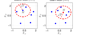
Figure 1: Motif found by searching (left) yields 3 matches while learning a latent motif (right) yields 4 matches

The frequency of a motif $M$, given a threshold $T$, can be interpreted as the number of segment points (blue in the illustration) that lies within a radius of the threshold distance from the motif (shown in red). The radius is $\sqrt{T}$ because we used the squared-Euclidean distance in Equation 2, however this poses no problems since $T$ is anyway a hyper-parameter of our method. The most frequently occurring motif is defined to be the point that covers the maximum number of blue points (segments) inside the circle of radius $\sqrt{T}$ that is centered at the motif, hence the densest geometrical ball [15]. The best segment-motif is shown in the left plot of Figure 1 and has a frequency of three. However, the optimal motif is located in the right plot and has a frequency of four. As clearly seen, the optimal solution is hidden in the space of real numbers, outside the very restricted set of segment points. The method proposed in this paper learns optimal motifs lying in the real-numbers space through a tailored numerical optimization technique. Even though the aforementioned 2-dimensional example was created to awake the reader on the need for learning motifs, still empirical results of Section 6.2 will demonstrate that learning motifs yields more frequently occurring patterns, compared to searching them, on real-life time series.

4.2 Smooth (Differentiable) Motif Frequency

We are going to find the optimal motif through a mathematical maximization of the frequency as a function of the motifs. Unfortunately, the frequency of Equation 1 has two problems (i) it is not continuous at point $||M_{k,:}-S_{j,:}||=T$ and (ii) first derivative is zero in all other points (i.e. frequency is flat having values 1 or 0). Therefore we cannot compute the optimal motifs using gradient-based optimization. However, we can use a differentiable approximation for the frequency function using the Gaussian kernel of Equations 4-5.

$$\hat{\mathcal{F}}(M) = \frac{1}{KJ}\sum_{k=1}^{K}\sum_{j=1}^{J}\hat{\mathcal{F}}_{k,j}$$ (4)

$$\hat{\mathcal{F}}_{k,j} = e^{-\frac{\alpha}{T}\sum_{l=1}^{L}\left(M_{k,l}-S_{j,l}\right)^{2}}$$ (5)

The smooth frequency function of Equation 5 is both an accurate approximation to the frequency measure from Equation 2, but also a differentiable alternative, as illustrated in Figure 2 (left plot). The parameter $\alpha$ controls the smoothness of the soft frequency. For optimization reasons (details in Section 4.4) the frequency sum of Equation 4 is divided by $KJ$ to limit the value of $\hat{\mathcal{F}}$ between 0 and 1. In terms of notation, the approximated frequency is distinguished by a hat ($\mathcal{F}$ vs $\hat{\mathcal{F}}$).

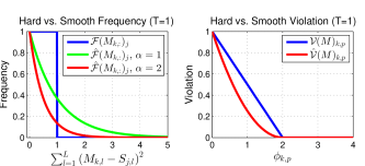
Figure 2: Smooth vs. Hard Variants of Frequency (left) and Diversity Violation (right)

4.3 Motif Diversity Violation

As previously described in Equation 3.2.1 the motifs need to be distant by a margin of $2T$. We call such a property as motif diversity. In that line, this section is devoted to formalizing a differentiable penalty function for the violations of the distances among motifs from the diversity threshold of $2T$. As a first step, the distance between two motifs $M_{k,:}\in{\mathbb{R}}^{L}$ and $M_{p,:}\in{\mathbb{R}}^{L}$ is defined as $\phi_{k,p}:\left({\mathbb{R}}^{L}\times{\mathbb{R}}^{L}\right)\rightarrow{\mathbb{R}}$ and formalized in Equation 6.

$$\phi_{k,p}=\sum_{l=1}^{L}\left(M_{k,l}-M_{p,l}\right)^{2}$$ (6)

The distance $\phi_{k,p}$ of any pair of motifs $M_{k,:},M_{p,:}$ should obey to the diversity constraint shown in Equation 7.

$$\phi_{k,p}>2T,\;\;\;\forall k\in(\{1,\dots,K\},\;\forall p\in\{k+1,\dots,K\})$$ (7)

We introduce the concept of diversity violation by Equations 8-9. For each of the $\frac{K(K-1)}{2}$ pairs of motifs, the violation is 0 if the distance between the pair motifs is greater than $2T$. Otherwise, if the distance is zero then the motifs are identical (hence not at all diverse) and a maximum violation of one is returned. For all the distances between $0$ and $2T$ a linear violation between 0 and 1 is returned as formalized in Equation 9. The constant term $\frac{2}{K(K-1)}$ makes sure that the violation function has a range between 0 and 1, the same range as the approximative frequency.

$$\mathcal{V}(M) = \frac{2}{K(K-1)}\sum_{k=1}^{K}\sum_{p=k+1}^{K}\mathcal{V}_{k,p}$$ (8)

$$\mathcal{V}_{k,p} = \begin{cases}1-\frac{\phi_{k,p}}{2T}&\phi_{k,p}<2T\\ 0&\phi_{k,p}\geq 2T\end{cases}$$ (9)

Despite achieving its aim, the violation penalty of Equations 8-9 still it suffers in terms of differentiability at the point $\phi_{k,p}=2T$. Therefore, we are proposing a smooth and differentiable variant of the violation penalty in Equations 10-11 by squaring the hard violation of Equation 9.

$$\hat{\mathcal{V}}(M) = \frac{2}{K(K-1)}\sum_{k=1}^{K}\sum_{p=k+1}^{K}\hat{\mathcal{V}}_{k,p}$$ (10)

$$\hat{\mathcal{V}}_{k,p} = \begin{cases}\left(1-\frac{\phi_{k,p}}{2T}\right)^{2}&\phi_{k,p}<2T\\ 0&\phi_{k,p}\geq 2T\end{cases}$$ (11)

As in the case of the frequency, we denote the smooth approximative version of the violation penalty by a hat ($\mathcal{V}$ for hard and $\hat{\mathcal{V}}$ for smooth). The violation penalty as a function of the distance between motif pairs is depicted in the right plot of Figure 2.

4.4 Motif Learning Through Optimization

This section fuses the smooth motif frequency and smooth motif diversity violation into a meaningful objective function. Our aim is to learn a set of $K$ motifs that maximize the frequencies and minimize (have no) violations. Such an objective can be elegantly constructed as the maximization task of Equation 12.

$$M^{*} = \operatorname*{\operatorname{argmax}}_{M}\;\;\mathcal{O}(M)$$ (12)

$$= \operatorname*{\operatorname{argmax}}_{M}\;\;\hat{\mathcal{F}}(M)-\hat{\mathcal{V}}(M)$$

The universally optimal motifs are those which achieve the universal maximum value of our objective function $O(M)=\hat{\mathcal{F}}(M)-\hat{\mathcal{V}}(M)$. As both terms are positive, the objective is maximized for the highest motif frequencies and zero violations. In this paper we will optimize the objective function through gradient ascent motif updates in a series of iterations. Since both ranges of $\hat{\mathcal{F}}$ and $\hat{\mathcal{V}}$ are between 0 and 1, no term over-scales the other and the overall learning does converge. In our preliminary experiments we found out that a trade-off coefficient $\beta$ in the form $\hat{\mathcal{F}}(M)-\beta\hat{\mathcal{V}}(M)$ was not needed as both terms converge quickly.

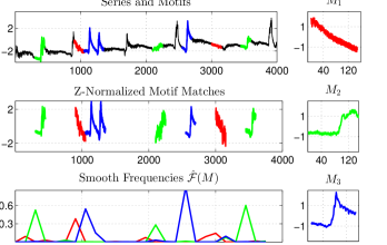
Figure 3: Top-3 motifs from the "Insect B" time series $(L=150,T=61,\eta=0.3,I=300,\alpha=2)$

The output of the learning process is a set of motifs $M$, as shown in Figure 3 for the "Insect B" time series. In this illustration the top three motifs $(K=3)$ are shown on the right plots, while the matches of the motifs on the time series are shown in the upper-left plot. Z-normalized versions of the matched segments are shown in the middle-left plot and the lower-left plot illustrates the per-segment smooth frequency scores of the motifs.

4.4.1 Gradient Ascent Optimization

Since the objective function of Equation 12 is a subtraction of frequency and diversity violations, the partial gradient of the objective function with respect to each point $l$ of any $k$-th motif is decomposable as shown in Equation 13.

$$\frac{\partial\mathcal{O}(M)}{\partial M_{k,l}} = \frac{\partial\hat{\mathcal{F}}(M)}{\partial M_{k,l}}-\frac{\partial\hat{\mathcal{V}}(M)}{\partial M_{k,l}}$$ (13)

The partial derivative of the smooth frequency with respect to the motif is computed as the first derivative of Equation 4 in terms of $M$ and shown below in Equation 14.

$$\frac{\partial\hat{\mathcal{F}}(M)}{\partial M_{k,l}} = \frac{-2\alpha}{KJT}\sum_{j=1}^{J}\left(M_{k,l}-S_{j,l}\right)\hat{\mathcal{F}}_{k,j}$$ (14)

Similarly the partial derivative of the diversity violation with respect to each motif’s point is defined in Equation 15.

$$\frac{\partial\hat{\mathcal{V}}(M)}{\partial M_{k,l}} = \frac{2}{K(K-1)}\sum_{q=1}^{K}\frac{\partial\hat{\mathcal{V}}_{k,q}}{\partial M_{k,l}}$$ (15)

$$\frac{\partial\hat{\mathcal{V}}_{k,q}}{\partial M_{k,l}} = \begin{cases}\frac{\left(\phi_{k,q}-2T\right)\left(M_{k,l}-M_{q,l}\right)}{T^{2}}&\phi_{k,q}<2T\\ 0&\phi_{k,q}\geq 2T\end{cases}$$

4.5 Learning Algorithm

Having defined the partial derivative needed for gradient ascent, we can present the complete learning method. Our method is detailed in Algorithm 2 and in this section we will explain the steps of the algorithm in detail. There are a set of hyper-parameters to the learning process, starting with the frequency smoothness $\alpha$. The other important hyper-parameters are the number of motifs $K$, the threshold $T$ and the motif length $L$, to be set by a practitioner. The learning rate $\eta$ and the number of iterations $I$ are less critical hyper-parameters that control the number of steps needed until convergence. For small learning rates and large number of iterations, the convergence is safely achievable.

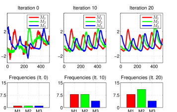
Figure 4: Metamorphosis of three motifs on the "EOG" time series $(L=150,T=58,\eta=0.3,I=300,\alpha=2)$

Algorithm 2 LearnMotifs()

1:  Input: Threshold $T\in{\mathbb{R}}^{+}$, Motif length $L\in{\mathbb{N}}^{+}$, Number of Motifs $K\in{\mathbb{N}}^{+}$, Segments $S\in{\mathbb{R}}^{J\times L}$, Learning Rate $\eta\in{\mathbb{R}}^{+}$, Number of iterations $I\in{\mathbb{N}}^{+}$, Smoothness $\alpha\in{\mathbb{R}}^{+}$

2:  Output: Motif $M\in{\mathbb{R}}^{K\times L}$

3:  // Initialize random motifs and gradient accumulators:

4:  $M\leftarrow{\left(S_{\mathcal{U}(1,J),:}\right)}^{K},\nabla\leftarrow 0^{K\times L}$

5:  // Initialize constant values:

6:  $c_{\hat{\mathcal{V}}}\leftarrow\frac{2}{K(K-1)T^{2}},\;\;c_{\hat{\mathcal{F}}}\leftarrow\frac{-2\alpha}{KJT}$

7:  // Iterate the learning method:

8:  for iter$=1,\dots,I$ do

9:     // Precompute the per-segment occurence scores:

10:     $\hat{\mathcal{F}}_{k,j}\leftarrow e^{-\frac{\alpha}{T}\sum_{l=1}^{L}\left(M_{k,l}-S_{j,l}\right)^{2}}\;\;\;\forall k\in{\mathbb{N}}_{1}^{K},\forall j\in{\mathbb{N}}_{1}^{J}$

11:     // Precompute the pair-wise motif distances:

12:     $\phi_{k,q}\leftarrow\sum\limits_{l=1}^{L}\left(M_{k,l}-M_{q,l}\right)^{2},\;\;\;\forall k\in{\mathbb{N}}_{1}^{K},\forall q\in{\mathbb{N}}_{1}^{K}$

13:     // Update the motifs :

14:     for $k=1,\dots,K;\;\;l=1,\dots,L$ do

15:        // Gradient of frequency w.r.t. the motif:

16:        $\frac{\partial\hat{\mathcal{F}}(M)}{\partial M_{k,l}}=c_{\hat{\mathcal{F}}}\sum\limits_{j=1}^{J}\left(M_{k,l}-S_{j,l}\right)\hat{\mathcal{F}}_{k,j}$

17:        // Gradient of diversity violation w.r.t. the motif:

18:        $\frac{\partial\hat{\mathcal{V}}(M)}{\partial M_{k,l}}=c_{\hat{\mathcal{V}}}\sum\limits_{q=1}^{K}\begin{cases}\left(\phi_{k,q}-2T\right)\left(M_{k,l}-M_{q,l}\right)&\phi_{k,q}<2T\\ 0&\phi_{k,q}\geq 2T\end{cases}$

19:        // Gradient of the final objective w.r.t. the motif:

20:        $\frac{\partial\mathcal{O}(M)}{\partial M_{k,l}}\leftarrow\frac{\partial\hat{\mathcal{F}}(M)}{\partial M_{k,l}}-\frac{\partial\hat{\mathcal{V}}(M)}{\partial M_{k,l}}$

21:        // Update the history of gradients:

22:        $\nabla_{k,l}\leftarrow\nabla_{k,l}+\left(\frac{\partial\mathcal{O}(M)}{\partial M_{k,l}}\right)^{2}$

23:        // Update the motif point:

24:        $M_{k,l}\leftarrow M_{k,l}+\frac{\eta}{\sqrt{\nabla_{k,l}}}\frac{\partial\mathcal{O}(M)}{\partial M_{k,l}}$

25:     end for

26:  end for

27:  return $M$

The algorithm starts with a set of motifs initialized from random segments and updates them in the direction of the partial gradients using a learning rate step size. The learning rate is dynamically updated per each point of each motif using an adaptive technique known as AdaGrad [9]. We accumulate the square of the partial gradients into accumulators denoted by $\nabla$. In order to speed-up the updates we pre-compute the per-segment frequencies $\hat{\mathcal{F}}_{k,j}$ and pair distances $\phi_{k,q}$ in lines 9-12. Then every point of each motif $M_{k,l}$ is updated in the positive direction of the derivative in lines 13-25. The partial gradients correspond to the ones previously explained in Section 4.4.1. The update of line 24 adjusts the learning rate by the square root of the accumulated square gradients [9].

As a consequence of the gradient ascent updates, the motifs undergo a metamorphosis as is shown in Figure 4 for the "Full EOG" time series. The illustrative motifs are learned on the first 10000 non-overlapping segments of the time series having length $L=150$. At the beginning (Iteration 0) the motifs are random and the corresponding frequencies zero, however the motifs start to take form after approximately 20 iterations and converge after 40 iterations. The metamorphosis of the motifs is conducted such that their matching frequencies (lower plots) are maximized.

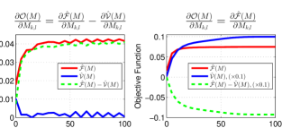
Figure 5: Convergence on "Insect B" dataset ($K=5,T=382,\eta=0.3$)

4.6 Convergence of The Learning Algorithm

The learning algorithm converges by updating the motifs so that the approximative frequency is maximized and the diversity violations minimized to zero as shown in Figure 5 (left plot) for an execution on the "Insect B" dataset. It is worth noting that the inclusion of the penalty on the diversity violation is crucial for preserving the diversity constraint. An experiment is shown on the right plot of Figure 5. In this experiment the line 24 of Algorithm 2 is edited so the motifs are updated only with respect to the frequency and not diversity violation (see plot title). As we can clearly see, maximizing the frequencies without penalizing diversity violations causes the motifs to be similar to each other. That is demonstrated by the fact that the violation measure increases, as shown in the right plot of Figure 5.

5 Optimality of Our Method

The objective function of Equation 12 is not concave, because the frequency function is a sum of Gaussians and not concave. We demonstrate the non-concavity of the frequency function in Figure 6 using the TAO and EEG LSF5 datasets. Here we generate all possible motifs of length 500 using two values, (for the sake of a 3d-plot), one value for all the first 250 points in X-axis and another value for the last 250 points in the Y-axis. As can be clearly seen, frequency is not a concave function in terms of motifs and has multiple local maxima.

Figure 6: Non-concave frequency $\hat{\mathcal{F}}(M)$ as a function of motif values $M_{1,:}$ on TAO and EEG LSF5 time-series datasets, Parameters: $L=500,T=100,\alpha=2$

In case of non-concave functions (or non-convex for minimization problems), an effective cook-book solution is to combine gradient descent with a random-restart strategy [16]. In order to avoid getting stuck in local maxima, the gradient descent optimization is restarted multiple times with random initial values for the motifs. The run that achieves the highest $\mathcal{F}(M)$ is selected, as is formalized in Equation 5, where the number of restarts is denoted by $R\in{\mathbb{N}}$. It is important to recognize that we select the motifs yielding the highest hard frequency $\mathcal{F}$, not the proxy smooth one $\hat{\mathcal{F}}$. The hard frequency $\mathcal{F}$ does avoid counting trivial matches in our implementation.

$$M^{*} := \operatorname*{\operatorname{argmax}}_{M^{(r)},\;r={1,\dots,R}}\mathcal{F}(M^{(r)})$$

$$s.t. M^{(r)}\leftarrow\text{LearnMotif() from Alg~{}\ref{alg:learnMultipleMotifs}}$$

Figure 7 illustrates the effect of 50 random restarts on the frequency function $\mathcal{F}(M)$ values over the TAO dataset. On the left plot we see that the maximum values of the objective are reached after a few restarts. The distribution of the frequency values, shown in the right plot, demonstrates that the histogram is normally distributed. That means there is a normal probability that a restart will yield an optimal value on the right portion (maximal) of the values within.

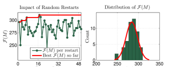
Figure 7: Impact of Random Restarts on $\mathcal{F}(M)$; "TAO" time-series dataset with hyper-parameters $L=500,K=10,\eta=0.3,I=300,T=109.6$

5.1 Runtime Algorithmic Complexity

The runtime complexity of Algorithm 2 is determined by the pre-computation steps and the update steps. Computing of the frequency terms has an algorithmic complexity order of $\mathcal{O}(RIKJL)$, while computing the pairwise distances has a computational complexity of $\mathcal{O}(RIK^{2}L)$. The computation of the partial gradients of the frequency with respect to the motifs has a complexity of $\mathcal{O}(RIKJL)$. Similarly the complexity of computing the gradients of the diversity violation with respect to the motif has a complexity of $\mathcal{O}(RIK^{2}L)$. The overall complexity of the algorithm is $\mathcal{O}(RIKJL+RIK^{2}L+RIKJL+RIK^{2}L)$, which translates to $\mathcal{O}(2RIK\left(J+K\right)L)\sim\mathcal{O}(RIKJL)$ since $K<<J$. The brute force search on the other hand, has a complexity of $\mathcal{O}(J^{2}L)$ which is quadratic in terms of the number of segments $J$. In contrast our method is linear in terms of the number of segments $J$ and faster than the brute-force search in case $RIK<J$. It is worth reminding that our algorithm learns optimal motifs (brute-force finds non-optimal motifs) and the primary strength is quality at a feasible runtime.

6 Empirical Results

6.1 Experimental Setup

We compare the quality of the proposed methods against the brute-force search strategy using a battery of six time-series datasets from diverse application domains. In addition, we employ an evaluation protocol which compares the frequencies of the computed motifs per different number of motifs, motif lengths and distance thresholds.

6.1.1 Datasets

• Insect B is a time series of insect behavior data and has a length of 73929 points [23].

• TAO is a long time series representing Tropical Atmosphere Ocean temperature measurements having 741528 measurements.

• RandomWalk is a time-series dataset consisting of 1000000 points, among which motifs at randomly selected time-stamps are implanted [23].

• EEG is a series of 1802136 continuous measurements from electroencephalographic sensors, measuring voltage differences across the scalp [23].

• Salinity is a time series containing recordings on the level of oceanic salt concentration. The data has a length of 2324134 points and is provided by the National Oceanographic Data Center.

• EOG is the longest series in our collection consisting of 8099500 points. The data is collected by an Electro-Oculogram and represent electrical potential between the front and the back of a human eye [11].

6.1.2 Baseline

Many motif discovery method are based on searching for frequent patterns among the series segments (e.g. [25, 28, 7, 14, 13], enumerated in a broader scope in Section 2). While those search-based methods are successful in terms of scalability, data representation, on-line learning, etc…, they are still upper bounded in quality (a.k.a. frequency) by the Brute-Force search. That is trivial to show, because all the frequent sub-sequences those methods could find are also detectable by Brute-Force search. In that aspect, it is sufficient to demonstrate that our method is superior to Brute-Force searching in terms of quality (a.k.a. frequency) and that naturally translates into qualitative superiority against all the other scalable/approximate/on-line search-based methods.

6.1.3 Evaluation Protocol

We will compare against the brute-force search algorithm as the most qualitative search-based baseline. Our protocol involves comparisons across all the parameters of both the searching- and learning- based methods.

Three different number of motifs will be computed $K\in\{3,10,30\}$ having two different lengths $L\in\{500,1000\}$. Furthermore, the threshold $(T)$ of the experiments is chosen as a percentile in the distribution of distances between segments. To illustrate the setup, a length corresponding to the 1%-th percentile, (denoted $\text{Pct}=1$ in Table 1) means that 1-% of segments pairs have a pairwise Euclidean distance smaller than the threshold. In that way we can compare our method against the brute-force search across a range of thresholds computed by different percentiles $T\in\{0.001\%,0.01\%,0.1\%,1\%\}$ of the pairwise distances of segments. In that way we avoid hand-picking different thresholds values per dataset and select the threshold in a data-driven neutral manner. In order to ensure convergence, the learning rate was set to an initial value of $\eta=0.1$ and the number of iterations to $I=1000$. In addition, the optimization was restarted $R=200$ times. The segments were extracted from the series by sliding a window and normalizing the clipped segment, while the window is slid by half of the motif length. For every combination of the number of motifs $K$, length $L$ and threshold $T$ (computed from the percentile), three different values of frequency smoothness were searched $\alpha\in\{1,2,3\}$, keeping the one yielding the highest $\mathcal{F}$ value.

The brute-force search baseline was executed using the same $K,L,T(\text{Pct})$ combination parameters as the learning-based approach, and for both methods the final frequency $\mathcal{F}$ does not include trivial matches. In order to be entirely transparent to the research community we publicly shared our source code and the data used in this paper in an on-line repository.

6.2 Results

Table 1: Hard Frequencies ($\mathcal{F}(M)$): Learning Motifs (LM) vs. Brute Force Motifs (BFM)

	L=500								L=1000
	Pct=0.001		Pct=0.01		Pct=0.1		Pct=1		Pct=0.001		Pct=0.01		Pct=0.1		Pct=1
	BFM	LM	BFM	LM	BFM	LM	BFM	LM	BFM	LM	BFM	LM	BFM	LM	BFM	LM
Datasets	Top-3 (K=3)								Top-3 (K=3)
Insect B	4	9	6	10	16	45	44	151	4	11	4	13	9	27	19	51
TAO	12	24	29	45	86	119	313	429	10	12	18	35	56	98	219	284
RandomWalk	25	43	74	125	239	321	697	855	9	23	27	64	114	165	327	458
EEG LSF5	17	42	47	101	150	199	388	442	11	34	27	73	96	125	232	238
Salinity	39	48	151	184	497	590	1462	1718	18	32	72	94	269	330	683	876
EOG	153	190	504	669	1646	2168	4957	8042	67	102	196	340	676	1390	2171	5998
Datasets	Top-10 (K=10)								Top-10 (K=10)
Insect B	11	18	14	23	35	78	81	189	11	29	11	28	17	54	46	97
TAO	30	48	62	95	192	314	780	1164	18	29	44	55	112	203	344	584
RandomWalk	40	79	132	206	313	579	1314	1502	23	48	52	118	223	310	603	768
EEG LSF5	42	109	131	273	400	557	1118	1266	32	96	84	212	234	379	634	810
Salinity	100	105	291	358	1000	1149	2797	2995	47	59	136	198	456	597	1222	1564
EOG	263	283	973	1296	3128	4130	11181	13439	122	164	417	685	1552	2206	4321	5729
Datasets	Top-30 (K=30)								Top-30 (K=30)
Insect B	31	40	36	47	68	107	200	221	32	49	32	49	42	72	89	110
TAO	65	95	133	209	432	698	1720	2193	38	55	65	93	202	336	577	932
RandomWalk	61	117	158	279	471	764	1778	2249	45	87	83	174	256	421	989	1151
EEG LSF5	110	281	275	646	850	1442	2541	3505	72	205	153	428	417	879	1304	1914
Salinity	162	199	428	540	1260	1456	3270	3855	91	107	233	284	660	779	2038	2150
EOG	427	557	1494	2028	5200	5681	17442	17075	247	338	787	1186	2306	2955	6227	7349
Wins	0	18	0	18	0	18	1	17	0	18	0	18	0	18	0	18

In the conducted experiments, for all the different thresholds $T$ (computed through the percentile), for all the different number of motifs $K$ and for different motif lengths $L$, the motifs learned through our method almost always had a higher frequency than the ones found through brute-force search. Table 1 displays the empirical results comparing the frequency score of the optimal learned motif (denoted $LM$) against the motifs found through brute-force search (denoted $BFM$).

The results of Table 1 indicate that learning the motifs (LM) is better than searching (BFM) them in $\bf 99.31\%$ of the experiments (143/144). The improvement arising from learning motifs (LM) in terms of motif frequencies is in average $67\pm 56\%$ better than the search-based approach (BFM). The famous Bland-Altman plot is used to assess the significance of the improvements. Figure 8 (left plot) shows the dominating ratio of LM through least-squares fitting. Moreover, the right plot shows that the difference LM-BFM and its standard deviations are above zero, thus we have a significant difference in terms of frequencies.

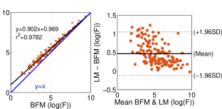
Figure 8: Bland-Altman plot showing significance of LM vs BFM frequencies (log-scale for visual comprehension)

Even though the proposed method is significantly better in quality that the search-based alternatives, it is not the fastest method in the literature (which we never claimed). Yet, it is feasible in terms of run-time, since learning the Top-30 motifs of Insect_B (smallest dataset) took 4.7 minutes, while learning the Top-30 motifs of EOG (largest dataset) took 33.57 hours, in a cluster having Intel Xeon E5-2670v2 processors with speed 2.50GHz.

7 Case Study: Audio Motifs

In this case study we extract motifs from audio files. The case discussed in this thread is a poem by Edgar Allen Poe, titled "The Bells" and famous for its onomatopoeic nature in terms of repeating the word "Bells". We extract a time-series representation of the audio file through the first channel of the Mel-frequency cepstral coefficients (MFCC). For the sake of illustration we took the first 300000 measurements of the original WAV file, corresponding to a 68 seconds audio reading of the poem.

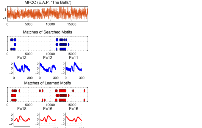
Figure 9: Learning 3 audio motifs on a read version of the "The Bells" poem from Edgar Allan Poe. The method parameters are: $T=171.56\;(Pct=0.1\%),L=300,\alpha=3,\eta=0.3,I=1000,R=4$.

Figure 9 illustrates shows the MFCC representation time-series together with the results of the brute force search algorithm in blue and our proposed method in red. We extracted three motifs $K=3$ of length $L=300$ for both methods. The distance threshold used in the experiment is the $0.1\%$-th percentile of pair-wise segment distances corresponding to a value of $T=171.56$. For each method, we display the location of the motif matches over series segments with a filled oval mark. Under the plots of the matches we show the found motifs together with the corresponding frequencies. For the same distance threshold, the learned motifs have totally $50$ matches while the searched motifs have $35$ matches, for an improvement of $42\%$ in terms of frequency. Our method learns patterns that for exactly the same distance threshold match more frequently than the brute-force motifs.

An investigation of the motif sounds reveals that the top-K repetitive sounds are different pronunciations of the word bell. All the motifs are different from each other by 2T, so they are all legit motifs by definition. Let us analyze how optimality translates in concrete terms. For instance we can consider the segment between points 10000-15000 in the times series, which corresponds to the following poem text:

… Of the rapture that impels
To the swinging and the ringing
Of the bells, bells, bells -
Of the bells, bells, bells, bells,
Bells, bells, bells -
To the rhyming and the chiming of the bells! …

Within the above segment, the brute-force motifs can find $7,10,7$ occurrences of the word bell within a threshold $T$. Our motifs can find $9,11,9$ matches within the same interval and for exactly the same distance threshold T. As the ground truth text above indicate, there are 11 "bells" pronunciations in total. In average, given the specified threshold $T$, the brute-force motifs find similar sounds that match to the word Bells in $72\%$ of the cases, the matches of our optimal motifs correspond to the word Bells in average on $88\%$ of the cases. This is a very important detection accuracy given that we used only the first channel of the MFCC representation, which is a low-resolution representation that encapsulates only the overall loudness of the sound.

8 Conclusion

This paper proposed a new perspective in learning time-series motifs. In contrast to current state of the art techniques which searches out motif candidates from series segments, our method learns them in a principled optimization. The motif frequency is approximated as a differentiable function and a gradient ascent method is proposed to find the motif values which maximize the objective function. In order to avoid local optima, a random restart strategy is combined with the gradient ascent learning of the motifs.

Learned optimal motifs have more segment matches than the motifs found through searching, for the same distance threshold. The optimal motifs represent latent patterns not necessarily present as sub-sequences in an explicit form, therefore can identify motifs which are in the center of the densest hyper-balls including segment points. Detailed experimental results demonstrate that learning optimal motifs always produces more qualitative motifs than searching them.

9 Acknowledgment

This research has been co-funded by the Seventh Framework Programme of the European Commission, through the REDUCTION project (#288254) and by Deutsche Forschungsgemeinschaft within the project HyLAP. The authors also acknowledge Prof. Eamonn Keogh, University of California, Riverside, and Dr. Lucas Drumond, ISMLL, University of Hildesheim, whose suggestions helped improving the quality of the work.

References

- [1] A. E. Brown, E. I. Yemini, L. J. Grundy, T. Jucikas, and W. R. Schafer. A dictionary of behavioral motifs reveals clusters of genes affecting caenorhabditis elegans locomotion. Proceedings of the National Academy of Sciences, 110(2):791–796, 2013.
- [2] J. Buhler and M. Tompa. Finding motifs using random projections. In Proceedings of the Fifth Annual International Conference on Computational Biology, RECOMB ’01, pages 69–76, New York, NY, USA, 2001. ACM.
- [3] N. Castro and P. Azevedo. Multiresolution Motif Discovery in Time Series. In Proceedings of the SIAM International Conference on Data Mining, SDM 2010, 2010, Columbus, Ohio, USA, pages 665–676. SIAM, 2010.
- [4] N. Castro and P. Azevedo. Time Series Motifs Statistical Significance. In Proceedings of the SIAM International Conference on Data Mining, SDM 2011, 2011, Mesa, Arizona, USA, pages 687–698. SIAM, 2011.
- [5] N. C. Castro and P. J. Azevedo. Significant motifs in time series. Stat. Anal. Data Min., 5(1):35–53, Feb. 2012.
- [6] J. Catalano, T. Armstrong, and T. Oates. Discovering patterns in real-valued time series. In J. Fürnkranz, T. Scheffer, and M. Spiliopoulou, editors, Knowledge Discovery in Databases: PKDD 2006, volume 4213 of Lecture Notes in Computer Science, pages 462–469. Springer Berlin Heidelberg, 2006.
- [7] B. Chiu, E. Keogh, and S. Lonardi. Probabilistic discovery of time series motifs. In Proceedings of the Ninth ACM SIGKDD International Conference on Knowledge Discovery and Data Mining, KDD ’03, pages 493–498, New York, NY, USA, 2003. ACM.
- [8] T. H. Cormen, C. Stein, R. L. Rivest, and C. E. Leiserson. Introduction to Algorithms. McGraw-Hill Higher Education, 2nd edition, 2001.
- [9] J. Duchi, E. Hazan, and Y. Singer. Adaptive subgradient methods for online learning and stochastic optimization. J. Mach. Learn. Res., 12:2121–2159, July 2011.
- [10] P. Ferreira, P. Azevedo, C. Silva, and R. Brito. Mining approximate motifs in time series. In L. Todorovski, N. Lavrac, and K. Jantke, editors, Discovery Science, volume 4265 of Lecture Notes in Computer Science, pages 89–101. Springer Berlin Heidelberg, 2006.
- [11] A. L. Goldberger, L. A. N. Amaral, L. Glass, J. M. Hausdorff, P. C. Ivanov, R. G. Mark, J. E. Mietus, G. B. Moody, C.-K. Peng, and H. E. Stanley. PhysioBank, PhysioToolkit, and PhysioNet: Components of a new research resource for complex physiologic signals. Circulation, 101(23):e215–e220, 2000 (June 13).
- [12] H. T. Lam, N. D. Pham, and T. Calders. Online Discovery of Top-k Similar Motifs in Time Series Data, chapter 86, pages 1004–1015.
- [13] Y. Li and J. Lin. Approximate variable-length time series motif discovery using grammar inference. In Proceedings of the Tenth International Workshop on Multimedia Data Mining, MDMKDD ’10, pages 10:1–10:9, New York, NY, USA, 2010. ACM.
- [14] Y. Li, J. Lin, and T. Oates. Visualizing variable-length time series motifs. In Proceedings of the Twelfth SIAM International Conference on Data Mining, Anaheim, California, USA, April 26-28, 2012., pages 895–906. SIAM / Omnipress, 2012.
- [15] Z. Liu, J. Yu, X. Lin, H. Lu, and W. Wang. Locating motifs in time-series data. In T. Ho, D. Cheung, and H. Liu, editors, Advances in Knowledge Discovery and Data Mining, volume 3518 of Lecture Notes in Computer Science, pages 343–353. Springer Berlin Heidelberg, 2005.
- [16] M. Lones. Sean luke: essentials of metaheuristics. Genetic Programming and Evolvable Machines, 12(3):333–334, 2011.
- [17] D. Minnen, C. Isbell, I. Essa, and T. Starner. Detecting subdimensional motifs: An efficient algorithm for generalized multivariate pattern discovery. In Proceedings of the 2007 Seventh IEEE International Conference on Data Mining, ICDM ’07, pages 601–606, Washington, DC, USA, 2007. IEEE Computer Society.
- [18] D. Minnen, C. L. Isbell, I. Essa, and T. Starner. Discovering multivariate motifs using subsequence density estimation and greedy mixture learning. In Proceedings of the 22Nd National Conference on Artificial Intelligence - Volume 1, AAAI’07, pages 615–620. AAAI Press, 2007.
- [19] Y. Mohammad and T. Nishida. Exact discovery of length-range motifs. In N. Nguyen, B. Attachoo, B. Trawiński, and K. Somboonviwat, editors, Intelligent Information and Database Systems, volume 8398 of Lecture Notes in Computer Science, pages 23–32. Springer International Publishing, 2014.
- [20] A. Mueen. Enumeration of time series motifs of all lengths. 2013 IEEE 13th International Conference on Data Mining, 0:547–556, 2013.
- [21] A. Mueen and E. Keogh. Online discovery and maintenance of time series motifs. In Proceedings of the 16th ACM SIGKDD International Conference on Knowledge Discovery and Data Mining, KDD ’10, pages 1089–1098, New York, NY, USA, 2010. ACM.
- [22] A. Mueen, E. Keogh, and N. Bigdely-Shamlo. Finding time series motifs in disk-resident data. In Proceedings of the 2009 Ninth IEEE International Conference on Data Mining, ICDM ’09, pages 367–376, Washington, DC, USA, 2009. IEEE Computer Society.
- [23] A. Mueen, E. J. Keogh, Q. Zhu, S. Cash, and M. B. Westover. Exact discovery of time series motifs. In Proceedings of the SIAM International Conference on Data Mining, SDM 2009. SIAM, 2009.
- [24] T. Oates. Peruse: An unsupervised algorithm for finding recurring patterns in time series. In Data Mining, 2002. ICDM 2003. Proceedings. 2002 IEEE International Conference on, pages 330–337, 2002.
- [25] P. Patel, E. Keogh, J. Lin, and S. Lonardi. Mining motifs in massive time series databases. In Proceedings of the 2002 IEEE International Conference on Data Mining, ICDM ’02, pages 370–, Washington, DC, USA, 2002. IEEE Computer Society.
- [26] Z. Syed, C. Stultz, M. Kellis, P. Indyk, and J. Guttag. Motif discovery in physiological datasets: A methodology for inferring predictive elements. ACM Trans. Knowl. Discov. Data, 4(1):2:1–2:23, Jan. 2010.
- [27] A. Vahdatpour, N. Amini, and M. Sarrafzadeh. Toward unsupervised activity discovery using multi-dimensional motif detection in time series. In Proceedings of the 21st International Jont Conference on Artifical Intelligence, IJCAI’09, pages 1261–1266, San Francisco, CA, USA, 2009. Morgan Kaufmann Publishers Inc.
- [28] D. Yankov, E. Keogh, J. Medina, B. Chiu, and V. Zordan. Detecting time series motifs under uniform scaling. In Proceedings of the 13th ACM SIGKDD International Conference on Knowledge Discovery and Data Mining, KDD ’07, pages 844–853, New York, NY, USA, 2007. ACM.
- [29] M. Yin, S. Tangsripairoj, and B. Pupacdi. Variable length motif-based time series classification. In S. Boonkrong, H. Unger, and P. Meesad, editors, Recent Advances in Information and Communication Technology, volume 265 of Advances in Intelligent Systems and Computing, pages 73–82. Springer International Publishing, 2014.
- [30] S. Yingchareonthawornchai, H. Sivaraks, T. Rakthanmanon, and C. Ratanamahatana. Efficient proper length time series motif discovery. In Data Mining (ICDM), 2013 IEEE 13th International Conference on, pages 1265–1270, Dec 2013.