The impact of latent heating on the location, strength and structure of the Tropical Easterly Jet in the Community Atmosphere Model, version 3.1: Aqua-planet simulations

Abstract

The Tropical Easterly Jet (TEJ) is a prominent atmospheric circulation feature observed during the Asian Summer Monsoon (ASM). The simulation of TEJ by the Community Atmosphere Model, version 3.1 (CAM-3.1) has been discussed in detail. Although the simulated TEJ replicates many observed features of the jet, the jet maximum is located too far to the west when compared to observation. Orography has minimal impact on the simulated TEJ hence indicating that latent heating is the crucial parameter. A series of aqua-planet experiments with increasing complexity was undertaken to understand the reasons for the extreme westward shift of the TEJ.

The aqua-planet simulations show that a single heat source in the deep tropics is inadequate to explain the structure of the observed TEJ. Equatorial heating is necessary to impart a baroclinic structure and a realistic meridional structure. Jet zonal wind speeds are directly related to the magnitude of deep tropical heating. The location of peak zonal wind is influenced by off-equatorial heating which is closest to it. Hence the presence of excess rainfall in Saudi Arabia has been shown to be the primary reason for the extreme westward shift of the TEJ maximum.

Keywords: Tropical Easterly Jet Indian Summer Monsoon CAM-3.1 orography aqua-planet precipitation

1 Introduction

The Tropical Easterly Jet (TEJ) is one of the most defining features of the Indian Summer Monsoon (ISM) which itself is a part of the Asian summer monsoon (ASM). The jet is observed mostly during the ISM that is in the months of June to September. It has a maximum between 50^∘E-80^∘E, Equator-15^∘N and at 150hPa. The TEJ was first discovered by Koteswaram (1958). It has a great influence on the rainfall in Africa (Hulme and Tosdevin, 1989). The correct simulation of the TEJ is important for accurate seasonal predictions and weather forecasting.

The Tropical Easterly Jet is believed to be influenced by the Tibetan Plateau. Previous studies (Flohn, 1968, Krishnamurti, 1971) have highlighted the presence of a huge upper tropospheric anticyclone above the Tibetan Plateau in summer. The origin of the Tibetan anticyclone itself has been attributed to the summertime insolation on the Tibetan Plateau. This sensible heating is widely regarded as the primary reason for this region to act as an elevated heat source. Flohn (1965) first suggested that in summer, southern and southeastern Tibet, i.e. south of 34^∘N-35^∘N, act as an elevated heat source which changes the meridional temperature and pressure gradients and contributes significantly to the reversal of high tropospheric flow during early June. Flohn (1968) showed that sensible heat source over the Tibetan Plateau as well as latent heat release due to monsoonal rains over central and eastern Himalayas and their southern approaches generates a warm core anticyclone in the upper troposphere at around 30^∘N. This was a primary mechanism for establishing the south Asian monsoonal circulation over south Asia. According to Koteswaram these winds are a part of the Tibetan Anticyclone which forms during the summer monsoon over South Asia. He believed that the southern flank of the anticyclone preserved its angular momentum and became an easterly at approximately 15^∘N. Contradicting Koteswaram, Raghavan (1973) opined that the upper tropospheric zonal component of the equatorward outflow from the Tibetan anticyclone does not agree with the law of conservation of angular momentum. However the thermal gradient balance was applicable and this was responsible for the origin of the TEJ.

The TEJ is not simply a passive atmospheric phenomena. Hulme and Tosdevin (1989) studied the impact of the TEJ on Sudan rainfall. El Niño events were suggested as a direct control over Sahelian rainfall via the TEJ. The decelerating limb of the TEJ showed interannual variations in location in relation to Eastern Pacific warming. Fluctuations in the jet were shown to be responsible for altering precipitation patterns in Sudan. Camberlin (1995) also reported on the significant linkages between interannual variations of summer rainfall in Ethiopia-Sudan region and strength and latitudinal extent of upper-tropospheric easterlies. More recently Nicholson et al. (2007) showed that the wave activity of the TEJ influences the African easterly jet (AEJ). The AEJ in turn influences the weather patterns over the Atlantic coast of Africa. Bordoni and Schneider (2008) discussed the role of TEJ in modifying the monsoonal circulation. Upper-level easterlies shield the lower-level cross-equatorial monsoonal flow (which later becomes the Somali jet) from extratropical eddies. This made the angular momentum conservation principle applicable to overturning Hadley cell dynamics. In the larger picture this implies a strengthening of the monsoonal regime. This shows that the TEJ actively shapes the climate and weather pattern in regions not under the direct influence of the Indian Summer Monsoon.

In fact the TEJ also shows intraseasonal and interdecadal variations in its location. Sathiyamoorthy et al. (2007) reported that the axis of the jet undergoes meridional movement in response to active and break phases of the Indian Monsoon. Sathiyamoorthy (2005) also observed a reduction in the spatial extent of the TEJ between 1960-1990. According to him the TEJ almost disappeared over the Atlantic and African regions. This reduction coincided with the 4-5 decade prolonged drought conditions over the Sahel region. He speculated that these two phenomena were associated with each other. This explanation also implies that latent heating significantly influences the characteristics of the TEJ.

Ye (1981) did laboratory experiments to simulate the heating effect of elevated land. He introduced heating in an ellipsoidal block resulting in vertical circulation, an anticyclone in the upper layer and a cyclonic flow in the lower layer. The pattern was found to be qualitatively similar to summer time atmospheric circulation in south Asia. Raghavan (1973) discussed the importance of Tibetan Plateau and explained that the jet owed its existence the the temperature gradients that was partly influenced by the Tibetan high. According to Wang (2006) the elevated heat source of the Tibetan Plateau was instrumental in providing an anchor to locate the Tibetan high. On the other hand Hoskins and Rodwell (1995) and Liu et al. (2007) have argued that orography plays a secondary role in determining the position of the summertime upper tropospheric anticyclone. Jingxi and Yihui (1989) studied the TEJ at 200 hPa and found that precipitation changes in the west coast of India led to changes in the jet structure. Chen and van Loon (1987) observed that at 200 hPa the jet was weaker during El Niño and Indian drought events. The TEJ was weaker in the drought years of 1979, 1983 and 1987 and stronger in the excess monsoon years 1985 and 1988.

According to Zhang et al. (2002), the South Asian High had a bimodal structure. Its two modes – one the Tibetan mode and the other the Iranian mode, both of which were fairly regular in their occurrence, were mostly influenced by heating effects. The former owed its existence to diabatic heating of the Tibetan Plateau, while the latter occurred due to adiabatic heating in the free atmosphere and diabatic heating near the surface.

Thus it can be seen that while there have been attempts in the past to explain some aspects of the TEJ and its effects, the issue about the importance of orography on the TEJ has not yet been settled. In the previous discussions variations in the jet were in the presence of the Himalayas and Tibetan Plateau. Although the importance of latent heating on the TEJ is quite clear now, it is necessary to confirm the importance of orography in deciding the location of the TEJ. It is necessary to study the jet in a GCM and understand the relative roles played by latent heating and orography on the TEJ. An Atmospheric General Circulation Model (AGCM), CAM-3.1, has been used to study the impact of orography and monsoonal heat sources on the TEJ. The jet location and its response to have been studied by:

1. Modifying the deep-convective scheme and thereby changing the monsoonal heating pattern.

2. Removing orography.

A series of aqua-planet experiments have been conducted determine the factors influencing the location, structure and strength of the TEJ in CAM-3.1.

2 The Tropical Easterly Jet in reanalysis

For wind data, NCEP (Kalnay et al., 1996) and ERA40 (Uppala et al., 2005) data have been used, and GPCP (Adler et al., 2003) and CMAP (Xie and Arkin, 1997) data for precipitation. Unless otherwise mentioned the time period chosen spans years 1980 to 2002. The maximum zonal winds occur at 150hPa. From Fig. 1 it is seen that the TEJ peaks in July to August. Hence, in present work the focus is on the TEJ during the month of July when it first reaches its maximum value.

Figure 1: Time series of 150 hPa zonal wind averaged between 50^∘E-80^∘E, Equator-15^∘N showing TEJ peaking in July-August (NCEP: 1980-2002 avg)

The magnitude of peak zonal wind and its location are listed in Table 1. Due to the good agreement between zonal winds of NCEP and ERA40, only shown the former is shown. In Fig. 2a, the zonal wind and location of peak zonal wind, henceforth $U_{max}$, for NCEP at 150hPa, is shown. The ‘cross-diamond’ indicates the horizontal location of $U_{max}$. The location of peak zonal wind of each individual year from 1980-2002 was found and then the means were calculated. The standard deviation for the zonal winds for NCEP and ERA40 was found to be 2 m s^-1 and 1.7 m s^-1 respectively. The meridional section of the zonal wind is shown in Fig. 3a. This vertical cross-section corresponds to the longitude where the zonal wind is maximum. The meridional structure shows the jet peak lying between equator and $\sim$20^∘N. A vertical equator to pole tilt towards higher pressure levels can be observed. The mean height of maximum easterly zonal wind speeds are higher at higher latitudes. In Fig. 4a the velocity vectors and geopotential high is shown. The peak is not over the Tibetan Plateau but to the west of it.

Table 1: Magnitude ( m s^-1) and location of peak zonal wind, and centroid of mean precipitation

reanalysis and observation
Case	Zonal wind				Precipitation
	Peak	Lon	Lat	Press	Lon	Lat
NCEP	34.48	65.1∘E	10.3∘N	150
ERA40	33.61	68.7∘E	10.4∘N	150
GPCP					96.0∘E	11.9∘N
CMAP					95.8∘E	10.0∘N
CAM-3.1 simulations
Case	Zonal wind				Precipitation
	Peak	Lon	Lat	Press	Lon	Lat
Ctrl	47.19	42.5∘E	8.8∘N	125	76.7∘E	9.7∘N
noGlOrog	43.45	43.5∘E	7.6∘N	125	77.0∘E	7.4∘N
Ctrl: default orography
noGlOrog: no orography

(a) NCEP (150 hPa)

(b) Ctrl (125 hPa)

(c) noGlOrog (125 hPa)

Figure 2: July horizontal zonal wind profile at pressure level where maximum zonal wind is attained, ‘cross-diamond’ is location of peak zonal wind: NCEP, Ctrl and noGlOrog.

(a) NCEP

(b) NCEP

(c) Ctrl

(d) Ctrl

(e) noGlOrog

(f) noGlOrog

Figure 3: July cross-section of zonal wind profile at the longitude (left panel) and latitude (right panel) where $U_{max}$ is attained (see Table 1 for details): NCEP, Ctrl and noGlOrog.

(a) NCEP

(b) Ctrl

Figure 4: July velocity vectors and geopotential height ($\times 10^{3}$m) at 150 hPa. ‘Cross-diamond’ is location of peak geopotential height. Contour for NCEP and Ctrl is 14.36 and 14.43 respectively which is 99.5% of individual peak.

2.1 Impact of latent heating on the location of the TEJ

The TEJ is not a stationary entity. Variations in its position in different years can also be observed. This is most strikingly observed in July 1988 and 2002. The location of the TEJ in during these two years is radically different. This is seen in Fig. 5a where the 30 m s^-1 zonal wind contour and $U_{max}$ locations show significant differences. In fact the location of $U_{max}$ is shifted eastwards by $\sim$20^∘ in 2002. These differences are seen in ERA40 data as well. The vertical structure in these two years is similar to Fig. 3a.

It is well known that in India 2002 was a drought year (Sikka, 2003, Bhat, 2006) while 1988 was an excess monsoon year. The relationship between precipitation and the jet location in the month of July for these two years is now clarified. Here in order to be self-consistent,both precipitation and zonal winds from NCEP data have been used. This is because reanalysis data is self-consistent and that the dynamic response of the atmosphere is entirely on account of forcing from the same data. If the TEJ is influenced largely by latent heating due to Indian Summer Monsoon then the July 2002 shift should be due to the mean rainfall being eastward shifted. This is clearly seen in Fig. 5b where precipitation differences between July 1988 and 2002 have been plotted. The differences are quite striking. In July 2002 there is a clear eastward shift in rainfall with the maximum being in the Pacific warm pool and relatively little in the Indian region. This is in contrast with July 1988 where Indian region received high amounts of precipitation. The jet in 1988 peaks at 60^∘E-65^∘E while in 2002 the maximum is in the southern Indian peninsula, implying a $\sim$20^∘ westward shift. The same behaviour was also found for ERA40 data and hence is not shown.

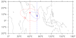
(a) NCEP zonal wind, 1988 (red), 2002 (blue)

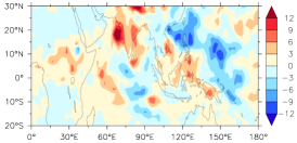
(b) NCEP precipitation difference: 1988–2002

Figure 5: LABEL:sub@nc-jul-Umax-88,02-xy 30 m s^-1 zonal wind contour (dashed) in 1988 and 2002 showing shift in TEJ in response to heating, cross-sections are at $U_{max}$ pressure level (150hPa), ‘cross-diamond’ shows the location of maximum zonal wind; LABEL:sub@nc-jul-Rdiff-xy precipitation difference ( mm day^-1), year 2002 subtracted from 1988. All data from NCEP.

3 The Tropical Easterly Jet in CAM-3.1

3.1 Description of CAM-3.1 and experiment details

The AGCM that has been used for the present work is the Community Atmosphere Model, version 3.1 (CAM-3.1). The finite-volume dynamical core using the recommended 2^∘$\times$2.5^∘ grid resolution has been used for all simulations. The time step is 30 minutes and 26 levels in the vertical are used. Deep convection is the Zhang and McFarlane (1995) scheme while shallow convection is the Hack (1994) scheme. Stratiform processes employs the Rasch and Kristjánsson (1998) scheme updated by Zhang et al. (2003). Cloud fraction is computed using a generalization of the scheme introduced by Slingo (1989). The shortwave radiation scheme employed is described in Briegleb (1992). The longwave radiation scheme is from Ramanathan and Downey (1986). Land surface fluxes of momentum, sensible heat, and latent heat are calculated from Monin-Obukhov similarity theory applied to the surface. Climatological mean SST was specified as the boundary condition. Sea surface temperatures are the blended products that combine the global Hadley Centre Sea Ice and Sea Surface Temperature (HadISST) dataset (Rayner et al., 2003) for years up to 1981 and Reynolds et al. (2002) dataset after 1981.

The model was run in its default configuration for a five year period. This simulation is referred to as the control (Ctrl) simulation. Additionally another simulation (referred to as noGlOrog) has been conducted to check the influence of orography on the TEJ. This has also been run for five years with same boundary conditions but with orography all over the globe removed. This latter simulation is used to investigate the direct influence of topography on the TEJ. All the simulation results presented in this paper are based on five year means.

3.2 Impact of orography on the simulated TEJ

The 5 year average of maximum zonal wind and its corresponding location have been computed. The horizontal (Figs. 2b,LABEL:sub@nglo-xy) and meridional (Figs. 3c,LABEL:sub@nglo-yz) profiles of the TEJ for Ctrl and noGlOrog simulations are shown. As with reanalysis, the vertical cross-section is at the location of zonal wind maximum. The existence of a Tropical Easterly Jet can be observed. In both the simulations the first noticeable feature is a $\sim$30^∘ westward shift of the simulated jet. This shift in the default Ctrl was also documented by Hurrell et al. (2006) where they analyzed the 200hPa JJA zonal wind fields. The location of the peak zonal wind is virtually the same for Ctrl and noGlOrog simulations while the jet is weaker in the absence of orography. The zonal cross-section also shows that the zero line at 500 hPa is sandwiched between the peaks in the TEJ and low-level Somali jet. One major difference appears in the Ctrl and noGlOrog simulation - the maximum in the Somali jet is greater and restricted east of $\sim$50^∘E in the former. This was explained by Chakraborty et al. (2008). The absence of orography in the latter caused the low-level wind to spread out and thereby reduce the intensity without compromising on the total flow. This is also seen in NCEP data (Fig. 3b) where the Somali jet is also maximum to the east of $\sim$50^∘E. The meridional cross-section is very similar to real-planet and shows the familiar vertical equator to pole tilt with the maximum lying between equator and $\sim$20^∘N. The depth is also maximum on the poleward side.

The impact of orography in determining the location and spatial structure of the jet in CAM-3.1 is thus minimal. The location of the peak zonal wind is virtually the same for Ctrl and noGlOrog simulations while the jet is weaker in the absence of orography. Although CAM-3.1 does show reasonable fidelity in determining the spatial features of the TEJ, the discrepancies in location and magnitude of the maximum velocity of the TEJ need to be understood. With the insight gained from section 2.1 the spatial distribution of simulated and observed rainfall is now studied.

4 Spatial distribution of heating in reanalysis and Ctrl

The westward shift of the simulated TEJ indicates that sensible heating from the Tibetan Plateau may not play a major role in the existence and location of TEJ. During the monsoon season the major source of heating in the tropics is latent heating and hence it is necessary to look at the role of latent heating.

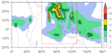
(a) Precipitation: GPCP

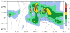
(b) Precipitation: CMAP

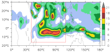
(c) Precipitation: Ctrl

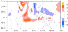
(d) Precipitation difference

Figure 6: LABEL:sub@gpcp-jul-R-xy, LABEL:sub@cmap-jul-R-xy, LABEL:sub@cc-jul-R-xy July precipitation ( mm day^-1). LABEL:sub@mix-Rdiff-xy July precipitation difference ( mm day^-1) (Ctrl–(GPCP+CMAP)/2).

Figs. 6a-LABEL:sub@cc-jul-R-xy show the precipitation in the month of July of GPCP, CMAP and Ctrl. The difference between Ctrl and mean of GPCP and CMAP is shown in Fig. 6d. The observational data have been averaged since the precipitation patterns are very similar. The contrast between reanalysis and model simulations is quite striking. Most noticeable discrepancies in model simulations are (i) significantly reduced precipitation in northern Bay of Bengal, East Asia, western Pacific warm pool (ii) a significant precipitation tongue just south of the equator between 50^∘E-100^∘E and (iii) Spurious precipitation in the Saudi Arabian region which is quite prominent and equal in magnitude to the precipitation peaks in central Arabian Sea and south-western Bay of Bengal. This implies a major realignment in the local heating pattern. This unrealistic precipitation has been discussed by Hurrell et al. (2006).

Thus from Table 1 and Fig. 6 it appears that westward shift in the peak of the simulated precipitation is responsible for the TEJ to be centered east Africa. The strongest impact seems to be from the significantly high anomalous precipitation in the Saudi Arabian region which could play a part in the extreme westward shift of the TEJ.

As in Kucharski et al. (2009) and Davis et al. (2012), precipitation is used as a proxy for latent heating. The centroid of precipitation ($P_{c}$) has been computed for in a region that is spatially quite significant and covers the monsoon region. Different regions for reanalysis and CAM-3.1 simulations have been chosen since the precipitation pattern is spatially different. For reanalysis the west Pacific warm pool is also considered, while it is ignored for model simulations. The region chosen for reanalysis is 60^∘E-130^∘E, 16^∘S-36^∘N and for the simulations it is 40^∘E-110^∘E, 16^∘S-36^∘N (region demarcated by red boxes in Figs. 6a-LABEL:sub@cc-jul-R-xy). From Table 1 it is seen that the mean precipitation in simulations and reanalysis are in reasonable agreement although Ctrl experiment overestimated the precipitation by $\sim$15%. The excess precipitation could be a cause for stronger jet speeds. The centroid of the precipitation, henceforth $P_{c}$, is computed using the following equation:

$$x_{c}=\frac{\sum_{i}{P_{i}x_{i}}}{\sum_{i}{P_{i}}},y_{c}=\frac{\sum_{i}{P_{i}y_{i}}}{\sum_{i}{P_{i}}}$$ (1)

where,
$x_{c}$ and $y_{c}$ are the zonal and meridional coordinates of the $P_{c}$,
$P_{i}$ is the precipitation at each grid point,
$x_{i}$ and $y_{i}$ are the zonal and meridional distances from a fixed coordinate system, in each case the grid point where peak precipitation occurs.

The distances are measured from a coordinate system centered at a point where the precipitation is maximum in the chosen region. There is a clear $\sim$20^∘ westward shift in the precipitation centroid in Ctrl with respect to reanalysis. Precipitation pattern of noGlOrog is similar to Ctrl and hence even in this case the shift is $\sim$20^∘ westward. The latitudinal differences are not significant. Choosing slightly different averaging regions does not significantly distort this relationship.

Consequent to the westward shift in the precipitation centroid and TEJ, the peak geopotential height at 150hPa in the simulations has also shifted westwards by $\sim$25^∘. This is clearly seen in Fig. 4 where the geopotential contour corresponds to 99.5% of the peak, the location of which is indicated by the ‘cross-diamond’. The velocity vectors clearly show the anti-cyclonic flow around the geopotential high.

Though this offers evidence of the primacy of latent heating in determining the location of the jet, the validity of this argument is further demonstrated by showing the precipitation patterns of the Ctrl$\tau_{d12}$ and noGlOrog$\tau_{d12}$ simulations. The mean precipitation and centroid are shown in Table 1. Since the precipitation pattern is now similar to real-planet (not shown), the same region as in real-planet has been used to compute the location of the precipitation centroid. Figs. 7a,LABEL:sub@nglot-xy show the precipitation and TEJ in these two simulations. The location of the TEJ agrees well with real-planet. Although the mean precipitation is more in comparison to the previous simulations, the peak zonal wind speed is almost the same. The geopotential high (Fig. 7c) in the Ctrl$\tau_{d12}$ simulation is now almost same as that in NCEP (Fig. 4a). The spatial separation between the precipitation centroid and $U_{max}$ is included in Fig. 8. The zonal separation is also in closer agreement to real-planet and this is may be attributed to the increased similarity in spatial pattern of precipitation in real-planet and these two simulations. The similarity in the precipitation patterns and TEJ structures in both these simulations as well as the previously discussed Ctrl and noGlOrog simulations suggests that it is the location and strength of the heat source and not orography that controls the TEJ. The only difference in precipitation between the Ctrl$\tau_{d12}$ and noGlOrog$\tau_{d12}$ simulations is that the former has additional heating to the north of 20^∘N around 90^∘E longitude. The absence of this peak in the latter further suggests that the Tibetan Plateau is not the primary reason to set up the temperature gradients that lead to the formation of the TEJ. Sensible heating due to the presence of Tibetan Plateau may be less important when dominated by latent heat release due to convective processes.

(a) Ctrl$\tau_{d12}$ (125 hPa)

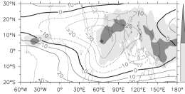
(b) noGlOrog$\tau_{d12}$ (125 hPa)

(c) Ctrl$\tau_{d12}$ (150 hPa)

Figure 7: LABEL:sub@cct-xy, LABEL:sub@nglot-xy July precipitation ( mm day^-1, shaded) and horizontal zonal wind ( m s^-1) profile at pressure level where maximum zonal wind is attained; ‘cross-diamond’ is location of peak zonal wind, LABEL:sub@cct-z3-xy velocity vectors and geopotential height ($\times 10^{3}$m) at 150 hPa; ‘cross-diamond’ is location of peak geopotential height; contour value is 14.46 which is 99.5% of peak: Ctrl$\tau_{d12}$ and noGlOrog$\tau_{d12}$.

Figure 8: Separation ($P_{c}$–$U_{l}$) between location of precipitation centroid and maximum zonal wind. ‘Cross-diamond’ denotes aqua-planet simulations, ‘plus’ denotes real-planet simulations and reanalysis.

Thus it has been demonstrated that there is a close correspondence between the source of heating, spatial location of TEJ and the geopotential high. The negligible influence of orography and strong effect of heating on upper level wind patterns has also been discussed by Liu et al. (2007). It is also worthwhile to note that the Somali jet in NCEP and Ctrl simulation is roughly in the same location and hence the lower and upper-level winds (Figs. 3b,LABEL:sub@cc-zx) are not merely reflections of each other, not just in magnitude but also in location, as simple though insightful models, e.g. Gill (1980) suggest. However the spatial location of the low-level jet and upper-level TEJ is more closely correlated in the noGlOrog simulation and this is due to the absence of orography as will also be shown in the subsequent discussion on aqua-planet simulations.

However this mean pattern does not present the full picture. Between 70^∘E-100^∘E the precipitation peak in real-planet is more northwards in comparison to CAM-3.1 while the opposite is true between 30^∘E-60^∘E. In fact real-planet hardly shows rainfall in the latter region. Hence it is not clear how the spatial structure of the precipitation influences the positioning of the TEJ. This aspect will need to be clarified before further analysis and this will be the focus of the next section where a major simplification is adopted by running CAM-3.1 in the aqua-planet (AP) mode.

5 Aqua-planet simulations

Since orography has hardly any impact on the TEJ in the real-planet simulations it is instructive to study the atmospheric response only due to heating. The multiplicity of heat sources both in reanalysis and Ctrl preclude any easy interpretation of the influence that each heat source has on the TEJ. A major simplification is conceivable if one removes orography, land, sea-ice totally and further remove seasonal cycles, and yet retain all the important physics that the AGCM offers. This also implies that one needs to prescribe SSTs as a boundary condition. All this is possible in the aqua-planet configuration of CAM-3.1. The solar insolation is perpetually fixed at 21^st March which is March Equinox.

In order to understand the role played by heating in determining the structure and location, CAM-3.1 has been run in aqua-planet configuration. The basic state consists of a uniform background SST on which additional heat sources are imposed. The heat sources are indirectly specified by setting an SST perturbation on this uniform SST background. Precipitation induced on account of this SST perturbation is representative of total atmospheric heating. The implicit assumption is that latent heating is the dominant effect in the region of precipitation.

The rationale for imposing heat sources on a uniform SST background in contrast to a zonally symmetric and meridionally varying SST profile is now explained. Rajendran et al. (2013) showed that equatorial easterlies will be simulated even if a zonally symmetric but meridionally varying SST profile, symmetric about the equator, is used. The existence of an equatorial jet also depends on the presence of twin or single Inter-Tropical Convergence Zone (Rajendran et al. (2013), Neale and Hoskins (2001)). In such a meridionally varying SST profile it is more difficult to determine the role played by weak heat sources in the formation of a jet in aqua-planet.

The aqua-planet simulations with just uniform background SSTs of 20^∘C and 25^∘C had a weak equatorial easterly of about 10-15 m s^-1 peaking at $\sim$250hPa. In this simple configuration, it is implicitly assumed that SSTs beyond 60^∘N/^∘S do not significantly influence equatorial dynamics. This was also suggested by Hoskins and Rodwell (1995) when they conducted a series of experiments to understand the Asian summer monsoon. Thus a uniform background SST is deemed to be the simplest basic state on which additional heating may be imposed to study the influence of heating on the TEJ.

The reasons for the existence of these easterlies is as follows: these simulations had a band of weak precipitation near the equator. This would naturally imply that moist parcels arise aloft implying the presence of a weak Hadley Cell. This means that air is mixed latitudinally. Therefore there must be westerly motion at higher latitudes and easterly motion at lower latitudes owing to angular momentum conservation. The time-averaged torque on the whole atmosphere due to surface friction must be zero, which requires that there be both easterly and westerly winds. Thus easterlies must prevail near the equator. Drag on surface easterlies also transfers angular momentum from the surface to the atmosphere (Schneider (2006)). The issue of the existence of equatorial upper tropospheric easterlies has also been discussed by Lee (1999). According to her, in the deep tropics the horizontal transient eddy momentum flux accelerates the zonal mean zonal wind. Transient eddies of intraannual and interannual timescales were important determining factors. Hadley cell dynamics was also important. According to Bordoni and Schneider (2008) the Hadley cell approaches the angular momentum conservation limit because of these upper-level easterlies (upper-level easterlies strengthen when additional off-equatorial heating is present).

The details of all the aqua-planet simulations are in Tables 2 and 3. In Fig. 9, the different locations where SSTs are imposed are shown. The names of the aqua-planet simulations start with ‘AP’. The magnitude of peak zonal wind and mean precipitation are listed in Table 3. The important point to note is that the SSTs have been chosen such that mean of precipitation exceeding 5 mm day^-1 compares well with reanalysis and real-planet simulations. Fig. 8 shows the zonal and meridional distance between $P_{c}$ and $U_{max}$. Equation (1) has been used to compute the centroid. The zonal wind for each month has not been individually computed and then averaged; the zonal find fields have been added and then averaged for the six month period. Hence these locations correspond to grid point values of the model. This method is acceptable since the heat source is stationary and the response too will average out over a six month time scale. The coarse model resolution implies that minor fluctuations in location will hardly distort the main observations and inferences. The vertical sections at the longitude and latitude where $U_{max}$ is attained. Some representative cases are discussed.

Figure 9: Schematic showing locations of imposed SSTs for aqua-planet simulations. Refer Table 2 for further details. (Not drawn to scale).

Table 2: Location and nomenclature of SST profiles for aqua-planet simulations. See table 3 for full nomenclature. Figure 9 shows the schematic of the locations.

Region	Shape of SST profile		Location of SST peak
S	Circle (C)	20∘ diameter	90∘E,20∘N
	Oval (Oa)	50∘ major axis
		16∘ minor axis
	Oval (Ob)	90∘ major axis
		16∘ minor axis
E	Rectangle	10∘ slope	62∘E,4∘S to 94∘E,2∘S
	Circle	20∘ diameter	60∘E,4∘N
B	Circle	20∘ diameter	50∘E,20∘N
C			70∘E,14∘N
D			85∘E,10∘N
P	Oval	As in (Ob) above	120∘E,20∘N
			150∘E,10∘N
			130∘E,2∘S

Table 3: Magnitude ( m s^-1) and location of peak zonal wind, and magnitude ( mm day^-1) and centroid of mean precipitation for aqua-planet simulations. Refer Fig. 9 and table 2 for shape and location of SST profiles.

Single heat source (at region S) simulations
Case	SST		Zonal wind				Precipitation
	Peak	Shape	Peak	Lon	Lat	Press	Mean	Lon	Lat
AP_S1	29∘C	Circle (C)	23.64	70∘E	6∘N	175	8.81	90.2∘E	21.9∘N
AP_S2	32∘C		33.97	80∘E	10∘N	150	12.41	90.5∘E	21.6∘N
AP_S3	29∘C	Oval (Oa)	30.75	65∘E	6∘N	175	9.24	88.8∘E	20.7∘N
AP_S4	32∘C		37.98	67.5∘E	6∘N	150	14.74	89.4∘E	21.4∘N
AP_S5	29∘C	Oval (Ob)	35.58	45∘E	4∘N	175	10.17	86.3∘E	20.5∘N
AP_S6	32∘C		42.56	40∘E	4∘N	150	15.06	88.6∘E	20.1∘N
Uniform background temperature: 25∘C
Multiple heat source simulations
Case	SST region	Zonal wind				Precipitation
		Peak	Lon	Lat	Press	Mean	Lon	Lat
AP_E1	E	15.54	52.5∘E	2∘N	225	11.52	74.2∘E	3.6∘S
AP_E2		17.58	37.5∘E	6∘N	225	11.49	72.5∘E	2.4∘S
AP_N1	B,C,D	33.08	37.5∘E	10∘N	150	9.02	67.7∘E	16.7∘N
AP_N2		30.41	57.5∘E	6∘N	175	9.27	72.3∘E	16.2∘N
AP_NE1	B,E	26.73	37.5∘E	8∘N	175	10.37	67.0∘E	2.7∘N
AP_NE2		23.80	42.5∘E	14∘N	150	7.51	67.3∘E	3.1∘N
AP_M1	C,D,E	30.89	55∘E	6∘N	125	11.40	70.8∘E	5.4∘N
AP_M2		24.91	52.5∘E	4∘N	150	11.62	71.6∘E	2.6∘N
AP_M3	B,C,D,E	24.31	40∘E	10∘N	150	9.03	71.9∘E	2.3∘N
AP_M4		36.02	35∘E	8∘N	150	9.03	68.7∘E	5.4∘N
AP_M5		34.43	32.5∘E	6∘N	150	10.86	69.2∘E	4.9∘N
AP_M6	B,C,D,E,P	35.70	32.5∘E	8∘N	150	10.22	68.8∘E	3.1∘N
Uniform background temperature: 22∘C					Peak temperatures: $\leq$ 29∘C

5.1 Single heat source simulations

For single heat source simulations, the SST profiles imposed have circular and oval shapes all centered at 90^∘E,20^∘N which mimic the off-equatorial monsoonal heat source in the northern Bay of Bengal. The circular profiles (AP_S1 and AP_S2) have a diameter of 20^∘ while the oval shaped profiles have major axes of either 50^∘ (AP_S3 and AP_S4) or 90^∘ (AP_S5 and AP_S6). All oval profiles have a minor axis of 16^∘. The simulations with oval-shaped SSTs serve to demonstrate the effect of the shape of the heating region on the jet. The peak SSTs are at 90^∘E,20^∘N. They go linearly down to the background temperature. However the profile with major axes of 90^∘ (AP_S5 and AP_S6) has a non-linear SST gradient which is used to study if the gradient has any qualitative change on the jet. The background temperature is 25^∘C. In each set, the first simulation in each set has 29^∘C peak SST while the second has 32^∘C peak SST. For example, AP_S3 has 29^∘C and AP_S4 has 32^∘C SST peak on a uniform background temperature of 25^∘C.

The meridional and zonal cross-sections (Figs. 10a,LABEL:sub@S6-zx) are shown for AP_S6 simulation. Meridionally, the jet is not symmetric. The major difference with reanalysis and real-planet simulations lies in the vertical shape of the jet. With single off-equatorial heat source the jet has a pole to equator tilt towards higher pressure levels. This is opposite to reanalysis and real-planet (Figs. 3a,LABEL:sub@cc-yz). Below 500 hPa, there is also a region of weak low-level jet which is the aqua-planet counterpart of the Somali jet (not shown). Further, the low-level westerly was observed to be either very weak or almost non-existent for those simulations with reduced spatial extent of heating and/or lesser overall heating rates, for example AP_S2 and AP_S5.

(a) Meridional cross-section

(b) Zonal cross-section

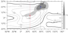
(c) Horizontal cross-section: (150 hPa)

(d) Velocity vectors and geopotential height

Figure 10: Zonal wind ( m s^-1) profile. Vertical sections are at the LABEL:sub@S6-yz longitude and LABEL:sub@S6-zx latitude where $U_{max}$ is attained; LABEL:sub@S6-xy horizontal cross-section at pressure level where $U_{max}$ is attained, ‘cross-diamond’ is location of $U_{max}$, ‘star’ is location of $P_{c}$, precipitation contours ( mm day^-1) are shaded; LABEL:sub@S6-z3-xy velocity vectors and geopotential height ($\times 10^{3}$m) at 150 hPa; ‘cross-diamond’ is location of peak geopotential height; contour value is 14.09 which is 99.5% of peak: AP_S6 (Aqua-planet with single off-equatorial heat source in region S shown in Fig. 9).

To the east of the jet, there is an upper-level westerly intrusion. A hint of this westerly is also observed in the reanalysis and real-planet simulations (Fig. 3, right panel). In Fig. 10c, the precipitation region is demarcated by the 5 mm day^-1 and above shaded contours. It can be seen that precipitation (also refer Table 3) for the AP_S6 case has very high rates which is unrealistic. For comparatively low heating rates, a baroclinic structure similar to reanalysis and real-planet simulations does not exist. This only suggests that for such cases, the easterlies developed are more of an add-on to the equatorial easterlies developed with uniform background SSTs. However even low heating more than doubles the peak zonal winds generated in comparison to only uniform SST everywhere. This shows that even relatively higher zonal easterly wind speeds may not create vertical structures that have any resemblance with reanalysis and real-planet cases. So one cannot understand the structure of the TEJ with a single heat source. In all the single heat-source simulations the easterlies were present around the entire tropics. In each of the circular and oval sets, increased heating due to increased SSTs also increases the zonal wind speeds. Points A and B in Fig. 8 are for AP_S2 and AP_S6.

The first thing to note is that compared to the change in mean precipitation magnitudes, the zonal separation differs significantly. The precipitation centroid also varies by less than $\sim$5^∘. The maximum separation is for the 90^∘ major axis oval-shaped SST (AP_S6) while the least is for the circular SST profile with 32^∘C peak (AP_S2). This demonstrates that more zonally constricted heating reduces the zonal separation between $P_{c}$ and $U_{max}$. When the spatial extent of heating is less, the zonal wind has relatively rapid zonal acceleration and a slower zonal deceleration. Intense convergence in a relatively small region and subsequent south-easterly and then almost easterly movement of the air mass will cause zonally rapid acceleration and slow deceleration. Mishra (1987) attributed the southward movement of the jet to the spherical geometry of the earth. Non-linearity was also responsible for causing the jet to shift towards the equator (Mishra (1993)). Increased spatial extent of heating causes increased acceleration length as is also evident from Table 3. It appears that spatially extensive heating imparts greater energy to the mean tropical flows, since higher zonal winds exist over longer zonal lengths. This is an important point and will be stressed upon in the discussion where multiple heat sources are introduced. The jet is thus to the south-west of the peak heating which is a departure from reanalysis and real-planet simulations.

The location of the geopotential contour is very near to the region of maximum precipitation. This is clearly seen in Fig. 10d. Between 70^∘E-110^∘E the meridional velocities are also significant. This is a major departure from real-planet simulations where the contour is very much to the west of the region of precipitation.

Additional simulations were also done with SST peaks at 90^∘E,10^∘N. The uniform background temperatures were 20^∘C and 25^∘C. The magnitudes of the SST peaks ranged from 23^∘C to 37^∘C. For heating at 10^∘N, zonal wind speeds remained approximately $\sim$20 m s^-1 and did not show any increase even with higher heating rates. In contrast, for heating at 20^∘N, zonal winds showed a monotonic increase with heating. The wind speeds increased from $\sim$20 m s^-1 to $\sim$50 m s^-1 as heating increased. Thus heating in lower latitudes does not result in increase in jet zonal velocities.

5.2 Simulations with multiple heat sources resembling Ctrl simulation

The major finding of the previous section is that a single off-equatorial heat source is inadequate in explaining the structure of either the reanalysis TEJ or the full AGCM TEJ. Hence it is necessary to study the impact of combinations of heat sources. Fig. 9 shows the regions where precipitation exists in Ctrl simulation. An additional advantage that Ctrl simulation has more precipitating regions than reanalysis in the region of interest and so it is more beneficial to understand these heat sources in determining the location and strength of the TEJ. If these aqua-planet simulations have a jet structure resembling the TEJ in Ctrl or noGlOrog simulation in location as well as in magnitude, then it is an important step forward. This is because it can be then claimed that the location of the TEJ as largely a construct of the location of heating and not on any complicated land-ocean interactions. This section is an attempt to understand the interactions between the various heating and how they interact to produce jet-like structures.

The names AP_N1 to AP_M6 are for these cases. The locations and peak SSTs are given in Tables 2, 3 (also refer Fig. 9). As explained before, in regions of overlap the maximum SSTs are chosen which removes any kinks in the profiles. The uniform background temperature is 22^∘C. Though it would have been more realistic to incorporate a 25^∘C background temperature, it was thought that 22^∘C would enable us to clearly decipher the role the different zones play as elsewhere precipitation would be less while at the same time 22^∘C background temperature would allow for minimal convection to occur. The peak SSTs again do not exceed 29^∘C and in most cases are less than that. In all cases, SSTs linearly increase to the peak value. Although only a few simulations of each type have been listed, more such simulations have been conducted with different SST peaks in the same locations in order to check the validity of the assertions made. They are not presented for want of space.

5.2.1 Simulations without near-Equatorial heating

These cases are AP_N1 and AP_N2 which have heating in regions B, C and D as shown in Fig. 9. This set has no equatorial heating. Since the heating is mostly off-equatorial, the meridional and zonal structures are similar to those with single heat source at 90^∘E,20^∘N and hence are not shown. The increased heating caused a low-level westerly in both cases. The interesting point to note from Table 3 and Fig. 11 is the $\sim$25^∘ westward shift of $U_{max}$ in the 1^st simulation (Fig. 11a) in comparison to the 2^nd simulation (Fig. 11a). The zonal separation between $P_{c}$ and $U_{max}$ (Fig. 8) also shows a similar difference. The precipitation region in these two simulations shows that in the second case, precipitation region B is less than 10 mm day^-1. This shows the importance of the heating that is closest to the peak zonal wind location. When the westernmost heating is below a certain threshold, the jet is influenced by the next closest heating, in this case the one in region C in Fig. 9. Simulations with heating only in regions C and D have also been conducted (not shown). In these cases, the zonal separation between $P_{c}$ and $U_{max}$ is about 15^∘ less compared to AP_N1 and AP_N2. In other words, additional heating at location B increases this separation. This could be one of the reasons why Ctrl and noGlOrog simulations show a westward shift in the TEJ relative to reanalysis. In the real-planet simulations, there is significant precipitation in the Saudi Arabian region.

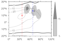
(a) AP_N1 (150 hPa)

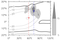
(b) AP_N2 (175 hPa)

Figure 11: Shift in location of $U_{max}$ in response to locations of heating. Zonal wind ( m s^-1) profile at pressure level where maximum zonal wind is attained. Precipitation contours ( mm day^-1) are shaded, ‘cross-diamond’ indicates location of $U_{max}$, ‘star’ is location of $P_{c}$. Aqua-planet with multiple off-equatorial heat sources in regions B, C and D shown in Fig. 9.

5.2.2 Importance of near-equatorial heating

Referring to Fig. 6c one can see that in the Ctrl simulation, during July, there is a broad precipitation zone just south of the Equator between 50^∘E-100^∘E and a zone just north of this zonal tongue centered at 60^∘E. Our goal is to induce similar precipitation patterns by imposing SST peaks in this region. Two such simulations have been conducted which are labelled as AP_E1 and AP_E2. The details are given in Tables 2, 3 and Fig. 9. Heating is present only in region E. Whenever there is an overlap, the maximum temperature is used which ensures that there are no kinks in the SST profiles. However the background SST is now 22^∘C. The rationale for this choice will be explained in the next subsection where multiple-heat source simulations are discussed. Both rectangular and circular SST profiles have been imposed. The peak SSTs do not exceed 29^∘C and are made to increase linearly to the peak value.

(a) AP_E2: Meridional section

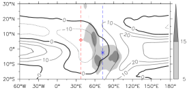
(b) AP_E2: Horizontal section: (225 hPa)

Figure 12: Zonal wind ( m s^-1) profile. LABEL:sub@E2-yz meridional section is at the longitude where $U_{max}$ is attained; LABEL:sub@NE2-xy horizontal cross-section at pressure level where $U_{max}$ is attained, ‘cross-diamond’ is location of $U_{max}$, ‘star’ is location of $P_{c}$, precipitation contours ( mm day^-1) are shaded: Aqua-planet with multiple heat sources in region E shown in Fig. 9.

From Table 3 it can be seen that the zonal wind speeds barely qualify as a jet. The speeds are hardly more than one-and-a-half times the easterly obtained for a uniform background simulation. The zonal wind structure is shown in Fig. 12. The location of peak zonal wind is at a lower height (below 200 hPa). The most important observation is the stark contrast in the meridional structure vis-a-vis the off-equatorial heating. From the meridional section (Fig. 12a), it is seen that the equator to pole tilt is towards higher pressure levels as in Ctrl and reanalysis. A low-level westerly of comparable strength extending below 500 hPa was also observed. Thus with just equatorial heating similar to real-planet, the vertical structure becomes baroclinic. Compared to reanalysis and real-planet there is a significant westerly to the east of the upper-level easterly. This signifies the reduced zonal extent of the easterly flows in comparison to single heat-source cases.

But the horizontal structure (Fig. 12b) immediately shows that the zonal wind structure is actually nowhere near the real-planet TEJ. The peak zonal wind was observed to be to the west of 90^∘W and hence very far from $P_{c}$. This far-off value has not been tabulated since the region chosen for locating the peak zonal wind is 0-90^∘E. In spite of the maximum heating being in the south of the equator, the easterly is in the northern hemisphere. All these show that near-equatorial heating is necessary for imparting a baroclinic structure somewhat resembling reality. But stand-alone near-equatorial heating is by itself insufficient to generate a jet structure that resembles the TEJ.

(a) AP_NE1: Meridional section

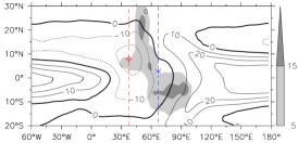
(b) AP_NE1: Horizontal section: (175 hPa)

(c) AP_NE2: Meridional section

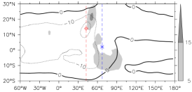
(d) AP_NE2: Horizontal section: (150 hPa)

Figure 13: Zonal wind ( m s^-1) profile. LABEL:sub@NE2-yz,LABEL:sub@NE3-yz meridional sections are at the longitude where $U_{max}$ is attained; LABEL:sub@NE2-xy,LABEL:sub@NE3-xy horizontal cross-section at pressure level where $U_{max}$ is attained, ‘cross-diamond’ is location of $U_{max}$, ‘star’ is location of $P_{c}$; precipitation contours ( mm day^-1) are shaded: Aqua-planet with multiple heat sources in regions B and E shown in Fig. 9.

5.2.3 Interplay between heating in near-Equator and Saudi Arabian regions

It is interesting to study the effect of heating in region B in addition to region E discussed above. These are the AP_NE1 and AP_NE2 simulations. It can be seen from Tables 1 and 3, that in these simulations the location of $U_{max}$ is closer to Ctrl simulation.

The meridional structure (Fig. 13a) is similar to the equatorial heating case. There is also the equator to pole tilt that is observed in real-planet and real-planet cases. The meridional structures show the familiar equator to pole tilt (as in reanalysis) till the precipitation in region B (Saudi Arabia) does not increase beyond a threshold. This increase can be inferred from Fig. 13c. Even then the depth is moderated by the equatorial heating effects. The change in tilt is due to precipitation being more in region B as can be seen from Fig. 13d in comparison to Fig. 13b. Here the equatorial heating in the latter is quite low and yet heating in B is not enough to increase the tilt in comparison to similar heating rates in the single heat source at 20^∘N).

This shows that heating near the equator is essential in creating a meridional structure resembling reanalysis and real-planet.

5.2.4 Effect of all heat sources except Pacific ocean warm pool region

The discussion on the influence of and near-equatorial and off-equatorial heating can now be used to combine all of them and study how close the net effect is on the Ctrl simulation. These are the AP_M1 to AP_M5 simulations (refer Table 3). In this effort, once again the role of the easternmost heating on the jet structure and location is studied. The only difference between AP_M1 and AP_M2, and AP_M3 to AP_M5 simulations is the presence of heating in region B in the latter set. Heating in region D is expected to have minimal role to play as it is not the easternmost source.

The first and foremost difference, as observed from Table 3, is in the zonal location of $U_{max}$. Precipitation in region B, as expected, causes a 15^∘-20^∘ westward shift in the jet location while the location of $P_{c}$ is hardly changed. This is clearly seen from Fig. 8 where points G and H are for AP_M1 and AP_M5 simulations. The zonal separation without heating in region B in the former causes the location of $U_{max}$ to be much closer to $P_{c}$. The jet zonal velocities are generally greater and this is because of heating in regions B,C and D (see section 5.2.3).

In all cases, the other zonal wind structures are similar in all cases (except for the difference in location of $U_{max}$ when heating in region B is present). Hence in Fig. 14 only AP_M5 simulation is shown. The upper-level meridional structure of the jet (Fig. 14a) resembles real-planet simulations (Fig. 3, left panel). The equator to pole tilt is always towards higher pressure levels. This demonstrates that in aqua-planet configuration, precipitation patterns similar to real-planet simulations result in meridional shapes similar to full AGCM simulations. The zonal jet lengths are still less than real-planet simulations.The eastward extent of the upper-level westerly intrusion is also unrealistic. This discrepancy will be addressed in section 5.2.5 below.

The relatively weaker and more westward location of peak zonal wind speed in AP_M3 simulation compared to AP_M5 is because the precipitation in region B in AP_M3 was much lower in comparison to AP_M5 (not shown). This once again underscores the influence of heating in region B (Saudi Arabia) in distorting the location of the jet in the Ctrl simulation. In spite of lower heating in region B in AP_M3 simulation, the meridional structure has the familiar equator to pole tilt (not shown). Except for the westerly to the east of 90^∘E, the overall TEJ simulated has a structure similar to Ctrl (Figs. 2b and 3c,LABEL:sub@cc-zx).

The location of the geopotential high (Fig. 14d) is now bears resemblance to Ctrl simulation (Fig. 4b). Although this peak in AP_M5 is shifted more eastwards in comparison, from Tables 1 and 3 it is seen that the location of $U_{max}$ as well as $P_{c}$ is also westwards in comparison. On closer inspection, from Fig. 8 (points J and H) it can be observed that the zonal and meridional separation between $P_{c}$ and $U_{max}$ almost the same. Thus in the aqua-planet simulations if all the SST profiles had been shifted westwards by $\sim$10^∘, then the mosaic of precipitation, zonal wind and geopotential heights would have shifted westwards by about the same amount. Then there would be more similarity with real-planet simulations.

It is also interesting to observe that the jet velocities increase by only $\sim$5 m s^-1 when compared with simulations with just an additional source at region B. In the previous single heat source simulations, the jet velocities increased when the intensity of heating increased both spatially and magnitude wise. Here, additional the heat source at 20^∘N does not significantly increase the jet strength. This shows that when multiple, well-distributed heat sources resembling reality are present, it is the intensity of heating and not the number of heating zones that determines the zonal wind strength.

(a) Meridional section

(b) Zonal section

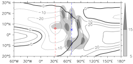
(c) Horizontal section (150 hPa)

(d) Velocity vectors and geopotential height (150 hPa)

Figure 14: Zonal wind ( m s^-1) profile. Vertical sections are at the LABEL:sub@M5-yz longitude and LABEL:sub@M5-yz latitude where $U_{max}$ is attained; LABEL:sub@M5-xy horizontal cross-section at pressure level where $U_{max}$ is attained, ‘cross-diamond’ is location of peak zonal wind, ‘star’ is location of $P_{c}$, precipitation contours ( mm day^-1) are shaded; LABEL:sub@M5-z3-xy velocity vectors and geopotential height ($\times 10^{3}$m) at 150 hPa, ‘cross-diamond’ is location of peak geopotential height, contour value is 13.79 which is 99.5% of peak. AP_M5 (Aqua-planet with multiple heat sources in regions B, C, D and E shown in Fig. 9).

5.2.5 Importance of heating in the Pacific Ocean warm pool

In all the above multiple heat source simulations, the greatest mismatch in zonal wind structure with the real-planet simulations is the westerly that was always present to the west of 90^∘E. This westerly was prominently reflected in all the zonal cross-sections. From Fig. 6 it is observed that in reanalysis there is significant precipitation occurring east of 100^∘E. Although in this region, in both Ctrl and noGlOrog, the precipitation is less than observation, there was significant precipitation in excess of 5 mm day^-1 in the Pacific warm pool which had not been incorporated in the aqua-planet configurations. Hence an additionale experiment, AP_M6, incorporating additional heating in region P as shown in Fig. 9, was conducted. The ratio of mean precipitation between 110^∘E-180^∘ and 20^∘S-30^∘N for AP_M6 and Ctrl is $\sim$0.95. Everywhere else the maximum SSTs were same as AP_M5. The results are shown in Fig. 15. The horizontal section (Fig. 15b) now shows the extension of the easterly beyond 90^∘E and this is also reflected in the zonal section (Fig. 15a). Thus the acceleration length of the TEJ is now closer to real-planet and reanalysis. The meridional section is similar to AP_M5 simulation and hence is not shown. The location and magnitudes of peak zonal wind in AP_M5 and AP_M6 are almost the same. Thus heating in the Pacific warm pool is necessary for the eastward extent of the TEJ.

(a) Zonal cross-section

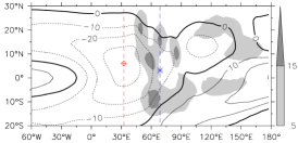
(b) Horizontal cross-section (150 hPa)

Figure 15: Zonal wind ( m s^-1) profile. LABEL:sub@M6-zx zonal wind at the latitude where $U_{max}$ is attained, LABEL:sub@M6-xy horizontal cross-section at pressure level where $U_{max}$ is attained, ‘cross-diamond’ is location of $U_{max}$, ‘star’ is location of $P_{c}$, precipitation contours ( mm day^-1) are shaded. AP_M6 (Aquaplanet with multiple heat sources in all regions, except S, shown in Fig. 9).

6 Conclusions

The July climatological structure of the Tropical Easterly Jet in observations has been studied and compared with the simulations by an AGCM. The TEJ in reanalysis in July 1998 and 2002 had significant zonal shifts. Reduced precipitation in the Indian region in 2002 made the jet have its maxima in the southern Indian peninsula as compared to 1988 when high rainfall in the Indian region resulted in the TEJ having its maxima over the Arabian sea region.

The TEJ in the Ctrl simulation has errors in the spatial location; otherwise the simulated TEJ bears similarities with observations. Removing orography left the spatial location and structure is practically unchanged. This leads us to conclude that the TEJ is not directly influenced by orography. The primary reason for the shift in the simulated TEJ was because the location of precipitation in both Ctrl and noGlOrog is westwards when compared to reanalysis.

Additional experiments were conducted to check if the TEJ is primarily influenced by latent heating. Changing the deep-convective relaxation time scale both in Ctrl and noGlOrog simulations confirmed this. In these new simulations the precipitation is more accurately simulated and most importantly anomalous precipitation in Saudi Arabia no longer occurred. The jet followed the shift in precipitation and relocated to the correct climatological position. The absence of orography once again had no impact on the location of the jet. This conclusively proves that the TEJ is independent of orography. Changing the default value of deep convective time-scale also demonstrated the secondary role of orography. Both Ctrl$\tau_{d12}$ and noGlOrog$\tau_{d12}$ have very similar precipitation patterns and hence the TEJ in both is correctly simulated.

To understand why the TEJ was shifted westward in the AGCM, aqua-planet experiments were conducted.

1. The simulation of TEJ in an aqua-planet configuration of the AGCM shows that orography and land-sea interactions are not as important as latent heat release.

2. The total acceleration length is cirrelated to the zonal extent of the heating.

3. A heat source at 20^∘N appears more to be robust in generating wind speeds that may be referred to as a jet while equatorial heating alone does not generate TEJ.

4. Equatorial heating is necessary to generate a strong low-level westerly that imparts the vertical baroclinic structure to the TEJ. However it is insufficient in generating true TEJ horizontal structure.

5. Equatorial heating is essential to create meridional structures seen in observations and full AGCM simulations. Greater poleward depth is possible only if equatorial heating is present.

6. The longitudinal location of peak zonal wind is influenced by the off-equatorial heating that is closest to it. It has been demonstrated that rainfall in Saudi Arabia causes the extreme westward shift of the TEJ in full AGCM simulations in comparison to observations.

7. Heating in the Pacific warm pool is essential to cause eastward extension and increased acceleration length of the TEJ.

When all the important heat sources are incorporated in the aqua-planet configuration, many observed features of the TEJ were simulated. Thus aqua-planet simulations play an important role in understanding the role of heat sources in the absence of any influence of land and orography.

References

- Adler et al. (2003) R. F. Adler, G. J. Huffman, A. Chang, R. Ferraro, P.-P. Xie, J. Janowiak, B. Rudolf, U. Schneider, S. Curtis, D. Bolvin, A. Gruber, J. Susskind, P. Arkin, and E. Nelkin. The version-2 Global Precipitation Climatology Project (GPCP) monthly precipitation analysis (1979-present). Journal of Hydrometeorology, 4:1147–1167, 2003.
- Bhat (2006) G. S. Bhat. The Indian drought of 2002 – a sub-seasonal phenomenon? Quarterly Journal of the Royal Meteorological Society, 132(621):2853–2602, 2006. doi: 10.1256/qj.05.13.
- Bordoni and Schneider (2008) S. Bordoni and T. Schneider. Monsoons as eddy-mediated regime transitions of the tropical overturning circulation. Nature Geosciences, 1(8):515–519, 2008. doi: 10.1038/ngeo248.
- Briegleb (1992) B. P. Briegleb. Delta-Eddington approximation for solar radiation in the NCAR Community Climate Model. Journal of Geophysical Research, 97(D7):7603–7612, 1992. doi: 10.1029/92JD00291.
- Camberlin (1995) P. Camberlin. June-september rainfall in north-eastern Africa and atmospheric signals over the tropics. International Journal of Climatology, 15(7):773–783, 1995. doi: 10.1002/joc.3370150705.
- Chakraborty et al. (2008) A. Chakraborty, R. S. Nanjundiah, and J. Srinivasan. Impact of African orography and the Indian summer monsoon on the low-level Somali jet. International Journal of Climatology, 29(7):983–992, 2008.
- Chen and van Loon (1987) T.-C. Chen and H. van Loon. Interannual variation of the Tropical Easterly Jet. Monthly Weather Review, 115:1739–1759, 1987. doi: 10.1175/1520-0493(1987)115¡1739:IVOTTE¿2.0.CO;2.
- Davis et al. (2012) R. N. Davis, Y.-W. Chen, S. Miyahara, and N. J. Mitchell. The climatology, propagation and excitation of ultra-fast Kelvin waves as observed by meteor radar, Aura MLS, TRMM and in the Kyushu-GCM. Atmos. Chem. Phys., 12:1865–1879, 2012. doi: 10.5194/acp-12-1865-2012.
- Flohn (1965) H. Flohn. Thermal effects of the Tibetan Plateau during the Asian monsoon season. Correspondence, University of Bonn, 1965.
- Flohn (1968) H. Flohn. Contributions to a meteorology of the Tibetan highland. Atmospheric Science Paper 130, Colorado State University, Colorado State University, Fort Collins, 1968.
- Gill (1980) A. E. Gill. Some simple solutions for heat-induced tropical circulation. Quarterly Journal of the Royal Meteorological Society, 106(449):447–462, 1980.
- Hack (1994) J. J. Hack. Parameterization of moist convection in the National Center for Atmospheric Research Community Climate Model (CCM2). Journal of Geophysical Research, 99(D3):5551–5568, 1994. doi: 10.1029/93JD03478.
- Hoskins and Rodwell (1995) B. J. Hoskins and M. J. Rodwell. A model of the Asian summer monsoon. Part 1: The global scale. Journal of the Atmospheric Sciences, 52:1329–1340, 1995. doi: 10.1175/1520-0469(1995)052¡1329:AMOTAS¿2.0.CO;2.
- Hulme and Tosdevin (1989) M. Hulme and N. Tosdevin. The Tropical Easterly Jet and Sudan rainfall: A review. Theoretical and Applied Climatology, 39(4):179–187, 1989. doi: 10.1007/BF00867945.
- Hurrell et al. (2006) J. W. Hurrell, J. J. Hack, A. S. Phillips, J. Caron, and J. Yin. The dynamical simulation of the Community Atmosphere Model version 3 (CAM3). Journal of Climate, 19:2162–2183, 2006. doi: 10.1175/JCLI3762.1.
- Jingxi and Yihui (1989) L. Jingxi and D. Yihui. Climatic study on the summer Tropical Easterly Jet at 200 hPa. Advances in Atmospheric Sciences, 6(2):215–226, 1989. doi: 10.1007/BF02658017.
- Kalnay et al. (1996) E. Kalnay, M. Kanamitsu, R. Kistler, W. Collins, D. Deaven, L. Gandin, M. Iredell, S. Saha, G. White, J. Woollen, Y. Zhu, M. Chelliah, W. Ebisuzaki, W. Higgins, J. Janowiak, K. C. Mo, C. Ropelewski, J. Wang, A. Leetma, R. Reynolds, R. Jenne, and D. Joseph. The NCEP/NCAR 40-year reanalysis project. Bulletin of the American Meteorological Society, 77:437–471, 1996. doi: 10.1175/1520-0477(1996)077¡0437:TNYRP¿2.0.CO;2.
- Koteswaram (1958) P. Koteswaram. The easterly jet stream in the tropics. Tellus, 10(1):43–57, 1958. doi: DOI: 10.1111/j.2153-3490.1958.tb01984.x.
- Krishnamurti (1971) T. N. Krishnamurti. Observational study of the tropical upper tropospheric motion field during the northern hemisphere summer. Journal of Applied Meteorology, 10:1066–1096, 1971.
- Kucharski et al. (2009) F. Kucharski, A. Bracco, J. H. Yoo, A. M. Tompkins, L. Feudale, P. Rutic, and Dell’ Aquila. A Gill-Matsuno-type mechanism explains the tropical Atlantic influence on African and Indian monsoon rainfall. Quarterly Journal of the Royal Meteorological Society, 135(640):569–579, 2009. doi: 10.1002/qj.406.
- Lee (1999) S. Lee. Why are the climatological zonal winds easterly in the equatorial upper troposphere? Journal of the Atmospheric Sciences, 56:1353–1363, 1999.
- Liu et al. (2007) Y. Liu, B. J. Hoskins, and M. Blackburn. Impact of Tibetan orography and heating on the summer flow over Asia. Journal of the Meteorological Society of Japan, 85B:1–19, 2007. doi: 10.2151/jmsj.85B.1.
- Mishra (1987) S. K. Mishra. Linear barotropic instability of the Tropical Easterly Jet on a sphere. Journal of the Atmospheric Sciences, 44(2):373–383, 1987.
- Mishra (1993) S. K. Mishra. Nonlinear barotropic instability of the upper-tropospheric Tropical Easterly Jet on the sphere. Journal of the Atmospheric Sciences, 50(21):3541–3552, 1993.
- Neale and Hoskins (2001) R. B. Neale and B. J. Hoskins. A standard test for AGCMs including their physical parametrizations. II: Results for The Met Office Model. 1, 2001. doi: 10.1006/asle.2000.0020.
- Nicholson et al. (2007) S. E. Nicholson, A. I. Barcilon, M. Challa, and J. Baum. Wave activity on the Tropical Easterly Jet. Journal of the Atmospheric Sciences, 64:2756–2763, 2007. doi: 10.1175/JAS3946.1.
- Raghavan (1973) K. Raghavan. Tibetan anticyclone and Tropical Easterly Jet. Pure and Appied Geophysics, 110(1):2130–2142, 1973. doi: 10.1007/BF00876576.
- Rajendran et al. (2013) K. Rajendran, A. Kitoh, and J. Srinivasan. Effect of SST variation on ITCZ in APE simulations. Journal of the Meteorological Society of Japan, 91A:195–215, 2013.
- Ramanathan and Downey (1986) V. Ramanathan and P. Downey. A nonisothermal emissivity and absorptivity formulation for water vapor. Journal of Geophysical Research, 91:8649–8666, 1986. doi: 10.1029/JD091iD08p08649.
- Rasch and Kristjánsson (1998) P. J. Rasch and J. E. Kristjánsson. A comparison of the CCM3 model climate using diagnosed and predicted condensate parameterizations. Journal of Climate, 11:1587–1614, 1998. doi: 10.1175/1520-0442(1998)011¡1587:ACOTCM¿2.0.CO;2.
- Rayner et al. (2003) N. A. Rayner, D. E. Parker, E. B. Horton, C. K. Folland, L. V. Alexander, and D. P. Rowell. Global analyses of sea surface temperature, sea ice and night marine air temperature since the late nineteenth century. Journal of Geophysical Research, 108(D14):4407, 2003. doi: 10.1029/2002JD002670.
- Reynolds et al. (2002) R. W. Reynolds, N. A. Rayner, T. M. Smith, D. C. Stokes, and W. Wang. An improved in situ and satellite SST analysis for climate. Journal of Climate, 15:1609–1625, 2002. doi: 10.1175/1520-0442(2002)015¡1609:AIISAS¿2.0.CO;2.
- Sathiyamoorthy (2005) V. Sathiyamoorthy. Large scale reduction in the size of the Tropical Easterly Jet. Geophysical Research Letters, 32(14):1–4, 2005. doi: 10.1029/2005GL022956.
- Sathiyamoorthy et al. (2007) V. Sathiyamoorthy, P. K. Pal, and P. C. Joshi. Intraseasonal variability of the Tropical Easterly Jet. Meteorology and Atmospheric Physics, 96(3-4):305–316, 2007. doi: 10.1007/s00703-006-0214-7.
- Schneider (2006) T. Schneider. The general circulation of the atmosphere. Annu. Rev. Earth Planet. Sci., 34:655–688, 2006.
- Sikka (2003) D. R. Sikka. Evaluation of monitoring and forecasting of summer monsoon over India and a review of monsoon drought of 2002. Proceedings of the Indian National Science Academy, 69, A(5):479–504, 2003.
- Slingo (1989) A. Slingo. A GCM parameterization for the shortwave radiative properties of clouds. Journal of the Atmospheric Sciences, 46:1419–1427, 1989. doi: 10.1175/1520-0469(1989)046¡1419:AGPFTS¿2.0.CO;2.
- Uppala et al. (2005) S. M. Uppala, P. W. Kallberg, A. J. Simmons, U. Andrae, V. D. Bechtold, M. Fiorino, J. K. Gibson, J. Haseler, A. Hernandez, G. A. Kelly, X. Li, K. Onogi, S. Saarinen, N. Sokka, R. P. Allan, E. Andersson, K. Arpe, M. A Balmaseda, A. C. M. Beljaars, L. Van De Berg, J. Bidlot, N. Bormann, S. Caires, F. Chevallier, A. Dethof, M. Dragosavac, M. Fisher, M. Fuentes, S. Hagemann, E. Holm, B. J. Hoskins, L. Isaksen, P. A. E. M Janssen, R. Jenne, A. P. McNally, J. F. Mahfouf, J. J. Morcrette, N. A. Rayner, R. W. Saunders, P. Simon, A. Sterl, K. E. Trenberth, A. Untch, D. Vasiljevic, P. Viterbo, and J. Woollen. The ERA-40 Re-analysis. Quarterly Journal of the Royal Meteorological Society, 131(612):2961–3012, 2005. doi: 10.1256/qj.04.176.
- Wang (2006) B. Wang. The Asian Monsoon. Springer, 2006.
- Xie and Arkin (1997) P. Xie and P. A. Arkin. Global precipitation: A 17-year monthly analysis based on gauge observations, satellite estimates, and numerical model outputs. Bulletin of the American Meteorological Society, 78(11):2539–2558, 1997. doi: 10.1175/1520-0477(1997)078¡2539:GPAYMA¿2.0.CO;2.
- Ye (1981) D. Ye. Some characteristics of the summer circulation over the Qighai-Xizang (Tibet) Plateau and its neighborhood. Bulletin of the American Meteorological Society, 62:14–19, 1981. doi: 10.1175/1520-0477(1981)062¡0014:SCOTSC¿2.0.CO;2.
- Zhang and McFarlane (1995) G. J. Zhang and N. A. McFarlane. Sensitivity of climate simulations to the parameterization of cumulus convection in the Canadian Climate Centre general circulation model. Atmosphere-Ocean, 33(3):407–446, 1995. doi: 10.1080/07055900.1995.9649539.
- Zhang et al. (2003) M. Zhang, C. S. Bretherton, J. J. Hack, and P. J. Rasch. A modified formulation of fractional stratiform condensation rate in the NCAR Community Atmospheric Model CAM2. Journal of Geophysical Research, 108(D1), 2003. doi: 10.1029/2002JD002523.
- Zhang et al. (2002) Q. Zhang, G. Wu, and Y. Qian. The bimodality of the 100 hPa south asia high and its relationship to the climate anomaly over east asia in summer. Journal of the Meteorological Society of Japan, 80(4):733–744, 2002. doi: 10.2151/jmsj.80.733.