Abstract

A calculation by Jacobson [1] strongly implies that the field equations which describe gravity are emergent phenomena. In this paper, the method is extended to the case of a non-commutative spacetime. By making use of a non-commutative version of the Raychaudhuri equation, a new set of non-commutative Einstein equations is derived. The results demonstrate that it is possible to use spacetime thermodynamics to work with non-commutative gravity without the need to vary a non-commutative action.

1 Introduction

In four dimensions, black hole solutions to the Einstein equations are determined solely by mass, electric charge and angular momentum [2]. In hindsight, this provides the first small hint that the behaviour of black holes is in some way similar to that of classical thermodynamics. When describing a classical gas, it is not feasible to keep an exhaustive list of all positions and velocities of all the gas particles. We can restrict ourselves to a few variables and still compute meaningful physical quantities. Similarly, a star can be described by many physical variables, but after its collapse we are forced into using only three.

This similarity is, of course, nothing more than a hint. Only with the identification of the area of a black hole with entropy and the establishment of the four laws of black hole mechanics [2][3], did black hole thermodynamics become something which could be meaningfully explored and questioned. This means, however, that an entirely valid question would be to ask whether the analagous behaviour signifies something deeper.

The evidence for spacetime as a thermodynamic system grew when, in 1995, Jacobson [1] brought the idea of black hole thermodynamics full circle by showing that the Einstein equations can be derived as an equation of state. The assumption that needs to be made is that entropy and the area of causal horizons are still equal, up to some multiplicative constant. This is not an unreasonable assumption since entropy measures information and causal horizons hide information from observers in space time.

The Einstein equations stipulate how the geodesics of spacetime bend in response to the presence of matter. However, these field equations need not be assumed from the outset. Simply insist that for some matter crossing a causal horizon, $\delta Q=TdS$ holds $(\delta Q$ being the amount of energy moving across the horizon, $T$ being the Unruh temperature and $dS$ being the associated increase in entropy of the universe on the other side of the causal horizon). From the only initial assumption, $\delta Q=TdS=\eta dA$ since $dS=\eta dA$. What this demonstrates is that you only need assume the entropy-area relation to show that matter will bend the geodesics in a spacetime. It will be shown below that these simple arguments will lead to the Einstein equations. This is a thermodynamic derivation of the equations of General Relativity and it shows that they are, in fact, an equation of state.

If the Einstein equations truly are an equation of state, this begs the question of whether or not other equations of state exist. While it is possible to arrive at other equations of state by changing the entropy functional $\delta S=\kappa\delta A$, this is not the approach which will be followed in this paper. Rather, the reasoning will be analogous to that of classical thermodynamics. Instead of making assumptions about the thermodynamic functionals, instead we change the assumptions about the physics of the system in question.

An example of this is seen in moving from the ideal gas equation

$$PV=nRT$$ (1)

to the Van der Waals equation

$$\left(P+\frac{n^{2}a}{V^{2}}\right)\left(V-nb\right)=nRT.$$ (2)

The ideal gas law does not allow for a system of gas particles to interact, nor for the particles to have any size. By giving the particles size and the ability to interact, no broad statement about thermodynamics is made. All that is made is a change in the assumptions about the microstructure of the thermodynamical system. Additionally, no information about the kinetic theory of gases nor their statistical mechanics was needed to derive the Van der Waals equation. This surprising paucity of information shows that it might be possible to derive a new spacetime equation of state with relatively simple assumptions about spacetime microstructure.

An assumption that is tempting to make is that there is a minimum length in spacetime. To see a simple reason why, recall that entropy can be written as

$$S=k\ln\Omega$$ (3)

where $\Omega$ is the number of states accessible to the system. Since $\Omega$ is an integer, the value of $S$ cannot be continuous - it can only take on certain values. Note, however, that in classical geometry the area of a black hole is continuous and therefore the entropy given by $S=\nicefrac{{A}}{{4}}$ is also continuous. This seems like a contradiction but we do similar work in statistical mechanics. We treat variables semiclassically and use them as if they were continuous, but we know from the microscopic nature of the theory that they are in fact quantized.

The above might be a simple argument but it is nonetheless forceful and reason enough to look for different field equations of spacetime in which area quantization is enforced from the beginning. In this paper we will attempt to enforce the area quantization by requiring that the spacetime coordinates obey the non-commutative relation $\left[x^{i},x^{j}\right]=i\theta^{ij}$. Once non-commutativity is imposed, the work of Jacobson will be used to show how a non-commutative version of the Einstein Field Equations can be derived.

In section 2, Jacobson’s argument is reviewed. Section 3 begins by addressing concerns over imposing non-commutativity on spacetime and then provides information on the mathematics needed to work with functions on a non-commutative manifold. After this, a non-commutative version of the Raychaudhuri equation is derived and used to repeat Jacobson’s method for the case of non-commutative manifold.

2 Review of Jacobson’s argument

Let us briefly recapitulate the argument of [1]. Assume that there is some accelerating observer in a spacetime, the field equations of which are not specified at the beginning. Since the observer has a causal horizon and there are not yet any field equations, we are free to specify how the generators of the horizon behave when matter crosses them. If we assume that the area of the horizon changes proportionally to the entropy of any matter crossing the horizon, the Raychaudhuri equation can be used to calculate the change in area of the horizon. If this done, we are shown in [1] that the Einstein equations come out as a result.

To see how the Einstein equations can be interpreted as an equation of state, pick a point $p$ in spacetime and make the approximation that the space around $p$ is, locally, Minkowskian. Now choose a small patch of 2-surface which contains $p$ and call this patch $O$.

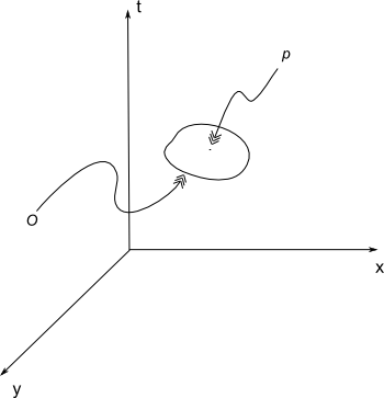
Figure 1: Minkowski space containing $O$ and $p.$

Choose one side of the boundary as the past of $O.$

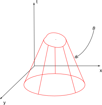
Figure 2: The boundary $B$ of the past of the patch $O.$

Close to the point $p,$ this boundary is a congruence of null geodesics orthogonal to $O$. This congruence constitutes the causal horizon which will be studied in the derivation.

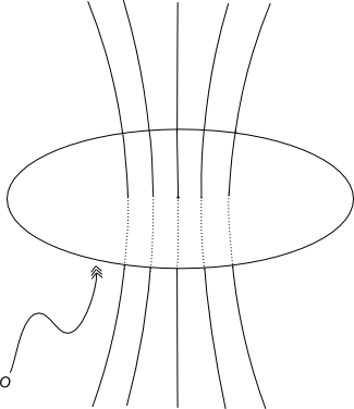
Figure 3: The null geodesics orthogonal to $O$. We can use the Raychaudhuri equation to study these geodesics and hence the behaviour of the the patch $O.$

Choose the patch so that the expansion and shear of the congruence vanish close to $p$. It is always possible to do this. Note that the rotation vanishes due to the fact that the congruence is normal to the 2-surface patch. By making this construction, a local Rindler horizon has been defined around $p$. There are local Rindler horizons in all null directions around a spacetime point due to the fact an observer can accelerate in any direction.

Since an approximately flat region of spacetime exists near our point $p$ and around the patch $O$, the spacetime there will have all the usual Poincare symmetries. This makes it possible to find an approximate Killing field $\chi^{a}$ generating Lorentz boosts which are orthogonal to $O$ and which vanish at $O.$ Suppose now that some stress energy tensor $T_{ab}$ is defined in the spacetime. The flow of energy orthogonal to the patch $O$ will be given by $T_{ab}\chi^{a}$.

Now choose $\chi^{a}$ to be future pointing to the inside past of our patch $O$. The energy flux to the past of the patch will then be

$$\delta Q=\int_{H}T_{ab}\chi^{a}d\Sigma^{b}$$ (4)

where the integral is over the generators of the inside past horizon of $O$.

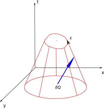
Figure 4: The heat flux across the boundary $B.$ This picture illustrates that heat (in whatever form) is moving across the causal horizon $B$ into an area of spacetime from which a null ray can reach the Rindler observer.

Call the tangent vector to the horizon generators $k^{a}$ and let $\lambda$ be the affine parameter which vanishes at the patch $O$ and is negative to the past of $O.$ This implies

$$\chi^{a}=-\kappa\lambda k^{a}$$ (5)

and that the small patch of directed surface area is

$$d\Sigma^{a}=k^{a}d\lambda dA$$ (6)

where the $dA$ is an infinitesimal piece of horizon. Rename the energy flux to heat flux, as can be done in ordinary thermodynamics, and write it as:

$$\delta Q=-\kappa\int_{H}\lambda T_{ab}k^{a}k^{b}d\lambda dA$$ (7)

Making use of the entropy-area rule from black hole thermodynamics makes it possible to say that the entropy of this heat flux is associated with a small change in the area of the horizon:

$$dS=\eta dA.$$ (8)

It is best to leave the constant of proportionality undetermined for now - the rest of the derivation is insensitive to this. A small patch of cross-sectional area of the null horizon generators is given by:

$$\delta A=\int_{H}\theta d\lambda dA.$$ (9)

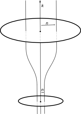
Figure 5: The horizon generators expand as the entropy moves across the horizon.

Recall that the thermodynamic relations being used are:

$$\delta Q=TdS=\eta\delta A.$$ (10)

Use the Unruh temperature as the temperature in the above, then set

$$-\kappa\int_{H}\lambda T_{ab}k^{a}k^{b}d\lambda dA=\int_{H}\theta d\lambda dA$$ (11)

and employ the Raychaudhuri equation for null surfaces. Recall that the congruence has been chosen to give vanishing expansion and shear, so that the Raychaudhuri equation reduces to

$$\frac{d\theta}{d\lambda}=-R_{ab}k^{a}k^{b}$$ (12)

and upon integration, $\theta$ integrates to $-\lambda R_{ab}k^{a}k^{b}.$ This tells us that (11) becomes

$$-\kappa\int_{H}\lambda T_{ab}k^{a}k^{b}d\lambda dA=\int_{H}-\lambda R_{ab}k^{a}k^{b}d\lambda dA$$ (13)

and we get to

$$T_{ab}k^{a}k^{b}=\left(\frac{\hbar\eta}{2\pi}\right)R_{ab}k^{a}k^{b}$$ (14)

for all null $k^{a}.$ Given $g_{ab}k^{a}k^{b}=0$ for null $k^{a},$ the metric tensor can be added into (14) for free

$$T_{ab}k^{a}k^{b}=\left(\frac{\hbar\eta}{2\pi}\right)R_{ab}k^{a}k^{b}+fg_{ab}k^{a}k^{b}$$ (15)

Where $f$ is some undetermined function. Since the expressions above are true for $any$ null vector, the result is:

$$T_{ab}=\left(\frac{\hbar\eta}{2\pi}\right)R_{ab}+fg_{ab}.$$ (16)

Making use of the fact that $T_{ab}$ is divergence-free and the contracted Bianchi identity to specify $f=-\frac{1}{2}R+\Lambda$, where $\Lambda$ is a constant, this gives [1]:

$$\left(\frac{2\pi}{\hbar\eta}\right)T_{ab}=R_{ab}-\frac{1}{2}Rg_{ab}+\Lambda g_{ab}$$ (17)

Jacobson’s calculation brings spacetime thermodynamics full circle. By studying the behaviour of back holes, one can infer that the solutions to the Einstein equations encode the area-entropy relationship. By assuming that the entropy-area relationship exists, one can then get back to the Einstein equations. More importantly, by demonstrating that there exists a thermodynamic derivation of the equations of general relativity, the result demonstrates that the geometrical variables of gravity (and not just the black hole parameters) can be treated as thermodynamic variables.

3 The Einstein-Van der Waals Equation

Care must be taken when it comes to making assumptions about the microstructure of spacetime - simply placing spacetime on a lattice will break diffeomorphism invariance. A more subtle and perhaps more useful choice is to rather state that coordinates on spacetime do not commute:

$$\left[x^{i},x^{j}\right]=i\theta^{ij}.$$ (18)

This statement has a strong analogue in quantum mechanics. By thinking of phase space as a manifold, the quantum mechanical coordinates $\hat{x},\hat{p}$ on the phase space manifold obey the commutation relation

$$\left[\hat{x},\hat{p}\right]=i\hbar$$ (19)

which demonstrates that the geometry of the phase space manifold is, in fact, noncommutative. This setup is desirable because in both cases it gives us cells of a definite area, but does so without forcing either manifold onto a lattice.

What is desired is a way to implement these commutation relations which still allows us to perform calculations in a straightforward manner. The approach which will be followed in this paper is to replace the ordinary multiplication of functions with the Moyal star product multiplication. This star product represents the deformation of a classical, commutative theory (the algebra of smooth functions on the manifold) in the sense that it turns its commutative product into a non-commutative product.

3.1 Background

Several steps need to be taken before we can arrive at a new set of field equations. First, ordinary multiplication must be replaced the Moyal star product. This is an operation which has the desirable properties of associativity, bilinearity and the Leibniz rule. For scalars $a,b$:

$$(f\star g)\star h=f\star(g\star h)$$ (20)

$$af\star bg=abf\star g$$ (21)

$$\partial_{\mu}(f\star g)=(\partial_{\mu}f)\star g+f\star(\partial_{\mu}g).$$ (22)

In order to take advantage of the above, it will be best to use the tetrad formalism of general relativity. To set notation, we write:

$$g_{\mu\nu}e_{a}^{\mu}e_{b}^{\nu}=\eta_{ab}$$ (23)

$$g_{\mu\nu}=e_{\mu}^{a}e_{\nu}^{b}\eta_{ab}.$$ (24)

The Christoffel symbols and the spin connection are related by

$$\omega_{\mu}^{\;\;a}\;{}_{b}=e_{\nu}^{a}e_{b}^{\lambda}\Gamma_{\mu\lambda}^{\nu}-e_{b}^{\lambda}\partial_{\mu}e_{\lambda}^{a}.$$ (25)

The spin connection obeys its own transformation law

$$\omega_{\mu}^{\;\;a^{\prime}}\;{}_{b^{\prime}}=\Lambda^{a^{\prime}}\;_{a}\Lambda_{b^{\prime}}\;^{b}\omega_{\mu}^{\;\;a}\;{}_{b}-\Lambda_{b^{\prime}}\;^{c}\partial_{\mu}\Lambda^{a^{\prime}}\;_{c}.$$ (26)

which resembles the transformation law of the connection of a gauge-invariant theory:

$$A_{\mu}^{\;\;A^{\prime}}\;{}_{B^{\prime}}=O^{A^{\prime}}\;_{A}O_{B^{\prime}}^{\;B}A_{\mu}^{\;\;A}\;{}_{B}-O_{B^{\prime}}^{\;C}\partial_{\mu}O^{A^{\prime}}\;_{C}.$$ (27)

The last step in the mathematical setup is to make use of the Sieberg-Witten map [4]. This is a way to map between a gauge theory living on a commutative manifold and that same gauge theory living on a noncommutative manifold. For $R^{\mu}$ with coordinates $x^{i},$ impose coordinate noncommutativity by saying that the coordinates obey the algebra:

$$\left[x^{i},x^{j}\right]=i\theta^{ij}$$

where $\theta$ is real. We want to use this to deform the algebra of functions living on $R^{n}$ to a noncommutative algebra such that

$$f\star g=fg+i\frac{1}{2}\theta^{ij}\partial_{i}f\partial_{j}g+O(\theta^{2}).$$ (28)

The unique solution to this problem is [4]:

$$\begin{array}[t]{rl}f(x)\star g(x)&=exp\left[\frac{i}{2}\theta^{ij}\frac{\partial}{\partial\alpha^{i}}\frac{\partial}{\partial\beta^{j}}\right]f\left(x+\alpha\right)g\left.\left(x+\beta\right)\right|_{\alpha=\beta=0}\\ &=fg+i\frac{1}{2}\theta^{ij}\partial_{i}f\partial_{j}g+O(\theta^{2}).\end{array}$$ (29)

If the functions $f$ and $g$ are matrix-valued functions, then the star product becomes the tensor product of matrix multiplication with the star product of functions as just defined.

For a commutative gauge theory, the gauge transformations and field strength are written as

$$\delta_{\lambda}A_{i}=\partial_{i}+i\left[\lambda,A_{i}\right],$$ (30)

$$F_{ij}=\partial_{i}A_{j}-\partial_{j}A_{i}-i\left[A_{i},A_{j}\right]$$ (31)

and

$$\delta_{\lambda}F_{ij}=i\left[\lambda,F_{ij}\right].$$ (32)

For a non-commutative gauge theory, we apply the same formulae for the gauge transformation law and the field strength, except that the matrix multiplication is defined by the star product. If the gauge parameter is $\hat{\lambda}$ the gauge transformations and field strength of non-commutative Yang-Mills theory are:

$$\hat{\delta}_{\hat{\lambda}}\hat{A}_{i}=\partial_{i}\hat{\lambda}+i\hat{\lambda}\star\hat{A}_{i}-i\hat{A}_{i}\star\hat{\lambda}$$ (33)

$$\hat{F}_{ij}=\partial_{i}\hat{A}_{j}-\partial_{j}\hat{A}_{i}-i\hat{A}_{i}\star\hat{A}_{j}+i\hat{A}_{j}\star\hat{A}_{i}$$ (34)

$$\hat{\delta}_{\hat{\lambda}}\hat{F}_{ij}=i\hat{\lambda}\star\hat{F}_{ij}-i\hat{F}_{ij}\star\hat{\lambda}.$$ (35)

To first order in $\theta,$ these expressions are:

$$\hat{\delta}_{\hat{\lambda}}\hat{A}_{i}=\partial_{i}\hat{\lambda}-\theta^{kl}\partial_{k}\hat{\lambda}\partial_{l}\hat{A}_{i}+O(\theta^{2})$$ (36)

$$\hat{F}_{ij}=\partial_{i}\hat{A}_{j}-\partial_{j}\hat{A}_{i}-\theta^{kl}\partial_{k}\hat{A_{i}}\partial_{l}\hat{A}_{j}+O(\theta^{2})$$ (37)

$$\hat{\delta}_{\hat{\lambda}}\hat{F}_{ij}=-\theta^{kl}\partial_{k}\hat{\lambda}\partial_{l}\hat{F}_{ij}+O(\theta^{2}).$$ (38)

It now remains to find a mapping from ordinary gauge fields $A$ to non-commutative gauge fields $\hat{A}$ which are local to any finite order in $\theta.$ It is also necessary to impose the requirement that if two ordinary gauge fields $A$ and $A^{\prime}$ are equivalent by an ordinary gauge transformation $U=exp(i\lambda),$ then the noncommutative gauge fields $\hat{A}$ and $\hat{A^{\prime}}$ will be gauge equivalent by a non-commutative gauge transformation ${U=exp(i\hat{\lambda})}.$ Note that $\hat{\lambda}$ depends on $A$ and $\lambda.$

Take the gauge fields to be of rank $N$, so that the gauge parameters are $N\times N$ matrices. It is necessary to find a mapping between commutative and non-commutative fields such that

$$\hat{A}(A)+\hat{\delta}_{\hat{\lambda}}\hat{A}(A)=\hat{A}(A+\delta_{\lambda}A)$$ (39)

where the variables $\lambda$ and $\hat{\lambda}$ are infinitesimal. This ensures that if $A$ undergoes a transform by $\lambda,$ then the transformation of $\hat{A}$ by $\hat{\lambda}$ is equivalent. This forces ordinary fields which are gauge-equivalent to be mapped to non-commutative gauge fields which are also gauge-equivalent. Working to first order in $\theta$ and write $\hat{A=A+A^{\prime}(A)}$ and $\hat{\lambda}(\lambda,A)=\lambda+\lambda^{\prime}(\lambda,A).$ Thus, we expand (40) as

$$\begin{array}[t]{l}A^{\prime}_{i}(A+\delta_{\lambda}A)-A^{\prime}_{i}(A)-\partial_{i}\lambda^{\prime}-i\left[\lambda^{\prime},A_{i}\right]-i\left[\lambda,A^{\prime}_{i}\right]\\ =-\frac{1}{2}\theta^{kl}\left(\partial_{k}\lambda\partial_{l}A_{i}+\partial_{l}A_{i}\partial_{k}\lambda\right)+O(\theta^{2})\end{array}$$ (40)

where all the products appearing in the above are ordinary matrix products. Equation (19) is solved by

$$\hat{A}_{i}(A)=A_{i}+A^{\prime}_{i}(A)=A_{i}-\frac{1}{4}\theta^{kl}\left\{A_{k},\partial_{l}A_{i}+F_{li}\right\}+O(\theta^{2})$$ (41)

and

$$\hat{\lambda}_{i}(\lambda,A)=\lambda+\lambda^{\prime}_{i}(\lambda,A)=\lambda+\frac{1}{4}\theta^{ij}\left\{\partial_{i}\lambda,A_{j}\right\}+O(\theta^{2}).$$ (42)

The gauge strength is then written as

$$\hat{F}_{ij}=F_{ij}+\frac{1}{4}\theta^{kl}\left(2\left\{F_{ik},F_{jl}\right\}-\left\{A_{k},D_{l}F_{ij}+\partial_{l}F_{ij}\right\}\right)+O(\theta^{2}).$$ (43)

Equations (42), (43) and (44) illustrate what a gauge theory would look like if it were to live on a noncommutative manifold and they do so in terms of what the field looks like on a regular, commutative manifold. There now exists a new noncommutative theory expressed entirely in terms of expressions and functions we already know.

So far, the work has only been done to first order. To work to higher orders in $\theta,$ consider mapping the field $\hat{A}(\theta)$ to $\hat{A}(\theta+\delta\theta).$ The only property of the $\star-$product that one needs to check in order to see that (43) and (44) satisfy (40) is

$$\delta\theta^{ij}\frac{\partial}{\partial\theta^{ij}}(f\star g)=\frac{i}{2}\delta\theta^{ij}\frac{\partial f}{\partial x^{i}}\star\frac{\partial g}{\partial x^{j}}$$ (44)

when $\theta=0.$ Since this is true for any value of $\theta,$ it is possible to write down formulas which tell us how $\hat{A}(\theta)$ and $\hat{\lambda}(\theta)$ change when $\theta$ is varied. These are:

$$\begin{array}[t]{rl}\delta\hat{A}_{i}(\theta)&=\delta\theta^{kl}\frac{\partial}{\partial\theta^{kl}}\hat{A}_{i}(\theta)\\ &=-\frac{1}{4}\delta\theta^{kl}\left[\hat{A}_{k}\star\left(\partial_{l}\hat{A}_{i}+\hat{F}_{li}\right)+\left(\partial_{l}\hat{A}_{i}+\hat{F}_{li}\right)\star\hat{A_{k}}\right]\end{array}$$ (45)

$$\begin{array}[t]{rl}\delta\hat{\lambda}(\theta)&=\delta\theta^{kl}\frac{\partial}{\partial\theta^{kl}}\hat{\lambda}(\theta)\\ &=-\frac{1}{4}\delta\theta^{kl}\left(\partial_{k}\lambda\star A_{l}+A_{l}\star\partial_{k}\lambda\right)\end{array}$$ (46)

and

$$\begin{array}[t]{rl}\delta\hat{F}_{ij}(\theta)&=\delta\theta^{kl}\frac{\partial}{\partial\theta^{kl}}\hat{F}_{ij}(\theta)\\ &=-\frac{1}{4}\delta\theta^{kl}\left[2\hat{F}_{ik}\star\hat{F}_{jl}+2\hat{F}_{jl}\star\hat{F}_{ik}\right.\\ &-\hat{A}_{k}\star\left(\hat{D}_{l}\hat{F}_{ij}+\partial_{l}\hat{F}_{ij}\right)-\left.\left(\hat{D}_{l}\hat{F}_{ij}+\partial_{l}\hat{F}_{ij}\right)\star\hat{A}_{k}\right].\end{array}$$ (47)

Work by Chamseddine [5] shows how the Sieberg-Witten map can transform the quantities in the tetrad formalism into the same quantities living on a noncommutative manifold. The key lies in introducing the gauge fields $\hat{\omega}_{\mu}^{AB}$ which are subject to:

$$\hat{\omega}_{\mu}^{AB\dagger}(x,\theta)=-\hat{\omega}_{\mu}^{AB}(x,\theta)$$ (48)

$$\hat{\omega}_{\mu}^{AB}(x,\theta)^{r}\equiv\hat{\omega}_{\mu}^{AB}(x,-\theta)=-\hat{\omega}_{\mu}^{AB}(x,\theta).$$ (49)

Expanding these fields in terms of $\theta:$

$$\hat{\omega}_{\mu}^{AB}(x,\theta)=\omega_{\mu}^{AB}-i\theta^{\nu\rho}\omega_{\mu\nu\rho}^{AB}+\ldots$$ (50)

These new fields are related to the old fields via the Sieberg-Witten map:

$$\hat{\omega}_{\mu}^{AB}(\omega)+\delta_{\hat{\lambda}}\hat{\omega}_{\mu}^{AB}(\omega)=\hat{\omega}_{\mu}^{AB}(\omega+\delta_{\lambda}\omega)$$ (51)

where $\hat{g}=e^{\hat{\lambda}}$ and the infinitesimal transformation of of $\omega_{\mu}^{AB}$ is given by

$$\delta_{\lambda}\omega_{\mu}^{AB}=\partial_{\mu}\lambda^{AB}+\omega_{\mu}^{AC}\lambda^{CB}-\lambda^{AC}\omega_{\mu}^{CB}.$$ (52)

The deformed fields are given by the same expression, but with matrix multiplication replaced by the star product:

$$\delta_{\hat{\lambda}}\hat{\omega}_{\mu}^{AB}=\partial_{\mu}\hat{\lambda}^{AB}+\hat{\omega}_{\mu}^{AC}\star\hat{\lambda}^{CB}-\hat{\lambda}^{AC}\star\hat{\omega}_{\mu}^{CB}.$$ (53)

The above equation can be solved to all orders in $\theta$ and the result is [5]:

$$\delta\hat{\omega}_{\mu}^{AB}=\frac{i}{4}\theta^{\nu\rho}\left\{\hat{\omega}_{\nu},_{\star}\partial_{\rho}\hat{\omega}_{\mu}+\hat{R}_{\rho\mu}\right\}^{AB}.$$ (54)

This result is necessary because it will be used to find the higher-order corrections to the deformed tetrads. Even though it is now possible to expand and solve the above equation, we have not yet determined how $\hat{e}_{\mu}^{a}$ is related to the undeformed field, since it is not a gauge field. To proceed, treat $\hat{e}_{\mu}^{a}$ as the gauge field of the translational generator of the inhomogeneous Lorentz group obtained by contracting $SO(4,1)$ to $ISO(3,1)$. To do this, define the $SO(4,1)$ gauge field $\omega_{\mu}^{AB}$ with the strength

$$R_{\mu\nu}^{AB}=\partial_{\mu}\omega_{\nu}^{AB}+\partial_{\nu}\omega_{\mu}^{AB}+\omega_{\mu}^{AC}\omega_{\nu}^{CB}+\omega_{\nu}^{AC}\omega_{\mu}^{CB}$$ (55)

where $A=a,5.$ Now define $\omega_{\mu}^{a5}=ke_{\mu}^{a}$ so that we get

$$R_{\mu\nu}^{ab}=\partial_{\mu}\omega_{\nu}^{ab}-\partial_{\nu}\omega_{\mu}^{ab}+\omega_{\mu}^{ac}\omega_{\nu}^{cb}+k^{2}\left(e_{\mu}^{a}e_{\nu}^{b}-e_{\nu}^{a}e_{\mu}^{b}\right)$$ (56)

and

$$R_{\mu\nu}^{a5}=kT_{\mu\nu}^{a}=k\left(\partial_{\mu}e_{\nu}^{a}-\partial_{\nu}e_{\mu}^{a}+\omega_{\mu}^{ac}e_{\nu}^{c}-\omega_{\nu}^{ac}e_{\mu}^{c}\right).$$ (57)

Now perform the contraction by taking $k\rightarrow 0$ and impose the condition $T_{\mu\nu}^{a}=0$ so that $\omega_{\mu}^{ab}$ can be solved for in terms of $e_{\mu}^{a}.$

For the deformed case, write $\hat{\omega}_{\mu}^{a5}=ke_{\mu}^{a}$ and $\hat{\omega}_{\mu}^{55}=k\hat{\phi_{\mu}}.$ It is not necessary impose $\hat{T}_{\mu\nu}^{a}=0$ because $\phi_{u}$ drops out when $k\rightarrow 0.$ This gives the deformed tetrad to second order as [5]

$$\begin{array}[]{rl}\hat{e}_{\mu}^{a}=&\;\;e_{\mu}^{a}-\frac{i}{4}\theta^{\nu\rho}\left(\omega_{\mu}^{ac}\partial_{\rho}e_{\mu}^{c}+\left(\partial_{\rho}\omega_{\mu}^{ac}+R_{\rho\mu}^{ac}\right)e_{\nu}^{c}\right)\\ &+\frac{1}{32}\theta^{\nu\rho}\theta^{\kappa\sigma}\left(2\left\{R_{\sigma\nu},R_{\mu\rho}\right\}^{ac}e_{\kappa}^{c}-\omega_{\kappa}^{ac}\left(D_{\rho}R_{\sigma\mu}^{cd}+\partial_{\rho}R_{\sigma\mu}^{cd}\right)e_{\nu}^{d}\right.\\ &-\left\{\omega_{\nu},\left(D_{\rho}R_{\sigma\mu}+\partial_{\rho}R_{\sigma\mu}\right)\right\}^{ad}e_{\kappa}^{d}-\partial_{\sigma}\left\{\omega_{\nu},\left(\partial_{\rho}\omega_{\mu}+R_{\rho\mu}\right)\right\}^{ac}e_{\kappa}^{c}\\ &-\omega_{\kappa}^{ac}\partial_{\sigma}\left(\omega_{\nu}^{cd}\partial_{\rho}e_{\mu}^{d}+\left(\partial_{\rho}\omega_{\mu}^{cd}+R_{\rho\mu}^{cd}\right)e_{\nu}^{d}\right)+\partial_{\nu}\omega_{\kappa}^{ac}\partial_{\rho}\partial_{\sigma}e_{\mu}^{c}\\ &-\partial_{\rho}\left(\partial_{\sigma}\omega_{\mu}^{ac}+R_{\sigma\mu}^{ac}\right)\partial_{nu}e_{\kappa}^{c}-\left\{\omega_{\nu},\left(\partial_{\rho}\omega_{\kappa}+R_{\rho\kappa}\right)\right\}^{ac}\partial_{\sigma}e_{\mu}^{c}\\ &-\left(\partial_{\sigma}\omega_{\mu}^{ac}+R_{\sigma\mu}^{ac}\right)\left.\left(\omega_{\nu}^{cd}\partial_{\rho}e_{\kappa}^{d}+\left(\partial_{\rho}\omega_{\kappa}^{cd}+R_{\rho\kappa}^{cd}\right)e_{\nu}^{d}\right)\right).\end{array}$$ (58)

There now exists a deformed spin connection entirely in terms of normal geometric variables as well as a deformed tetrad entirely in terms of normal geometric variables. These more basic indexed objects can be used in calculations to build up more complex tensor objects. For example, it can be shown that the expansion of $\hat{R}_{\mu\nu}^{AB}$ in terms of $\theta$

$$\hat{R}_{\mu\nu}^{ab}=R_{\mu\nu}^{ab}+i\theta^{\rho\tau}R_{\mu\nu\rho\tau}^{ab}+\theta^{\rho\tau}\theta^{\kappa\sigma}R_{\mu\nu\rho\tau\kappa\sigma}^{ab}.$$ (59)

has coefficients [5]

$$\begin{array}[]{rl}R_{\mu\nu}^{ab}=&\partial_{\mu}\omega_{\nu}^{ab}+\partial_{\nu}\omega_{\mu}^{ab}+\omega_{\mu}^{ac}\omega_{\nu}^{cb}+\omega_{\nu}^{ac}\omega_{\mu}^{cb}\\ R_{\mu\nu\rho\tau}^{ab}=&\partial_{\mu}\omega_{\nu\rho\tau}^{ab}+\omega_{\mu}^{ac}\omega_{\nu\rho\tau}^{cb}+\omega_{\mu\rho\tau}^{ac}\omega_{\nu}^{cb}-\frac{1}{2}\partial_{\rho}\omega_{\mu}^{ac}\partial_{\tau}\omega_{\nu}^{cb}-\mu\leftrightarrow\nu\\ R_{\mu\nu\rho\tau\kappa\sigma}^{ab}=&\partial_{\mu}\omega_{\nu\rho\tau\kappa\sigma}^{ab}+\omega_{\mu}^{ac}\omega_{\nu\rho\tau\kappa\sigma}^{cb}+\omega_{\mu\rho\tau\kappa\sigma}^{ac}\omega_{\nu}^{cb}-\omega_{\mu\rho\tau}^{ac}\omega_{\nu\kappa\sigma}^{cb}\\ &-\frac{1}{4}\partial_{\rho}\partial_{\kappa}\omega_{\mu}^{ac}\partial_{\tau}\partial_{\sigma}\omega_{\nu}^{cb}-\mu\leftrightarrow\nu.\end{array}$$ (60)

These tetrad calculations contribute only indirectly to the derivation of a new equation of state. It is necessary to move back to the tensors of normal general relativity and the Raychaudhuri equation to derive a new equation of state.

3.2 Implementation

The first step to take is to find an expression for the deformed Riemann tensor which appears in the Raychaudhuri equation. Equation (60) will not suffice because it mixes tetrad indices with coordinate-frame indices whereas a Riemann tensor with only coordinate-frame indices is necessary. The classical expression

$$R_{\mu\nu\rho}^{\sigma}=\partial_{\nu}\Gamma_{\mu\rho}^{\sigma}-\partial_{\rho}\Gamma_{\mu\nu}^{\sigma}+\Gamma_{\alpha\nu}^{\sigma}\Gamma_{\mu\rho}^{\alpha}-\Gamma_{\alpha\rho}^{\sigma}\Gamma_{\mu\nu}^{\alpha}$$ (61)

can be replaced with

$$\hat{R}_{\mu\nu\rho}^{\sigma}=\partial_{\nu}\hat{\Gamma}_{\mu\rho}^{\sigma}-\partial_{\rho}\hat{\Gamma}_{\mu\nu}^{\sigma}+\hat{\Gamma}_{\alpha\nu}^{\sigma}\star\hat{\Gamma}_{\mu\rho}^{\alpha}-\hat{\Gamma}_{\alpha\rho}^{\sigma}\star\hat{\Gamma}_{\mu\nu}^{\alpha}$$ (62)

and then expanded to higher orders in the noncommutative parameter. To accomplish this, note that we take the classical expression

$$\Gamma_{\mu\lambda}^{\nu}=e_{a}^{\nu}\partial_{\mu}e_{\lambda}^{a}+e_{a}^{\nu}e_{\lambda}^{b}\omega_{\mu b}^{a}$$ (63)

and turn it into the deformed relation

$$\hat{\Gamma}_{\mu\lambda}^{\nu}=\hat{e}_{a}^{\nu}\star\partial_{\mu}\hat{e}_{\lambda}^{a}+\hat{e}_{a}^{\nu}\star\hat{e}_{\lambda}^{b}\star\hat{\omega}_{\mu b}^{a}.$$ (64)

Expressions already exist for $\hat{e}_{a}^{\nu}$ and $\hat{\omega}_{\mu b}^{a}$ so these can be used to find the second-order corrections to the Christoffel symbols. Begin by expanding to second order:

$$\hat{\Gamma}_{\mu\lambda}^{\nu}=\Gamma_{\mu\lambda}^{\nu}-i\theta^{xy}\Gamma_{\mu\lambda xy}^{\nu}+\theta^{xy}\theta^{pq}\Gamma_{\mu\lambda xypq}^{\nu}.$$ (65)

By explicitly calculating the terms in (65) just like was done for (60), the results up to second order are

$$\Gamma_{\mu\lambda}^{\nu}=e_{a}^{\nu}\partial_{\mu}e_{\lambda}^{a}+e_{a}^{\nu}e_{\lambda}^{b}\omega_{\mu b}^{a},$$ (66)

$$\Gamma_{\mu\lambda xy}^{\nu}=\begin{array}[]{cc}-e_{a}^{\nu}\partial_{\mu}e_{\lambda xy}^{a}&-e_{axy}^{\nu}\partial_{\mu}e_{\lambda}^{a}\\ -\frac{1}{2}\partial_{x}e_{a}^{\nu}\partial_{y}\partial_{\mu}e_{\nu}^{a}&-e_{\lambda xy}^{b}e_{a}^{\nu}\omega_{\mu b}^{a}\\ +e_{axy}^{\nu}e_{\lambda}^{b}\omega_{\mu b}^{a}&\frac{1}{2}\partial_{x}e_{a}^{\nu}\partial_{y}e_{\lambda}^{b}\omega_{\mu b}^{a}\\ +e_{a}^{\nu}e_{\lambda}^{b}\omega_{\mu bxy}^{a}&-\partial_{x}e_{a}^{v}e_{\lambda}^{b}\partial_{y}\omega_{\mu b}^{a}\end{array},$$ (67)

and

$$\Gamma_{\mu\lambda xypq}^{\nu}=\begin{array}[]{cc}+e_{a}^{v}\partial_{\mu}e_{\lambda xypq}^{a}&-e_{axy}^{v}\partial_{\mu}e_{\lambda pq}^{a}\\ +e_{axypq}^{v}\partial_{\mu}e_{\lambda}^{a}&-\frac{1}{2}\partial_{x}e_{a}^{v}\partial_{y}\partial_{\mu}e_{\nu pq}^{a}\\ -\frac{1}{2}\partial_{x}e_{apq}^{\nu}\partial_{y}\partial_{\mu}e_{\nu}^{a}&-\frac{1}{4}\partial_{x}\partial_{p}e_{a}^{v}\partial_{y}\partial_{q}\partial_{\mu}e_{\nu}^{a}\\ +e_{\lambda xypq}^{b}e_{a}^{v}\omega_{\mu b}^{a}&-e_{axy}^{\nu}e_{\lambda pq}^{b}\omega_{\mu b}^{a}\\ +e_{axypq}^{\nu}e_{\lambda}^{b}\omega_{\mu b}^{a}&-\frac{1}{2}\partial_{y}e_{\lambda pq}^{b}\partial_{x}e_{a}^{\nu}\omega_{\mu b}^{a}\\ -\frac{1}{4}\partial_{x}\partial_{p}e_{a}^{\nu}\partial_{y}\partial_{q}e_{\lambda}^{b}\omega_{\mu b}^{a}&+e_{\lambda xy}^{b}e_{a}^{\nu}\omega_{\mu bpq}^{a}\\ +e_{axy}^{\nu}e_{\lambda}^{b}\omega_{\mu bpq}^{a}&+\frac{1}{2}\partial_{x}e_{a}^{\nu}\partial_{y}e_{\lambda}^{b}\omega_{\mu bpq}^{a}\\ +e_{a}^{\nu}e_{\lambda}^{b}\omega_{\mu bxypq}^{a}&-\frac{1}{2}\partial_{x}e_{\lambda pq}^{b}e_{a}^{\nu}\partial_{y}\omega_{\mu b}^{a}\\ -\frac{1}{2}\partial_{x}e_{apq}^{\nu}e_{\lambda}^{b}\partial_{y}\omega_{\mu b}^{a}&-\frac{1}{4}\partial_{x}\partial_{p}e_{a}^{\nu}\partial_{q}\partial_{y}e_{\lambda}^{b}\omega_{\mu b}^{a}\\ -\frac{1}{4}\partial_{x}\partial_{p}e_{a}^{\nu}e_{\lambda}^{b}\partial_{y}\partial_{p}\omega_{\mu b}^{a}\end{array}.$$ (68)

Encouragingly, this matches to first order. Every factor that appears in (67), (68) and (69) has already been calculated. So even though expressing (37) in terms of classical index quantities would be tedious, it would be straightforward.

Now that there are expressions for the Christoffel symbols on a deformed manifold, it is possible to calculate (63). The second order expansion is:

$$\hat{R}_{\mu\delta\lambda}^{\nu}=R_{\mu\delta\lambda}^{\nu}+i\theta^{\rho\tau}R_{\mu\delta\lambda\rho\tau}^{\nu}+i\theta^{\rho\tau}\theta^{\kappa\sigma}R_{\mu\delta\lambda\rho\tau\kappa\sigma}^{\nu}.$$ (69)

By performing similar calculations used to reach (61), it can be shown that that the required coefficients in (70) are

$$R_{\mu\delta\lambda}^{\nu}=\partial_{\delta}\Gamma_{\mu\lambda}^{\nu}-\partial_{\mu}\Gamma_{\delta\lambda}^{\nu}+\Gamma_{\mu\lambda}^{\alpha}\Gamma_{\alpha\delta}^{\nu}+\mu\leftrightarrow\delta$$ (70)

$$\begin{array}[]{rl}R_{\mu\delta\lambda\rho\tau}^{\nu}=&-\partial_{\delta}\Gamma_{\mu\lambda\rho\tau}^{\nu}+\partial_{\mu}\Gamma_{\delta\lambda\rho\tau}^{\nu}-\Gamma_{\mu\lambda}^{\alpha}\Gamma_{\alpha\delta\rho\tau}^{\nu}-\Gamma_{\mu\lambda\rho\tau}^{\alpha}\Gamma_{\alpha\delta}^{\nu}\\ &+\frac{1}{2}\partial_{\rho}\Gamma_{\mu\nu}^{\alpha}\partial_{\tau}\Gamma_{\alpha\delta}^{\nu}+\mu\leftrightarrow\delta\end{array}$$ (71)

and

$$\begin{array}[]{rl}R_{\mu\delta\lambda\rho\tau\kappa\sigma}^{\nu}=&\partial_{\delta}\Gamma_{\mu\lambda\rho\tau\kappa\sigma}^{\nu}-\partial_{\mu}\Gamma_{\delta\lambda\rho\tau\kappa\sigma}^{\nu}+\Gamma_{\mu\lambda}^{\alpha}\Gamma_{\alpha\delta\rho\tau\kappa\sigma}^{\nu}\\ &+\Gamma_{\mu\lambda\rho\tau}^{\alpha}\Gamma_{\alpha\delta\kappa\sigma}^{\nu}+\frac{1}{2}\partial_{\rho}\Gamma_{\mu\nu}^{\alpha}\partial_{\tau}\Gamma_{\alpha\delta\kappa\sigma}^{\nu}\\ &+\frac{1}{2}\partial_{\rho}\Gamma_{\mu\nu\kappa\sigma}^{\alpha}\partial_{\tau}\Gamma_{\alpha\delta}^{\nu}-\frac{1}{4}\partial_{\rho}\partial_{\kappa}\Gamma_{\mu\lambda}^{\alpha}\partial_{\tau}\partial_{\sigma}\Gamma_{\alpha\delta}^{\nu}+\mu\leftrightarrow\delta.\end{array}$$ (72)

Computing the terms in the deformed Riemann tensor is a necessary step to take, but it must be noted that the Riemann tensor appears in the Raychaudhuri equation due to the fact that covariant derivatives do not commute. Up until this point, it has not been made clear what a covariant derivative would look like if it operated on a manifold with a minimum length. It is therefore necessary that a prescription is developed for a covariant derivative which reproduces (35) when its anti-commutator is calculated.

In the classical case,

$$\nabla_{\nu}V^{\rho}=\partial_{\nu}V^{\rho}+\Gamma_{\nu\sigma}^{\rho}V^{\sigma}$$ (73)

and when a covariant derivative acts on a tensor, a Christoffel symbol is introduced for each index; positive for up indices and negative for down indices. I propose that a deformed covariant derivative acts in almost exactly the same way:

$$\hat{\nabla}_{\nu}V^{\rho}=\partial_{\nu}\hat{V}^{\rho}+\hat{\Gamma}_{\nu\sigma}^{\rho}\star\hat{V}^{\sigma}$$ (74)

All that is necessary is to keep the partial derivative and use the deformed Christoffel symbol with a star product instead of regular multiplication. The true test is to take the star product anti-commutator and see what results. To redo the standard calculation for the Riemann tensor, begin with

$$\left[\hat{\nabla}_{\delta}\hat{\nabla}_{\mu}-\hat{\nabla}_{\mu}\hat{\nabla}_{\delta}\right]\star X^{v}$$ (75)

from which follows

$$\begin{array}[]{rl}\left[\hat{\nabla}_{\delta}\hat{\nabla}_{\mu}-\hat{\nabla}_{\mu}\hat{\nabla}_{\delta}\right]\star X^{v}=&\partial_{\delta}\left(\hat{\nabla}_{\mu}X^{v}\right)-\hat{\Gamma}_{\delta\mu}^{\alpha}\star\left(\hat{\nabla}_{\alpha}X^{v}\right)+\hat{\Gamma}_{\delta\sigma}^{v}\star\left(\hat{\nabla}_{\mu}X^{\sigma}\right)\\ &-\partial_{\mu}\left(\hat{\nabla}_{\delta}X^{v}\right)+\hat{\Gamma}_{\mu\delta}^{\alpha}\star\left(\hat{\nabla}_{\alpha}X^{v}\right)-\hat{\Gamma}_{\mu\sigma}^{v}\star\left(\hat{\nabla}_{\delta}X^{\sigma}\right).\end{array}$$ (76)

We should strictly be writing $\hat{X^{v}}$ and $\hat{\Gamma}_{\alpha\sigma}^{v}\star X^{\sigma},$ however it is not necessary to do this because the $X^{v}$ are only being used to keep track of indices. By expanding (77) and making use of the distributive property of the $\star$-product, the result will be

$$\begin{array}[]{rl}\left[\hat{\nabla}_{\delta}\hat{\nabla}_{\mu}-\hat{\nabla}_{\mu}\hat{\nabla}_{\delta}\right]\star X^{v}=&\partial_{\delta}\partial_{\mu}X^{v}+\partial_{\delta}\hat{\Gamma}_{\mu\alpha}^{v}X^{\alpha}-\hat{\Gamma}_{\delta\mu}^{\alpha}\star\partial_{\alpha}X^{v}\\ &-\hat{\Gamma}_{\delta\mu}^{\alpha}\star\hat{\Gamma}_{\alpha\sigma}^{v}X^{\sigma}+\hat{\Gamma}_{\delta\sigma}^{v}\star\partial_{\mu}X^{\sigma}+\hat{\Gamma}_{\delta\sigma}^{v}\star\hat{\Gamma}_{\mu\alpha}^{\sigma}X^{\alpha}\\ &-\partial_{\mu}\partial_{\delta}X^{v}+-\partial_{\mu}\hat{\Gamma}_{\delta\alpha}^{v}X^{\alpha}+\hat{\Gamma}_{\mu\delta}^{\alpha}\star\partial_{\alpha}X^{v}\\ &+\hat{\Gamma}_{\mu\delta}^{\alpha}\star\hat{\Gamma}_{\alpha\sigma}^{v}X^{\sigma}-\hat{\Gamma}_{\mu\sigma}^{v}\star\partial_{\delta}X^{\sigma}-\hat{\Gamma}_{\mu\sigma}^{v}\star\hat{\Gamma}_{\delta\alpha}^{\sigma}X^{\alpha}.\end{array}$$ (77)

At this point in the classical derivation the no-torsion condition is assumed. Analogously the assumption that $\hat{\Gamma}_{jk}^{i}=\hat{\Gamma}_{kj}^{i}$ will be made. By doing this, unwanted terms are eliminated from (78) and the result which appears is

$$\left[\partial_{\delta}\hat{\Gamma}_{\mu\lambda}^{v}-\partial_{\mu}\hat{\Gamma}_{\delta\lambda}^{v}+\hat{\Gamma}_{\delta\sigma}^{v}\star\hat{\Gamma}_{\mu\lambda}^{\sigma}-\hat{\Gamma}_{\mu\sigma}^{v}\star\hat{\Gamma}_{\delta\lambda}^{\sigma}\right]X^{\nu}=\hat{R}_{\lambda\delta\mu}^{v}$$ (78)

which is exactly what is needed. Since it is possible to show that the Leibniz rule holds for this new deformed covariant derivative, all the ingredients to derive a deformed Raychaudhuri equation are present.

Given that the derivation of the Raychaudhuri is known, it is only necessary to change multiplication to the $\star$-product and add hats to show that the quantitites which appear are the deformed quantities.

There is an important point to make regarding the vectors which appear in the derivation. Since they are deformed versions of the original vectors, the substitution $\xi^{a}\rightarrow\hat{\xi^{a}}$ can be made. At no point will the explicit form of the $\hat{\xi^{a}}$ vectors be calculated. This is because the vectors will eventually fall out of the expression for the Einstein Field Equations when the deformed analogue of Jacobson’s derivation is computed.

Perform a slightly simplified derivation by writing

$$\hat{B}_{\mu\nu}=\hat{\nabla}_{\nu}\star\hat{\xi_{\mu}}=\partial_{\nu}\hat{\xi_{\mu}}+\hat{\Gamma}_{\nu\mu}^{\alpha}\star\hat{\xi_{\alpha}}$$ (79)

and define the deformed expansion, shear and twist as

$$\hat{\vartheta}=\hat{B}^{\mu\nu}\star\hat{h}_{\mu\nu},$$ (80)

$$\hat{\sigma}_{\mu\nu}=\hat{B}_{\left(\mu\nu\right)}-\frac{1}{2}\hat{\vartheta}\star\hat{h}_{\mu\nu}$$ (81)

and

$$\hat{\omega}_{\mu\nu}=\hat{B}_{\left[\mu\nu\right]}.$$ (82)

Note that from now on it will be prudent to use the variable $\vartheta$ instead of $\theta$ for the expansion variable in order to avoid confusing it with the non-commutative parameter. The Raychaudhuri equation is then derived as

$$\hat{\xi}^{\alpha}\star\hat{\nabla}_{\alpha}\hat{B}_{\mu\nu}=\hat{\xi}^{\alpha}\star\hat{\nabla}_{\nu}\hat{\nabla}_{\alpha}\hat{\xi}_{\mu}+\hat{R}_{\alpha\nu\mu}^{\delta}\star\hat{\xi}^{\alpha}\star\hat{\xi}_{\delta}$$ (83)

$$=\hat{\nabla}_{\nu}\left(\hat{\xi}^{\alpha}\star\hat{\nabla}_{\alpha}\hat{\xi}_{\mu}\right)-\left(\hat{\nabla}_{\nu}\hat{\xi}^{\alpha}\right)\star\left(\hat{\nabla}_{\alpha}\hat{\xi}_{\mu}\right)+\hat{R}_{\alpha\nu\mu}^{\delta}\star\hat{\xi}^{\alpha}\star\hat{\xi}_{\delta}$$ (84)

$$=\hat{B}_{\nu}^{\alpha}\star\hat{B}_{\mu\alpha}+\hat{R}_{\alpha\nu\mu}^{\delta}\star\hat{\xi}^{\alpha}\star\hat{\xi}_{\delta}.$$ (85)

Which allows the trace to be taken, ultimately giving the relation:

$$\frac{d}{d\lambda}\hat{\vartheta}=-\frac{1}{2}\hat{\vartheta}\star\hat{\vartheta}-\hat{\sigma}_{\mu\nu}\star\hat{\sigma}^{\mu\nu}+\hat{\omega}_{\mu\nu}\star\hat{\omega}^{\mu\nu}+\hat{R}_{\alpha\mu}\star\hat{\xi}^{\alpha}\star\hat{\xi}^{\mu}.$$ (86)

Equation (87) is a highly desirable expression. It shows that the “hats and stars” prescription carries over to the Raychaudhuri equation unchanged. Now it is possible to take the deformed Raychaudhuri equation and use it to repeat Jacobson’s calculation. It is not necessary to repeat the conceptual explanation; so start with

$$\delta Q=-\kappa\int_{H}\lambda\hat{T}_{ab}\star\hat{k}^{a}\star\hat{k}^{b}d\lambda dA$$ (87)

and feel justified doing this integral, for the reasons outlined in [3]. Now make use of the deformed Raychaudhuri equation to get

$$-\kappa\int_{H}\lambda\hat{T}_{ab}\star\hat{k}^{a}\star\hat{k}^{b}d\lambda dA=\int_{H}-\lambda\hat{R}_{ab}\star\hat{k}^{a}\star\hat{k}^{b}d\lambda dA.$$ (88)

Removing the integrals from (89) gives

$$\hat{T}_{ab}\star\hat{k}^{a}\star\hat{k}^{b}d\lambda dA=\hat{R}_{ab}\star\hat{k}^{a}\star\hat{k}^{b}d\lambda dA.$$ (89)

and by requiring that the definition for a null surface still holds:

$$\hat{g}_{ab}\star\hat{k}^{a}\star\hat{k}^{b}=0.$$ (90)

This means that it is possible to recover

$$\hat{T}_{ab}\star\hat{k}^{a}\star\hat{k}^{b}d\lambda dA=\left(\hat{R}_{ab}+\hat{g}_{ab}\right)\star\hat{k}^{a}\star\hat{k}^{b}d\lambda dA$$ (91)

which becomes

$$\hat{T}_{ab}=\hat{R}_{ab}+\hat{g}_{ab}.$$ (92)

The Bianchi identities carry through as before, since only indices are being contracted, which will give the relation:

$$\left(\frac{2\pi}{\hbar\eta}\right)\hat{T}_{ab}=\hat{R}_{ab}-\frac{1}{2}\hat{R}\star\hat{g}_{ab}+\Lambda\hat{g}_{ab}.$$ (93)

The result in (94) is pleasing and simple, but additional work is required to expand the expressions to second order in the non-commutative parameter and to interpret the non-commutative stress-energy tensor.

The first issue is not terribly problematic, since it is possible to work as before and evaluate (94) term-by-term. The Ricci tensor would be expressed as

$$\begin{array}[t]{rl}\hat{R}_{\mu\lambda}&=\hat{R}_{\mu\nu\lambda}^{\nu}\\ &=\hat{R}_{\mu 0\lambda}^{0}+\hat{R}_{\mu 1\lambda}^{1}+\hat{R}_{\mu 2\lambda}^{2}+\hat{R}_{\mu 3\lambda,}^{3}\end{array}$$ (94)

from which it is possible to calculate the deformed Ricci scalar. The star product-term would be

$$\hat{R}\star g_{\mu\nu}=\hat{R}\hat{g}_{\mu\nu}+\frac{i}{2}\theta^{ij}\partial_{i}\hat{R}\partial_{j}\hat{g}_{\mu\nu}-\frac{1}{4}\theta^{ij}\theta^{kl}\partial_{i}\partial_{k}\hat{R}\partial_{j}\partial_{l}\hat{g}_{\mu\nu}$$ (95)

and an expression for the metric can be written as $\hat{g}_{\mu\nu}=\eta_{mn}\hat{e}_{\mu}^{m}\star\hat{e}_{\nu}^{n}$.

Additionally, there is a way to deal with a stress-energy tensor living on a non-commutative space. The idea is to proceed as in [6] and say that $\hat{T}_{\mu\nu}$ is the stress-energy tensor of a massive field living on a non-commutative manifold. If we assume that it is a massive scalar field which is the gravitational source, then we can expand $\hat{T}_{\mu\nu}$ in powers of the non-commutative parameter [6]:

$$\begin{array}[t]{rl}\hat{T}_{\mu\nu}&=\frac{1}{2}\left(\partial_{\mu}\phi\star\partial_{\nu}\phi+\partial_{\nu}\phi\star\partial_{\mu}\phi\right)-\frac{1}{2}\eta_{\mu\nu}\left(\partial_{\alpha}\phi\star\partial_{\alpha}\phi-m^{2}\phi\star\phi\right)\\ &=T_{\mu\nu}+\eta_{\mu\nu}\frac{m^{2}l^{4}}{16}\theta^{\alpha\beta}\theta^{\sigma\rho}\partial_{\alpha}\partial_{\sigma}\phi\partial_{\beta}\partial_{\rho}\phi.\end{array}$$ (96)

By doing this, we can take an explicit form of the stress-energy tensor, calculate the non-commutative corrections and match them, term-by-term, to the corrections to the geometric variables. This, then, provides a complete description for calculating a full theory of deformed gravity.

4 Discussion

Obtaining non-commutative versions of the Raychaudhuri and Einstein equations is important for a few reasons. Firstly, they demonstrate that it is possible to reproduce the Raychaudhuri equation on a noncommutative spacetime using the Sieberg-Witten map. Although this was only a means to an end in this paper, a noncommutative Raychaudhuri equation can be used independently of the study of spacetime thermodynamics.

It was stated earlier that putting spacetime on a lattice would break diffeomorphism invariance and it is legitimate to ask whether imposing non-commutativity truly does preserve invariance. As was shown in [5], it is possible to use the work of Kontsevich [7] to retain the use of the star product, but change its definition to accommodate for the fact that, under diffeomorphisms, $\theta^{ij}$ becomes a function of coordinates. This redefining of the star product might change the appearance of some power series expansions, but more crucially it shows that it is possible to use the star product and also preserve diffeomorphism invariance.

The derivation of a noncommutative version of the Einstein field equations is also novel when compared to other attempts to derive noncommutative spacetime field equations. The normal procedure is to attempt to vary some action containing a tensor quantity like $\hat{R}$. The variation of the Einstein-Hilbert action may be straightforward but varying the noncommutative analogue becomes exceedingly difficult due to the huge number of terms. It was possible to derive field equations in this paper with relative ease because Jacobson’s approach does not require the variation of an action.

The thermodynamic Van der Waals equation provides a better fit to reality because it incorporates important physical phenomena that the ideal gas law neglects. There is strong theoretical justification for a minimum length in spacetime so it is hoped that by incorporating this into the Einstein equations that we can match reality ever more closely. This is clearly desirable, but the fact remains that we are still doing spacetime thermodynamics. It remains unclear how to use our current knowledge to go beyond spacetime thermodynamics and start building a theory of spacetime statistical mechanics.

There are important directions to take the work in future. One would be to start verifying and interpreting solutions to (93). It would be unsatisfying to simply know that solutions exist - to truly appreciate the behaviour of non-commutative solutions it would be necessary to calculate the non-commutative corrections to a few orders. Another direction to take the work would be to to use Kontsevich’s work [7] to calculate corrective terms which are guaranteed to not break diffeomorphism invariance.

References

- [1] T. Jacobson, Phys. Rev. Lett. 75 (1995) 1260 [gr-qc/9504004].
- [2] J. M. Bardeen, B. Carter and S. W. Hawking, Commun. Math. Phys. 31 (1973) 161.
- [3] J. D. Bekenstein, Phys. Rev. D 7 (1973) 2333.
- [4] N. Seiberg and E. Witten, JHEP 9909 (1999) 032 [hep-th/9908142].
- [5] A. H. Chamseddine, Phys. Lett. B 504 (2001) 33 [hep-th/0009153].
- [6] A. Kobakhidze, Phys. Rev. D 79 (2009) 047701 [arXiv:0712.0642 [gr-qc]].
- [7] M. Kontsevich, Lett. Math. Phys. 66 (2003) 157 [arXiv:q-alg/9709040 [q-alg]].
- [8] X. Calmet and A. Kobakhidze, Phys. Rev. D 72 (2005) 045010 [hep-th/0506157].
- [9] A. H. Chamseddine, Annales Henri Poincare 4S2 (2003) S881 [hep-th/0301112].