Block Basis Factorization for Scalable Kernel Evaluation

Abstract

Kernel methods are widespread in machine learning; however, they are limited by the quadratic complexity of the construction, application, and storage of kernel matrices. Low-rank matrix approximation algorithms are widely used to address this problem and reduce the arithmetic and storage cost. However, we observed that for some datasets with wide intra-class variability, the optimal kernel parameter for smaller classes yields a matrix that is less well approximated by low-rank methods. In this paper, we propose an efficient structured low-rank approximation method—the Block Basis Factorization (BBF)—and its fast construction algorithm to approximate radial basis function (RBF) kernel matrices. Our approach has linear memory cost and floating point operations for many machine learning kernels. BBF works for a wide range of kernel bandwidth parameters and extends the domain of applicability of low-rank approximation methods significantly. Our empirical results demonstrate the stability and superiority over the state-of-art kernel approximation algorithms.

1 Introduction

Kernel methods are mathematically well-founded nonparametric methods for learning. The essential part of kernel methods is a kernel function $\mathcal{K}:\mathcal{X}\times\mathcal{X}\mapsto\mathbb{R}$. It is associated with a feature map $\Psi$ from the original input space $\mathcal{X}\in\mathbb{R}^{d}$ to a higher-dimensional Hilbert space $\mathcal{H}$, such that

$$\mathcal{K}({\bf x},{\bf y})=\langle\Psi({\bf x}),\Psi({\bf y})\rangle_{\mathcal{H}}.$$

Presumably, the underlying function for data in the feature space is linear. Therefore, the kernel function enables us to build expressive nonlinear models based on the machinery of linear models. In this paper, we consider the radial basis function (RBF) kernel that is widely used in machine learning.

The kernel matrix is an essential part of kernel methods in the training phase and is defined in what follows. Given $n$ data points $\{{\bf x}_{i}\}_{i=1}^{n}$, the $(i,j)$-th entry in a kernel matrix is $K_{ij}=\mathcal{K}({\bf x}_{i},{\bf x}_{j})$. For example, the solution to a kernel ridge regression is the same as the solution to the linear system

$$(K+\delta I){\bm{\alpha}}={\bf y}.$$

Regrettably, any operations involving kernel matrices can be computationally expensive. Their construction, application and storage complexities are quadratic in the number of data points $n$. Moreover, for solving linear systems involving these matrices, the complexity is even higher. It is $O(n^{3})$ for direct solvers [19] and $O(n^{2}T)$ for iterative solvers [28, 33], where $T$ is the iteration number. This is prohibitive in large-scale applications. One popular solution to address this problem and reduce the arithmetic and storage cost is using matrix approximation. If we are able to approximate the matrix such that the number of entries that need to be stored is reduced, then the timing for iterative solvers will be accelerated (assuming memory is a close approximation of the running time for a matrix-vector multiplication).

In machine learning, low-rank matrix approximations are widely used [19, 32, 27, 31, 34, 15, 18, 14, 44]. When the kernel matrix has a large spectrum gap, a high approximation accuracy can be guaranteed by theoretical results. Even when the matrix does not have a large spectrum gap or fast spectrum decay, these low-rank algorithms are still popular practical choices to reduce the computational cost; however, the approximation would be less accurate.

The motivation of our algorithm is that in many machine learning applications, the RBF kernel matrices cannot be well-approximated by low-rank matrices [37]; nonetheless, they are not arbitrary high-rank matrices and are often of certain structure. In the rest of the introduction, we first discuss the importance of higher rank matrices and then introduce the main idea of our algorithm that takes advantage of those structures. The RBF kernel $f(\|{\bf x}-{\bf y}\|/h)$ has a bandwidth parameter $h$ that controls the size of the neighborhood, i.e., how many nearby points to be considered for interactions. The numerical rank of a kernel matrix depends strongly on this parameter. As $h$ decreases from large to small, the corresponding kernel matrix can be approximated by a low-rank matrix whose rank increases from $O(1)$ to $O(n)$. In the large-$h$ regime, traditional low-rank methods are efficient; however, in the small-$h$ regime, these methods fall back to quadratic complexity. The bandwidth parameter is often chosen to maximize the overall performance of regression/classification tasks, and its value is closely related to the smoothness of the underlying function. For kernel regressions and kernelized classifiers, the hypothesis function classes are $\sum_{i}\alpha_{i}\mathcal{K}_{h}({\bf x},{\bf x}_{i})$ and $\sum_{i}\alpha_{i}y_{i}\mathcal{K}_{h}({\bf x},{\bf x}_{i})$, respectively. Both can be viewed as interpolations on the training data points. Clearly, the optimal value of $h$ should align with the smoothness of the underlying function. Although many real-world applications have found large $h$ to lead to good overall performances, in a lot of cases a large $h$ will hurt the performance. For example, in kernel regression, when the underlying function is non-smooth such as those with sharp local changes, using a large bandwidth will smooth out the local structures; in kernelized classifiers, when the true decision surfaces that separate two classes are highly nonlinear, choosing a large bandwidth imposes smooth decision surfaces on the model and ignores local information near the decision surfaces. In practice, the previous situations where relatively small bandwidths are needed are very common. One example is that for classification dataasets with imbalanced classes, often the optimal $h$ for smaller classes is relatively small. Hence, if we are particularly interested in the properties of smaller classes, a small $h$ is appropriate. As a consequence, matrices of higher ranks occur frequently in practice.

Therefore, for certain machine learning problems, low-rank approximations of dense kernel matrices are inefficient. This motivates the development of approximation algorithms that extend the applicability of low-rank algorithms to matrices of higher ranks, i.e., that work efficiently for a wider range of kernel bandwidth parameters.

In the field of scientific computing (which also considers kernel matrices, but typically for very different ends), hierarchical algorithms [20, 21, 12, 13, 17, 42] efficiently approximate the forward application of full-rank PDE kernel matrices in low dimensions. These algorithms partition the data space recursively using a tree structure and separate the interactions into near- and far-field interactions, where the near-field interactions are calculated hierarchically and the far-field interactions are approximated using low-rank factorizations. Later, hierarchical matrices ($\mathcal{H}$-matrix, $\mathcal{H}^{2}$-matrix, HSS matrix, HODLR matrix) [24, 26, 25, 8, 40, 4] were proposed as algebraic variants of these hierarchical algorithms. Based on the algebraic representation, the application of the kernel matrix as well as its inverse, or its factorization can be processed in quasi-linear ($O(n\log^{k}n)$) operations. Due to the tree partitioning, the extension to high dimensional kernel matrices is problematic. Both the computational and storage costs grow exponentially with the data dimension, spoiling the $O(n)$ or $O(n\log n)$ complexity of those algorithms.

In this paper, we adopt some ideas from hierarchical matrices and butterfly factorizations [29, 30], and propose a Block Basis Factorization (BBF) structure that generalizes the traditional low-rank matrix, along with its efficient construction algorithm. We apply this scientific computing based method to a range of problems, with an emphasis on machine learning problems. We will show that the BBF structure achieves significantly higher accuracy than plain low-rank matrices, given the same memory budget, and the construction algorithm has a linear in $n$ complexity for many machine learning kernel learning tasks.

The key of our structure is realizing that in most machine learning applications, the sub-matrices representing the interactions from one cluster to the entire data set are numerically low-rank. For example, Wang et al. [39] mathematically proved that if the diameter of a cluster $\mathcal{C}$ is smaller than that of the entire dataset $\mathcal{X}$, then the rank of the sub-matrix $\mathcal{K}(\mathcal{C},\mathcal{X})$ is lower than the rank of the entire matrix $\mathcal{K}(\mathcal{X},\mathcal{X})$. If we partition the data such that each cluster has a small diameter, and the clusters are as far apart as possible from each other, then we can take advantage of the low-rank property of the sub-matrix $\mathcal{K}(\mathcal{C},\mathcal{X})$ to obtain a presentation that is more memory-efficient than low-rank representations.

The application of our BBF structure is not limited to RBF kernels or machine learning applications. There are many other types of structured matrices for which the conventional low-rank approximations may not be satisfactory. Examples include, but are not limited to, covariance matrices from spatial data [38], frontal matrices in the multi-frontal method for sparse matrix factorizations [3], and kernel method in dynamic systems [7].

1.1 Main Contributions

Our main contribution is three-fold. First, we showed that for classification datasets whose decision surfaces have small radius of curvature, a small kernel bandwidth parameter is needed for high accuracy. Second, we proposed a novel matrix approximation structure that extends the applicability of low-rank methods to matrices whose ranks are higher. Third, we developed a corresponding construction algorithm that produces errors with small variance (the algorithm uses randomized steps), and that has linear, i.e., $O(n)$ complexity for most machine learning kernel learning tasks. Specifically, our contributions are as follows.

• For several datasets with imbalanced classes, we observed an improvement in accuracy for smaller classes when we set the kernel bandwidth parameter to be smaller than that selected from a cross-validation procedure. We attribute this to the nonlinear decision surfaces, which we quantify as the smallest radius of curvature of the decision boundary.

• We proposed a novel matrix structure called the Block Basis Factorization (BBF) for machine learning applications. BBF approximates the kernel matrix with linear memory and is efficient for a wide range of bandwidth parameters.

• We proposed a construction algorithm for the BBF structure that is accurate, stable and linear for many machine learning kernels. This is in contrast to most algorithms to calculate the singular value decomposition (SVD) which are more accurate but lead to a cubic complexity, or naïve random sampling algorithms (e.g., uniform sampling) which are linear but often inaccurate or unstable for incoherent matrices. We also provided a fast pre-computation algorithm to search for suggested input parameters for BBF.

Our algorithm involves three major steps. First, it divides the data into $k$ distinct clusters, permutes the matrix according to these clusters. The permuted matrix has $k^{2}$ blocks, each representing the interactions between two clusters. Second, it computes the column basis for every row-submatrix (the interactions between one cluster and the entire dataset) by first selecting representative columns using a randomized sampling procedure and then compressing the columns using a randomized SVD. Last, it uses the corresponding column- and row- basis to compress each of the $k^{2}$ blocks, also using a randomized sub-sampling algorithm. Consequently, our method computes an approximation for the $k^{2}$ blocks using a set of only $k$ bases. The resulting framework yields a rank-$R$ approximation and achieves a similar accuracy as the best rank-$R$ approximation, where $R$ refers to the approximation rank. The memory complexity for BBF is $\mathcal{O}(nR/k+R^{2})$, where $k$ is upper bounded by $R$. This should be contrasted with a low-rank scheme that gives a rank-$R$ approximation with $\mathcal{O}(nR)$ memory complexity. BBF achieves a similar approximation accuracy to the best rank-$R$ approximation with a factor of $k$ saving on memory.

1.2 Related Research

There is a large body of research that aims to accelerate kernel methods by low-rank approximations [19]. Given a matrix $K\in\mathbb{R}^{n\times n}$, a rank-$r$ approximation of $K$ is given by $K\approx UV^{\top}$ where $U,V\in\mathbb{R}^{n\times r}$, and $r$ is related to accuracy. The SVD provides the most accurate rank-$r$ approximation of a matrix in terms of both 2-norm and Frobenius-norm; however, it has a cubic cost. Recent work [34, 31, 27, 32] has reduced the cost to $\mathcal{O}(n^{2}r)$ using randomized projections. These methods require the construction of the entire matrix to proceed. Another line of the low-rank approximation research is the Nyström method [15, 18, 5], which avoids constructing the entire matrix. A naïve Nyström algorithm uniformly samples columns and reconstructs the matrix with the sampled columns, which is computationally inexpensive, but which works well only when the matrix has uniform leverage scores, i.e., low coherence. Improved versions [16, 44, 14, 18, 1] of Nyström have been proposed to provide more sophisticated ways of column sampling.

There are several methods proposed to address the same problem as in this paper. The clustered low-rank approximation (CLRA) [35] performs a block-wise low-rank approximation of the kernel matrix from social network data with quadratic construction complexity. The memory efficient kernel approximation (MEKA) [36] successfully avoids the quadratic complexity in CLRA. Importantly, these previous methods did not consider the class size and parameter size issues as we did in detail. Also, in our benchmark, we found that under multiple trials, MEKA is not robust, i.e., it often failed to be accurate and produced large errors. This is due to its inaccurate structure and its simple construction algorithm. We briefly discuss some significant differences between MEKA and our algorithm. In terms of the structure, the basis in MEKA is computed from a smaller column space and is inherently a less accurate representation, making it more straightforward to achieve a linear complexity; in terms of the algorithm, the uniform sampling method used in MEKA is less accurate and less stable than the sophisticated sampling method used in BBF that is strongly supported by theory.

There is also a strong connection between our algorithm and the improved fast Gauss transform (IFGT) [41], which is an improved version of the fast Gauss transform [22]. Both BBF and IFGT use a clustering approach for space partitioning. Differently, the IFGT approximates the kernel function by performing an analytic expansion, while BBF uses an algebraic approach based on sampling the kernel matrix. This difference has made BBF more adaptive and achieve higher approximation accuracy. Along the same line of adopting ideas from hierarchical matrices, Chen et al. [10] combined the hierarchical matrices and the Nyström method to approximate kernel matrices rising from machine learning applications.

The paper is organized as follows. section 2 discusses the motivations behind extending low-rank structures and designing efficient algorithms for higher-rank kernel matrices. section 3 proposes a new structure that better approximates higher-rank matrices and remains efficient for lower-rank matrices, along with its efficient construction algorithm. Finally, section 4 presents our experimental results, which show the advantages of our proposed BBF over the-state-of-arts in terms of the structure, algorithm and applications to kernel regression problems.

2 Motivation: kernel bandwidth and class size

In this section, we discuss the motivations behind designing an algorithm that remains computationally efficient when the matrix rank increases. Three main motivations are as follows. First, the matrix rank depends strongly on the kernel bandwidth parameters (chosen based on the particular problem), the smaller the parameter, the higher the matrix rank. Second, a small bandwidth parameter (higher-rank matrix) imposes high nonlinearity on the model, hence, it is useful for regression problems with non-smooth function surfaces and classification problems with complex decision boundaries. Third, when the properties of smaller classes are of particular interest, a smaller bandwidth parameter would be appropriate and the resulting matrix would be of higher rank. In the following we focus on the first two motivations.

2.1 Dependence of matrix rank on kernel parameters

We consider first the bandwidth parameters, and we will show that the matrix rank depends strongly on the parameter. Take the Gaussian kernel $\exp(-\|{\bf x}-{\bf y}\|^{2}/h^{2})$ as an example. The bandwidth $h$ controls the function smoothness. As $h$ increases, the function becomes more smooth, and consequently, the matrix numerical rank decreases. Figure 1 constructs a matrix from a real dataset and shows the numerical rank versus $h$ with varying tolerances $tol$. As $h$ increases from $2^{-4}$ to $2^{2}$, the numerical rank decreases from full (4177) to low (66 with tol = $10^{-4}$, 28 with tol = $10^{-3}$, 11 with tol = $10^{-2}$).

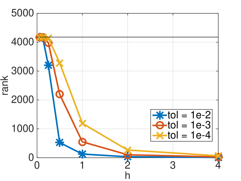
(a) Numerical ranks

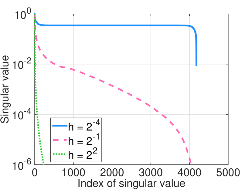
(b) Singular value decay

Figure 1: Numerical ranks of the kernel matrix versus $h$. The data used is Abalone, and is normalized in each dimension. The numerical rank is computed as $\text{argmin}_{k}(\sigma_{k}<tol\cdot\sigma_{1})$, where $\sigma_{1}\geq\sigma_{2}\geq,\ldots,\geq\sigma_{n}$ are the singular values, and $tol$ is the tolerance. The plot on the right shows the decay patterns of singular values for varying $h$.

Low-rank matrix approximations are efficient in the large-$h$ regime, and in such regime, the matrix rank is low. Unfortunately, in the small-$h$ regime, they fall back to models with quadratic complexity. One natural question is whether the situation where a relatively small $h$ is useful occur in machine learning, or whether low-rank methods are sufficient. We answer this question in the following section, where we study kernel classifiers on real datasets and investigate the influence of $h$ on accuracy.

2.2 Optimal kernel bandwidth

We study the optimal bandwidth parameters used in practical situations, and in particular, we consider kernel classifiers. In practice, the parameter $h$ is selected by a cross-validation procedure combined with a grid search, and we denote such parameter as $h_{CV}$. For datasets with wide intra-variability, we observed that the optimal parameters of some small classes turned out to be smaller than $h_{CV}$. By small classes, we refer to those with fewer points or smaller diameters.

Table 1 lists some classification datasets with wide intra-variability. This class imbalance has motivated us to study the individual performance of each class. We found that there can be a significant discrepancy between $h_{CV}$ which is optimal overall for the entire dataset and the optimal $h$ for a specific class. In Figure 2, we used kernel SVM classifier under a wide range of $h$ and measure the performance by $F_{1}$ score on the test data. The $F_{1}$ score is the harmonic mean of the precision and recall, i.e.,

$$\frac{2\times\text{precision}\times\text{recall}}{\text{precision}+\text{recall}}.$$

The data was randomly divided into 80% training set and 20% testing set. Figure 2 shows the test $F_{1}$ score versus $h$ for selected classes. We see that for some smaller classes represented by darker colors, the $F_{1}$ score peaks at a value for $h$ that is smaller than $h_{CV}$. Specifically, for the smallest class (black curve) of each dataset, as $h$ increases from their own optimal $h$ to $h_{CV}$, the test $F_{1}$ scores drop by 21%, 100%, 16%, and 5% for EMG, CTG, Otto and Gesture datasets, respectively. To interpret the value of $h$ in terms of matrix rank, we plotted the singular values for different values of $h$ for the CTG and Gesture dataset in Figure 3. We see that when using $h_{CV}$, the numerical rank is much lower than using a smaller $h$ which leads to a better performance on smaller classes.

The above observation suggests that the value of $h_{CV}$ is mostly influenced by large classes and using $h_{CV}$ may degrade the performance of smaller classes. Therefore, to improve the prediction accuracy for smaller classes, one way is to reduce the bandwidth $h$. Unfortunately, a decrease in $h$ increases the rank of the corresponding kernel matrix, making low-rank algorithms inefficient. Moreover, even if we create the model using $h_{CV}$, as discussed previously, the rank of the kernel matrix will not be very low in most cases. These altogether stress the importance of developing an algorithm that extends the domain of applicability of low-rank algorithms.

Table 1: Statistics for classification datasets and their selected classes, $r_{i}$ is the median distance to the center for class $i$, $n_{i}$ is the number of points in class $i$.

Data	n	d		Selected Classes    (other classes not shown)
				1	2	3	4	5
EMG	28,500	8	$n_{i}$	1,500	1,500	1,500	1,500	1,500
			$r_{i}^{2}$	$\bf 1.3\times 10^{-4}$	$2.9\times 10^{-3}$	$2.6\times 10^{-2}$	$4.5\times 10^{-1}$	$\bf 2.6\times 10^{0}$
CTG	2,126	23	$n_{i}$	51	71	241	318	555
			$r_{i}^{2}$	1.0	1.2	1.4	1.3	1.4
Gesture	9,873	32	$n_{i}$	2,741	998	2,097	1,087	2,948
			$r_{i}^{2}$	$\bf 1.8\times 10^{-2}$	$2.7\times 10^{-2}$	$1.4\times 10^{-1}$	$1.9\times 10^{-1}$	$\bf 2.3\times 10^{-1}$
Otto	20,000	93	$n_{i}$	625	870	1602	2736	4570
			$r_{i}^{2}$	0.26	0.40	0.46	0.45	0.64

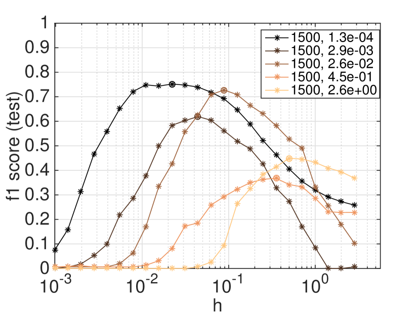
(a) EMG, $h_{CV}=0.17$

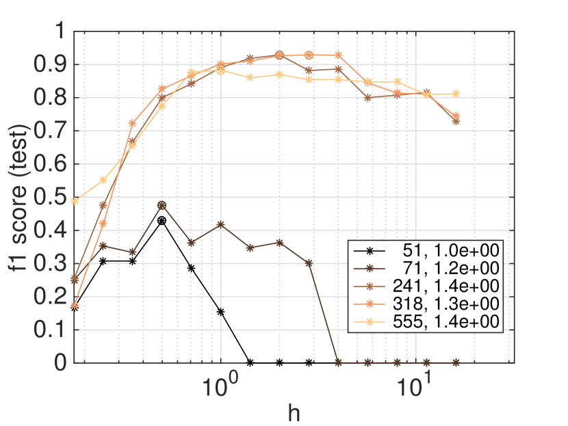
(b) CTG, $h_{CV}=1.42$

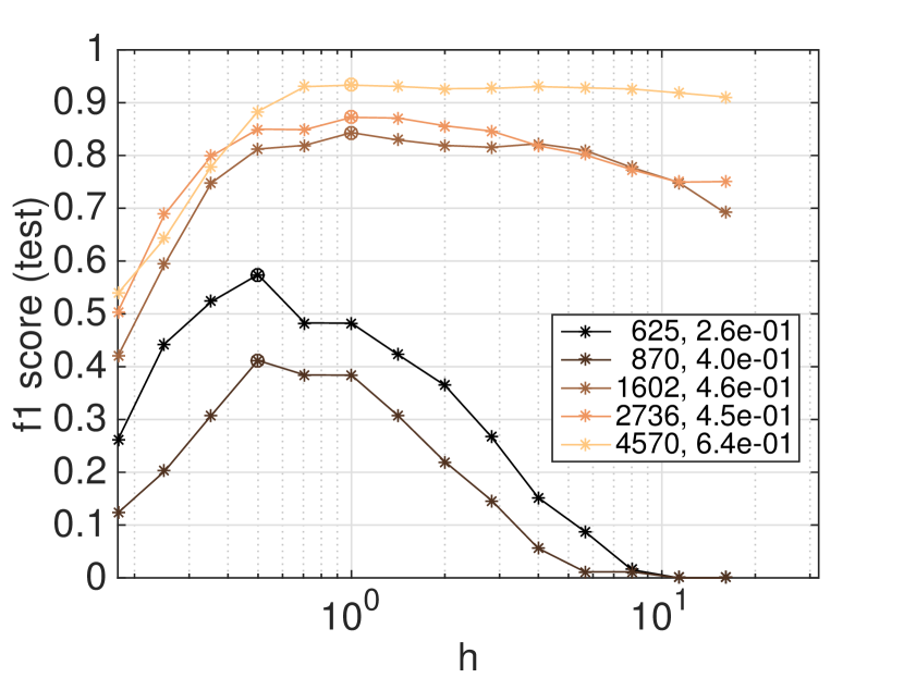
(c) Otto, $h_{CV}=1$

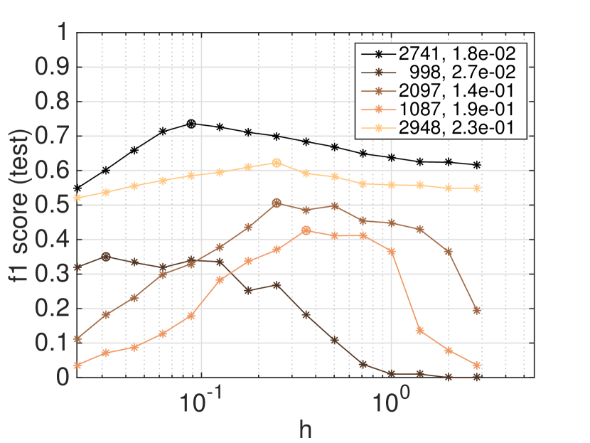
(d) Gesture, $h_{CV}=0.25$

Figure 2: Test $F_{1}$ score of selected class for different datasets. Each curve represents one class, and the solid circle represents the maximum point along the curve. The legend represents a pair ($n_{i},r_{i}^{2}$), where $n_{i}$ is the number of point in each class, $r_{i}$ is the median distance to class center. $h_{CV}$ is the parameter obtained from cross-validation. We see that for smaller classes (represented by darker colors), the $F_{1}$ score peaks at an $h$ that is smaller than $h_{CV}$.

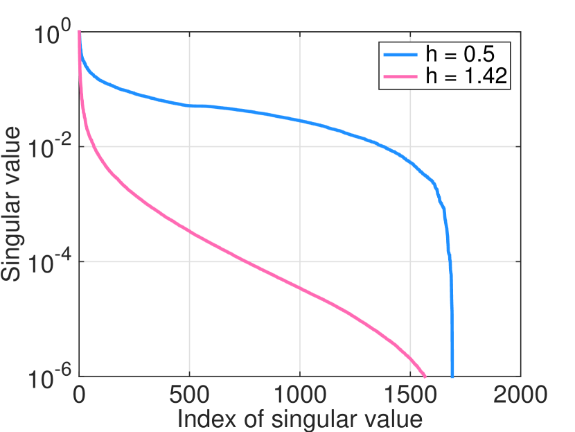
(a) CTG

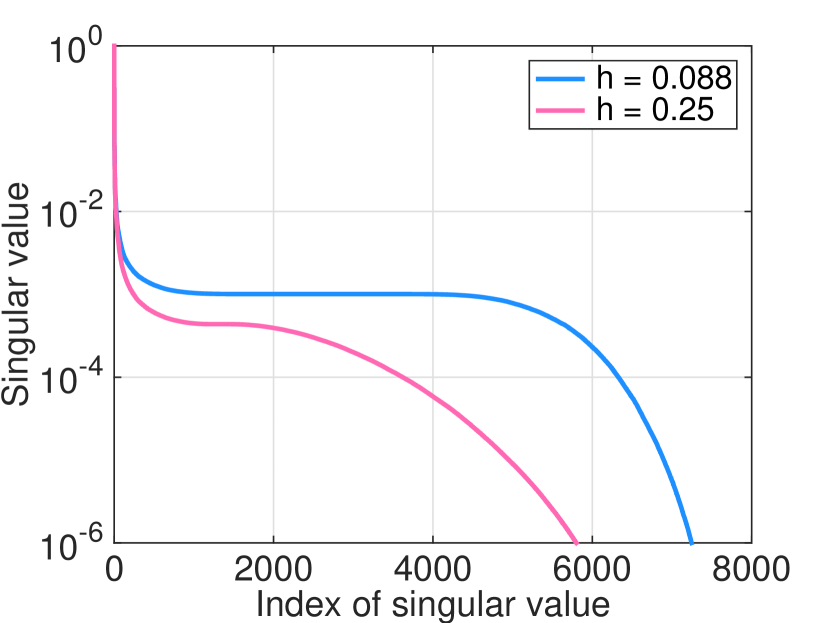
(b) Gesture

Figure 3: Singular value decay for CTG dataset and Gesture dataset on selected bandwidths. In subplot (a), $h_{CV}=1.42$ and $h=0.5$, respectively, is the optimal paraemter for the full dataset and the smallest dataset. In subplot (b), $h_{CV}=0.25$ is the optimal parameter for the full dataset, and $h=0.088$ achieves a good $F_{1}$ score for clusters of small radii.

2.3 Factors affecting the optimal kernel bandwidth

This section complements the previous section by investigating some data properties that influence the optimal kernel bandwidth parameter $h$.

We studied synthetic two-dimensional data and our experiments suggested that the optimal $h$ depends strongly on the smallest radius of curvature of the decision surface (depicted in Figure 4). By optimal we mean the parameter that yields the highest accuracy, and if multiple such parameters exist, we refer to the largest one to be optimal and denote it as $h^{*}$.

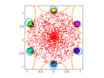
Figure 4: Decision boundary with varying smallest radius of curvatures. Dots represent data points and different classes are color coded. The curves represent the decision boundaries, of which the radii of curvature are large, median, and small for the orange, blue and black (those surrounding the small clusters) curves, respectively.

We first experimentally study the relation between $h^{*}$ and the smallest radius of curvature of the decision boundary. Figure 5 shows Gaussian clusters with alternating labels that are color coded. We decrease the radius of curvature of the decision boundary by decreasing the radius of each cluster while keeping the box size fixed. We quantify the smallest radius of curvature of the decision boundary approximately by the standard deviation $\sigma$ of each cluster. Figure 5b shows a linear correlation between $\sigma$ and $h^{*}$.

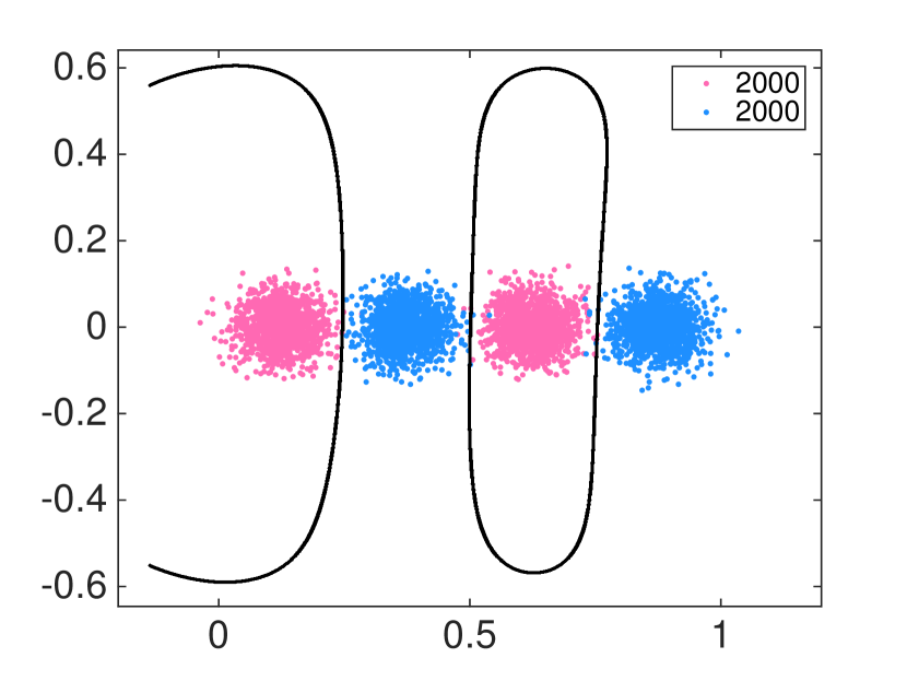
(a) Data with 4 clusters

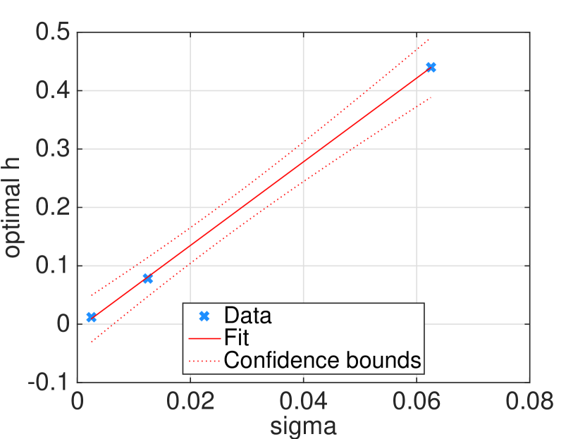
(b) Relation of $\sigma$ and optimal $h$

Figure 5: Left: Data (4 clusters) with two alternating labels (20 and 100 clusters cases are not shown). Each cluster is generated from a Gaussian distribution with standard deviation $\sigma$. The decision boundary (black curve) is associated with $h^{*}=0.44$. Right: Linear relation of the standard deviation $\sigma$ ($\approx$ half of cluster radius) of each cluster and $h^{*}$.

We study a couple more examples. Figure 6 shows two smaller circles with different radii surrounded by a large circle. For this example, the smallest radius of curvature of the decision boundary depends strongly on the cluster radius. Hence, the optimal $h$ for the smaller class (pink colored) should be smaller than that for the larger class (orange colored), which was verified by the $F_{1}$ score. Compared to the large cluster, the $F_{1}$ score for the small cluster peaks at a smaller $h$ and drops faster as $h$ increases. A similar observation was made in higher-dimensional data as well. We generated two clusters of different radii which are surrounded by a larger cluster in dimension 10. Figure 7 shows that the intuition in dimension 2 nicely extends to dimension 10. Another cluster example is in Figure 4, which shows multiple small clusters overlapping with a larger cluster at the boundary. The 3 reference decision boundaries correspond to $h$ being 1.5 (orange), 0.2 (blue) and 0.02 (black), respectively. The highest accuracy was achieved at $h=0.5$, which is close to the small cluster radius 0.2 and is large enough to tolerate the noises in the overlapping region.

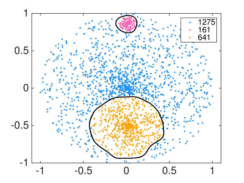
(a) Data and decision boundary

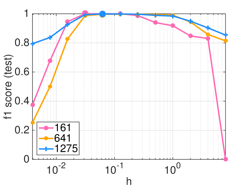
(b) $F_{1}$ score for test data

Figure 6: Left: classes surrounded by a larger one; the legend shows the number of points in each class. The decision boundary (black curve) is for $h=0.125$. Right: the test $F_{1}$ score for the test data versus $h$.

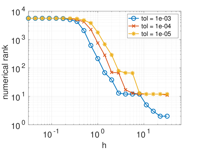
(a) Numerical ranks

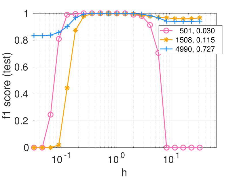
(b) $F_{1}$ score for test data

Figure 7: Left: numerical ranks of the kernel matrix evaluated on the training data versus $h$. Right: the $F_{1}$ score for the test data versus $h$. The synthetic data is in dimension 10 and has three clusters of different radii. The legend represents a pair $(n_{i},r_{i})$, where $n_{i}$ is the number of points in cluster $i$ and $r_{i}$ is the cluster radius.

The above examples, along with many that are not shown in this paper, have experimentally suggested that the optimal parameter $h$ and the smallest radius of curvature of the decision surface are positively correlated. Hence, for datasets whose decision surfaces are highly nonlinear, i.e., of small radius of curvature, a relatively small $h$ is very likely needed to achieve a high accuracy.

In the following section, we will introduce our novel scheme to accelerate kernel evaluations, which remains efficient in cases where traditional low-rank methods are inefficient.

3 Block Basis Factorization

In this section, we propose the Block Basis Factorization (BBF) that extends the availability of traditional low-rank structures. subsection 3.1 describes the BBF structure. subsection 3.2 proposes its fast construction algorithm.

3.1 BBF Structure

This section defines and analyzes the Block Basis Factorization (BBF). Given a symmetric matrix $M\in\mathbb{R}^{n\times n}$ partitioned into $k$ by $k$ blocks, let $M_{i,j}$ denote the $(i,j)$-th block for $i,j=1,\ldots,k$. Then, the BBF of $M$ is defined as:

(1) $$M=\widetilde{U}\widetilde{C}\widetilde{U}^{\top},$$

where $\widetilde{U}$ is a block diagonal matrix with the $i$-th diagonal block $U_{i}$ being the column basis of $M_{i,j}$ for all $j$, and $\widetilde{C}$ is a $k$ by $k$ block matrix with the $(i,j)$-th block denoted by $C_{i,j}=U_{i}^{\top}M_{i,j}U_{j}$. The BBF structure is depicted in Figure 8.

$=$

Figure 8: $M=\widetilde{U}\widetilde{C}\widetilde{U}^{\top}$

We discuss the memory cost for the BBF structure. If the numerical ranks of all the base $U_{i}$ are bounded by $r$, then the memory cost for the BBF is $O(nr+(rk)^{2})$. Further, if $k\leq\sqrt{n}$ and $r$ is a constant independent of $n$, then the BBF gives a data-sparse representation of matrix $M$. In this case, the complexity for both storing the BBF structure and applying it to a vector will be linear in $n$.

It is important to distinguish between our BBF and a block low-rank (BLR) structure [2]. There are two main differences: 1). The memory usage of the BBF is much less than BLR. BBF has one basis for all the blocks in the same row; while BLR has a separate basis for each block. The memory for BBF is $nr+(rk)^{2}$, whereas for BLR it is $2nkr$. 2). It is more challenging to construct BBF in linear complexity while remaining accurate. A direct approach using SVD to construct the low-rank base has a cubic cost; while a simple randomized approach would be inaccurate and unstable.

In the next section, we will propose an efficient method to construct the BBF structure, which uses randomized methods to reduce the cost while still providing a robust approach. Our method is linear in $n$ for many kernels used in machine learning applications.

3.2 Fast construction algorithm for BBF

In this section, we first introduce a theorem in subsubsection 3.2.1 that reveals the motivation behind our BBF structure and addresses the applicable kernel functions. We then propose a fast construction algorithm for BBF in subsubsection 3.2.2.

3.2.1 Motivations

Consider a RBF kernel function $\mathcal{K}:\mathbb{R}^{d}\times\mathbb{R}^{d}\mapsto\mathbb{R}$. The following theorem in [39] provides an upper bound on the error for the low-rank representation of kernel $\mathcal{K}$. The error is expressed in terms of the function smoothness and the diameters of the source domain and the target domain.

Theorem 3.1.

Consider a function $f$ and kernel $\mathcal{K}({\bf x},{\bf y})=f(\lVert{\bf x}-{\bf y}\rVert_{2}^{2})$ with ${\bf x}=(x_{1},\ldots,x_{d})$ and ${\bf y}=(y_{1},\ldots,y_{d})$. We assume that $x_{i}\in[0,D/\sqrt{d}]$, $y_{i}\in[0,D/\sqrt{d}]$, where $D$ is a constant independent of $d$. This implies that $\|{\bf x}-{\bf y}\|_{2}^{2}\leq D^{2}$. We assume further that there are $D_{\bf x}<D$ and $D_{\bf y}<D$, such that $\|{\bf x}_{i}-{\bf x}_{j}\|_{2}\leq D_{\bf x}$ and $\|{\bf y}_{i}-{\bf y}_{j}\|_{2}\leq D_{\bf y}$.

Let $f_{p}(x)=\sum_{n}\mathcal{T}\circ f(x+4nD^{2})$ be a $4D^{2}$-periodic extension of $f(x)$, where $\mathcal{T}(\cdot)$ is 1 on $[-D^{2},D^{2}]$ and smoothly decays to 0 outside of this interval. We assume that $f_{p}$ and its derivatives through $f_{p}^{(q-1)}$ are continuous, and the $q$-th derivative is piecewise continuous with its total variation over one period bounded by $V_{q}$.

Then, $\forall\leavevmode\nobreak\ M_{f},M_{t}>0$ with $9M_{f}\leq M_{t}$, the kernel $\mathcal{K}$ can be approximated in a separable form whose rank is at most $R=R(M_{f},M_{t},d)=4M_{f}\binom{M_{t}+d}{d}$

$$\mathcal{K}({\bf x},{\bf y})=\sum_{i=1}^{R}g_{i}({\bf x})h_{i}({\bf y})+\epsilon_{M_{f},M_{t}}$$

The $L_{\infty}$ error is bounded by

$$|\epsilon_{M_{f},M_{t}}|\leq\lVert f\rVert_{\infty}\left(\frac{D_{\bf x}D_{\bf y}}{D^{2}}\right)^{M_{t}+1}+\frac{V_{q}}{\pi q}\left(\frac{2D^{2}}{\pi M_{f}}\right)^{q}.$$

In Theorem 3.1, the error is up bounded by the summation of two terms. We first study the second term, which is independent of $D_{\bf x}$ or $D_{\bf y}$. The second term depends on the smoothness of the function, and decays exponentially as the smoothness of the function increases. Many kernel functions used in machine learning are sufficiently smooth; hence, the second term is usually smaller than the first term. Regarding the first term, the domain diameter information influences the error through the factor $\left(\frac{D_{\bf x}D_{\bf y}}{D^{2}}\right)^{M_{t}+1}$, which suggests for a fixed rank (positively related to $M_{t}$), reducing either $D_{\bf x}$ or $D_{\bf y}$ reduces the error bound. It also suggests that for a fixed error, reducing either $D_{\bf x}$ or $D_{\bf y}$ reduces the rank. This has motivated us to cluster points into distinct clusters of small diameters, and by the theorem, the rank of the submatrix that represents the local interactions from one cluster to the entire dataset would be lower than the rank of the entire matrix.

Hence, we seek linear-complexity clustering algorithms that are able to separate points into clusters of small diameters. $k$-means and $k$-centers algorithms are natural choices. Both algorithms partition $n$ data points in dimension $d$ into $k$ clusters at a cost of $O(nkd)$ per iteration. Moreover, they are based on the Euclidean distance between points, which is consistent with the RBF kernels which are functions of the Euclidean distance. In practice, the algorithms converge to slightly different clusters due to different objective functions, but neither is absolutely superior. Importantly, the clustering results from these algorithms yield a more memory efficient BBF structure than random clusters. A more task-specific clustering algorithm will possibly yield better result; however, the main focus of this paper is on factorizing the matrix efficiently, rather than proposing new approaches to identify good clusters.

We experimentally verify our motivation on a real-world dataset. We clustered the pendigits dataset into 10 clusters ($C_{1},C_{2},\ldots,C_{10}$) using the $k$-means algorithm, and reported the statistics of each cluster in 9(a). We see that the radius of each cluster is smaller than that of the full dataset. We further plotted the normalized singular values of the entire matrix $M$ and its sub-matrices $M(C_{i},:)$ in 9(b). Notably, the normalized singular value of the sub-matrices shows a significantly faster decay than that of the entire matrix. This suggests that the ranks of sub-matrices are much lower than that of the entire matrix. Hence, by clustering the data into clusters of smaller radius, we are able to capture the local interactions that are missed by the conventional low-rank algorithms which only consider global interactions. As a result, we achieve a similar level of accuracy with a much less memory cost.

Cluster	Radius	Size
1	42.4	752
2	41.3	603
3	37.6	729
4	24.3	733
5	24.2	1571
6	23.0	588
7	21.8	1006
8	21.6	421
9	21.4	236
10	21.3	855
Full	62.8	7494

(a)

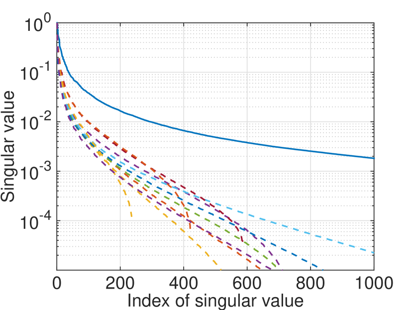
(b)

Figure 9: Left (a): Clustering result of the pendigits dataset. Right (b): Normalized singular value decay. In subplot (b), the solid curve represents the entire matrix $M$, and the dash curves represent the row-submatrices $M(C_{i},:)$. The kernel used was the Gaussian kernel with bandwidth parameter $h=2$.

3.2.2 BBF Construction Algorithm

This section proposes a fast construction algorithm for the BBF structure. For simplicity, we assume the data points are evenly partitioned into $k$ clusters, $\mathcal{C}_{1},\dots,\mathcal{C}_{k}$, and the numerical rank for each submatrix is $r$. We first permute the matrix according to the clusters:

(2) $$M=PKP^{\top}=\bordermatrix{{}&\mathcal{C}_{1}&\mathcal{C}_{2}&\cdots&\mathcal{C}_{k}\cr\mathcal{C}_{1}&M_{1,1}&M_{1,2}&\cdots&M_{1,k}\cr\mathcal{C}_{2}&M_{2,1}&M_{2,2}&\cdots&M_{2,k}\cr\vdots&\vdots&\vdots&\ddots&\vdots\cr\mathcal{C}_{k}&M_{k,1}&M_{k,2}&\cdots&M_{k,k}},$$

where $P$ is a permutation matrix, and $M_{i,j}=\mathcal{K}(\mathcal{C}_{i},\mathcal{C}_{j})$ is the interaction matrix between cluster $\mathcal{C}_{i}$ and cluster $\mathcal{C}_{j}$.

Our fast construction algorithm consists of two components: basis construction and inner matrix construction. In the following, we adopt Matlab’s notation for submatrices. We use the colon to represent 1:end, e.g., $M_{i,:}=\begin{pmatrix}M_{i,1}&\cdots&M_{i,k}\end{pmatrix}$, and use the index vectors $\mathcal{I}$ and $\mathcal{J}$ to represent sub-rows and sub-columns, e.g., $M(\mathcal{I},\mathcal{J})$ represents the intersection of rows and columns whose indices are $\mathcal{I}$ and $\mathcal{J}$, respectively.

1. Basis construction

We consider first the basis construction algorithm. The most accurate approach is to explicitly construct the submatrix $M_{i,:}$ and apply an SVD to obtain the column basis; regrettably, it has a cubic cost to compute all the bases. Randomized SVD [27] reduces the cost to quadratic while being accurate; however, a quadratic complexity is still expensive in practice. In the following, we describe a linear algorithm that is accurate and stable. Since the proposed algorithm adopts randomness, by “stable” we mean the variance of the output is small under multiple runs. The key idea is to restrict us in a subspace by sampling columns of large volume.

The algorithm is composed of two parts. In the first part, we select some columns of $M_{i,:}$ that are representative of the column space. By representative, we mean the $r$ sampled columns have volume approximating the maximum $r$-dimensional volume among all column sets of size $r$. In the second part, we apply the randomized SVD algorithm to the representative columns to extract the column basis.

Part 1: Randomized sampling algorithm

We seek a sampling method that samples columns with approximate maximum volume. Strong rank revealing QR (RRQR) [23] returns columns whose volume is proportional to the maximum volume obtained by SVD. QR with column pivoting (pivoted QR) is a practical replacement for the strong RRQR due to its inexpensive computational cost. To ensure a linear complexity, we use the pivoted QR factorization with a randomized approach.

We describe the randomized sampling method [16] used in our BBF algorithm; the algorithm detail is in algorithm 1 with the procedure depicted in Figure 10. The complexity of sampling $r$ columns from an $m\times n$ matrix is $O(r^{2}(m+n))$. The size of the output index sets $\Pi_{r}$ and $\Pi_{c}$ could grow as large as $qr$, but it can be controlled by some practical algorithmic modifications. One is that given a tolerance, we truncate the top columns based on the magnitudes of the diagonal entries of matrix $R$ from the pivoted QR. Another is to apply an early stopping once the important column index set do not change for two consecutive iterations. For the numerical results reported in this paper, we used $q=2$. Note that any linear sampling algorithm can substitute algorithm 1, and in practice, algorithm 1 returns columns whose volume is very close to the largest.

1 Function Randomized_Sampling($M_{i,:}$, $r_{i}$, $q$)

2      

      input : (1) Row-submatrix $M_{i,:}$ to sample from in its implicit form (given data and kernel function); (2) Sample size $r_{i}$; (3) Iteration parameter $q$

3      

      output : Important column index set $\Pi_{c}$ for $M_{i,:}$

4      

5      $\Pi_{r}=\emptyset$

6      

7      for iter=1, …, $q$ do

8             Important columns. Uniformly sample $r_{i}$ rows, and denote the index set as $\Gamma_{r}$, update $\Pi_{r}=\Pi_{r}\cup\Gamma_{r}$. Apply a pivoted QR factorization on $M_{i,:}(\Pi_{r},:)$ to get the important columns index set, denoted as $\Pi_{c}$.

9            

10            Important rows. Uniformly sample $r_{i}$ columns, and denote the index set as $\Gamma_{c}$. Update $\Pi_{c}=\Gamma_{c}\cup\Pi_{c}$. Apply a pivoted LQ factorization on $M_{i,:}(:,\Pi_{c})$ to get the important row index set, denoted as $\Pi_{r}$.

11            

12       end for

13      

14      return $\Pi_{c}$

15

16Note: The pivoted QR is the QR factorization with column pivoting based on the largest column norm.

17

Algorithm 1 Randomized sampling algorithm for each submatrix

1 Function BBF_Sampling($\{M_{i,:}\}_{i=1}^{k}$, $\{r_{i}\}_{i=1}^{k}$, $q$)

2      

      input : (1) Sub-matrices $\{M_{i,:}\}_{i=1}^{k}$ to sample from in their implicit forms (given data and kernel function); (2) Sample sizes $\{r_{i}\}_{i=1}^{k}$ for each sub-matrix $M_{i,:}$; (3) Iteration parameter $q$

3      

      output : Important column index set $\Pi_{i}$ for each row-submatrix

4      

5      for $i=1,\ldots,k$ do

6             $\Pi_{i}$ = Randomized_Sampling($M_{i,:}(:,\Gamma),r_{i},q)$ (using algorithm 1)

7       end for

8      

9      return $\Pi_{i}$ for $i=1,\ldots,k$

10

Algorithm 2 BBF sampling algorithm

Applying algorithm 1 to $k$ submatrices $\{M_{i,:}\}_{i=1}^{k}$ will return the desired $k$ sets of important columns for BBF, which is described in algorithm 2. The complexity of algorithm 2 depends on $k$ (see subsubsection 3.2.3 for details), and we can remove this dependence by applying algorithm 1 on a pre-selected and refined set of columns instead of all the columns. This leads to a more efficient procedure to sample columns for the $k$ submatrices as described in algorithm 3. Our final BBF construction algorithm will use algorithm 2 for column sampling.

1 Function BBF_Sampling_I($\{M_{i,:}\}_{i=1}^{k}$, $\{r_{i}\}_{i=1}^{k}$, $q$)

2      

      input : (1) Sub-matrices $\{M_{i,:}\}_{i=1}^{k}$ to sample from in their implicit forms (given data and kernel function); (2) Sample sizes $\{r_{i}\}_{i=1}^{k}$ for each sub-matrix $M_{i,:}$; (3) Iteration parameter $q$

3      

      output : Important column index set $\Pi_{i}$ for each row-submatrix

4      

5      for $i=1,\ldots,k$ do

6             Randomly sample $r_{i}$ columns from $M_{i}$ and denote the index set as $\Pi_{i}$

7            

8            Apply a pivot LQ on $M_{i,:}(:,\Pi_{i})$ to obtain $r$ important rows, and we denote the index set as $\Gamma_{i}$

9       end for

10      

11      Stack all the sampled rows $\Gamma=[\Gamma_{1},\ldots,\Gamma_{k}]$

12      

13      for $i=1,\ldots,k$ do

14             $\Pi_{i}$ = Randomized_Sampling($M_{i,:}(:,\Gamma),r_{i},q)$ (using algorithm 1)

15       end for

16      

17      return $\Pi_{i}$ for $i=1,\ldots,k$

18

Algorithm 3 More efficient BBF sampling algorithm

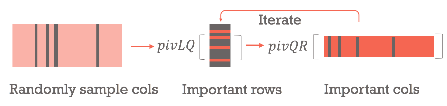
Figure 10: A pictorial description of the sampling algorithm. We start with sampling random columns, and iterate between important rows (by pivoted LQ) and important columns (by pivoted QR) to obtain our refined important columns. This procedure is usually repeated for a few times to ensure the stability of the important indices.

Part 2: Orthogonalization algorithm

Having sampled the representative columns $M_{i,:}(:,\Pi_{i})$, the next step is to obtain the column basis that approximates the span of the selected columns. This can be achieved through any orthogonalization methods, e.g., pivoted QR, SVD, randomized SVD [27], etc. According to algorithm 1, the size of the sampled index set $\Pi_{c}$ can be as large as $qr$. In practice, we found that the randomized SVD works efficiently. The randomized SVD algorithm was proposed to reduce the cost of computing a rank-$r$ approximation of an $m\times n$ matrix to $O(mnr)$. The algorithm is described in algorithm 4. The practical implementation of algorithm 4 involves an oversampling parameter $\ell$ to reduce the iteration parameter $q$. For simplicity, we eliminate $\ell$ from the pseudo code.

1 Function  Randomized_SVD($M$, $r$, $q$)

2      

      input : (1) Matrix $M\in\mathbb{R}^{m\times n}$; (2) desired rank $r$; (3) iteration parameter $q$

3      

      output : $U$, $\Sigma$, and $V$ such that $M\approx U\Sigma V^{\top}$

4      

5      Randomly generate a Gaussian matrix $\Omega\in\mathbb{R}^{n\times r}$

6      

7      $M\Omega$ = $QR$

8      

9      for $i$=1, …, $q$ do

10             $M^{\top}Q=\hat{Q}\hat{R}$

11             $M\hat{Q}=QR$

12       end for

13      

14      $\hat{U}\Sigma V^{\top}=Q^{\top}M$

15      

16      $U=Q\hat{U}$

17      return $U$, $\Sigma$, $V$

18

Algorithm 4 Randomized SVD

2. Inner matrix construction

We then consider the inner matrix construction. Given column base $U_{i}$ and $U_{j}$, we seek a matrix $C_{i,j}$ such that it minimizes

$$\|M_{i,j}-U_{i}C_{i,j}U_{j}^{\top}\|.$$

The minimizer is given by $C_{i,j}=U_{i}^{\dagger}M_{i,j}(U_{j}^{\top})^{\dagger}$. Computing $C_{i,j}$ exactly has a quadratic cost. Again, we restrict ourselves in a subspace and propose a sampling-based approach that is efficient yet accurate. The following proposition provides a key theoretical insight behind our algorithm.

Proposition 3.2.

If a matrix $M\in\mathbb{R}^{m\times n}$ can be written as $M=UCV^{\top}$, where $U\in\mathbb{R}^{m\times r}$ and $V\in\mathbb{R}^{n\times r}$. Further, if for some index set $\mathcal{I}$ and $\mathcal{J}$, $U(\mathcal{I},:)$ and $V(\mathcal{J},:)$ are full rank, then, the inner matrix $C$ is given by

(3) $$C=(U(\mathcal{I},:))^{\dagger}\;M(\mathcal{I},\mathcal{J})\;(V(\mathcal{J},:)^{\top})^{\dagger},$$

where $\dagger$ denotes the pseudo-inverse of the matrix.

Proof 3.3.

To simplify the notations, we denote $\widehat{U}=U(\mathcal{I},:)$, $\widehat{V}=V(\mathcal{J},:)$, and $\widehat{M}=M(\mathcal{I},\mathcal{J})$, where $\mathcal{I}$ is the sampled row index set for $U$ and $\mathcal{J}$ is the sampled row index set for $V$. We apply the sampling matrices $P_{\mathcal{I}}$ and $P_{\mathcal{J}}$ (matrices of 0’s and 1’s) to both sides of equation $M=UCV^{\top}$, and obtain

$$P_{\mathcal{I}}MP_{\mathcal{J}}^{\top}=P_{\mathcal{I}}UCV^{\top}P_{\mathcal{J}}^{\top},$$

i.e.,

$$\widehat{M}=\widehat{U}C\widehat{V}^{\top}.$$

The assumption that $\widehat{U}$ and $\widehat{V}$ are tall and skinny matrices with full column ranks implies that $\widehat{U}^{\dagger}\hat{U}=I$ and $\widehat{V}^{\top}(\widehat{V}^{\top})^{\dagger}=I$. We then multiply $\widehat{U}^{\dagger}$ and $(\widehat{V}^{\top})^{\dagger}$ on both sides and obtain the desired result:

$$\widehat{U}^{\dagger}\widehat{M}(\widehat{V}^{\top})^{\dagger}=\widehat{U}^{\dagger}\widehat{U}C\widehat{V}^{\top}(\widehat{V}^{\top})^{\dagger}=C.$$

Prop. 3.2 provides insights into an efficient, stable and accurate construction of the inner matrix. In practice, the equality $M=UCV^{\top}$ in Prop. 3.2 often holds with an error term and we seek index sets $\mathcal{I}$ and $\mathcal{J}$ such that the computation for $C$ is accurate and numerically stable. Equation 3 suggests that a good choice leads to an $M(\mathcal{I},\mathcal{J})$ with a large volume. However, finding such a set can be computationally expensive and a heuristic is required for efficiency. We used a simplified approach where we sample $\mathcal{I}$ (resp. $\mathcal{J}$) such that $U(\mathcal{I},:)$ (resp. $V(\mathcal{J},:)$) has a large volume. This leads to good numerical stability, because having a large volume is equivalent to being nearly orthogonal, which implies a good condition number. In principle, a pivoted QR strategy could be used but, fortunately, we are able to skip it by using the results from the basis construction. Recall that in the basis construction, the important rows were sampled using a pivoted LQ factorization, hence, they already have large volumes.

Therefore, the inner matrix construction is described in what follows. We first uniformly sample $r$ column indices $\Gamma_{j}$ and $r$ row indices $\Gamma_{i}$, respectively, from $\mathcal{C}_{j}$ and $\mathcal{C}_{i}$. Then, the index sets are constructed as $\mathcal{I}=\Pi_{i}\cup\Gamma_{i}$ and $\mathcal{J}=\Pi_{j}\cup\Gamma_{j}$, where $\Pi_{i}$ and $\Pi_{j}$ are the important row index sets from the basis construction. Finally, $C_{i,j}$ is given by

$$(U_{i}(\mathcal{I},:))^{\dagger}\;M_{i,j}(\mathcal{I},\mathcal{J})\;(U_{j}(\mathcal{J},:)^{\top})^{\dagger}.$$

We also observed small entries in some off-diagonal blocks of the inner matrix. Those blocks normally represent far-range interactions. We can set the blocks for which the norm is below a preset threshold to 0. In this way, the dense inner matrix becomes a block-wise sparse matrix, further reducing the memory.

Having discussed the details for the construction algorithm, we summarize the procedure in algorithm 5, which is the algorithm used for all the numerical results.

1 Function BBF_Construction ($k$, $\{\mathcal{C}_{i}\}_{i=1}^{k}$, $\{r_{i}\}_{i=1}^{k}$, $M$, $q_{\text{Samp}}$, $q_{\text{SVD}}$)

2      

      Input : (1) Number of clusters $k$; (2) Clustering assignments $\{\mathcal{C}_{i}\}_{i=1}^{k}$; (3) Rank $\{r_{i}\}_{i=1}^{k}$ for each column basis; (4) Matrix $M$ in its implicit form; (5) Iteration parameter $q_{\text{Samp}}$ for randomized sampling; (6) Iteration parameter $q_{\text{SVD}}$ for randomized SVD.

3      

      Output : Block diagonal matrix $\widetilde{U}$ and block-wise sparse matrix $\widetilde{C}$ s.t. $M\approx\widetilde{U}\widetilde{C}\widetilde{U}^{\top}$

4      

5      $[\Pi_{1},\cdots,\Pi_{k}]$ = BBF_Sampling($\{M_{i,:}\}_{i=1}^{k}$, $\{r_{i}\}_{i=1}^{k}$, $q_{\text{Samp}}$) (algorithm 2)

6      

7      for $i=1,\ldots,k$ do

8             $U_{i}=$ Randomized_SVD($M_{i:}(:,\Pi_{i})$, $r_{i}$, $q_{\text{SVD}}$) (algorithm 4)

9       end for

10      

11      for $i=1,\ldots,k$ do

12             for $j=1,\ldots,i$ do

13                   if cutoff criterion is not satisfied then

14                         Uniformly sample $\Gamma_{i}$ and $\Gamma_{j}$ from $\mathcal{C}_{i}$ and $\mathcal{C}_{j}$, respectively

15                        

16                        $\mathcal{I}=\Pi_{i}\cup\Gamma_{i}$ and $\mathcal{J}=\Pi_{j}\cup\Gamma_{j}$

17                        

18                        $C_{i,j}=(U_{i}(\mathcal{I},:))^{\dagger}M_{i,j}(\mathcal{I},\mathcal{J})(U_{j}(\mathcal{J},:)^{\top})^{\dagger}$

19                        

20                        $C_{j,i}=C_{i,j}^{\top}$

21                  else

22                         $C_{i,j}=0$

23                         $C_{j,i}=0$

24                   end if

25                  

26             end for

27            

28       end for

29      

30      return $\tilde{U}$, $\tilde{C}$

31

Algorithm 5 Main Algorithm — Fast construction algorithm for BBF

In this section, for simplicity, we only present BBF for symmetric kernel matrices. However, the extension to general non-symmetric cases is straightforward by applying similar ideas, and the computational cost will be roughly doubled. Asymmetric BBF can be useful in compressing the kernel matrix in the testing phase.

3. Pre-computation: Parameter Selection

We present a heuristic algorithm to identify input parameters for BBF. The algorithm takes $n$ input points $\{{\bf x}_{i}\}_{i=1}^{n}$ and a requested error (tolerance) $\epsilon$, and outputs the suggested parameters for the BBF construction algorithm, specifically, the number of clusters $k$, the index set for each cluster $\mathcal{I}$, and the estimated rank $r_{i}$ for the submatrix corresponding to the cluster $\mathcal{I}$. We seek a set of parameters that minimizes the memory cost while keeping the approximation error below $\epsilon$.

Choice of column ranks. Given the tolerance $\epsilon$ and the number of clusters $k$, we describe our method of identifying the column ranks. To maintain a low cost, the key idea is to consider only the diagonal blocks instead of the entire row-submatrices. For each row-submatrix in the RBF kernel matrices (after permutation), the diagonal block, which represents the interactions within a cluster, usually has a slower spectral decay than that of off-diagonal blocks which represent the interactions between clusters. Hence, we minimize the input rank for the diagonal block and use this as the rank for those off-diagonal blocks in the same row.

Specifically, we denote $\sigma_{1,i}\geq\sigma_{2,i}\geq\ldots\geq\sigma_{n_{i},i}$ as the singular values for $M_{i,i}$. Then for block $M_{i,i}\in\mathbb{R}^{n_{i}\times n_{i}}$, the rank $r_{i}$ is chosen as

$$r_{i}=\min\Big{\{}m\leavevmode\nobreak\ \mid\leavevmode\nobreak\ \sum_{p=m+1}^{n_{i}}\sigma_{p,i}^{2}<\frac{n_{i}^{2}}{n^{2}}\|M_{i,i}\|_{F}^{2}\leavevmode\nobreak\ \epsilon^{2}\Big{\}}.$$

Choice of number of clusters $\bm{k}$. Given the tolerance $\epsilon$, we consider the number of clusters $k$. For $k$ clusters, the upper bound on the memory usage of BBF is $\sum_{i=1}^{k}n_{i}r_{i}+\left(\sum_{i=1}^{k}r_{i}\right)^{2}$, where $r_{i}$ is computed as described above. Hence, the optimal $k$ is the solution to the following optimization problem

$$\text{minimize}_{k}\;\;g(k)=\sum_{i=1}^{k}n_{i}r_{i}+\left(\sum_{i=1}^{k}r_{i}\right)^{2}$$

$$\text{subj to}\;\;r_{i}=\min\Big{\{}m\leavevmode\nobreak\ |\leavevmode\nobreak\ \sum_{p=m+1}^{n_{i}}\sigma_{p}^{2}<\frac{n_{i}^{2}}{n^{2}}\|M_{i,i}\|_{F}^{2}\leavevmode\nobreak\ \epsilon^{2}\Big{\}},\;\;\forall i$$

We observed empirically that in general, $g(k)$ is close to convex in the interval $[1,O(\sqrt{n})]$, which enables us to perform a dichotomy search algorithm with complexity $O(\log n)$ for the minimal point.

3.2.3 Complexity Analysis

In this section, we analyze the algorithm complexity. We will provide detailed analysis on the factorization step including the basis construction and the inner matrix construction, and skip the analysis for the pre-computation step. We first introduce some notations.

Notations. Let $k$ denote the number of clusters, $\{n_{i}\}_{i=1}^{k}$ denote the number of point in each cluster, $\{r_{i}\}_{i=1}^{k}$ denote the requested rank for the blocks in the $i$-th submatrix, and $l$ denote the oversampling parameter.

Basis construction. The cost comes from two parts, the column sampling and the randomized SVD. We first calculate the cost for the $i$-th row-submatrix. For the column sampling, the cost is $n_{i}(r_{i}+l)^{2}+n(r_{i}+l)^{2}$, where the first term comes from the pivoted $LQ$ factorization, and the second term comes from the pivoted $QR$ factorization. For the randomized SVD, the cost is $n_{i}(r_{i}+l)^{2}$. Summing up the costs from all the submatrices, we obtain the overall complexity

$$O\left(\sum_{i=1}^{k}n_{i}(r_{i}+l)^{2}+n(r_{i}+l)^{2}+n_{i}(r_{i}+l)^{2}\right).$$

We simplify the result by denoting the maximum numerical rank of all blocks as $r$. Then, the above complexity is simplified to $O(nkr^{2})$.

Inner matrix construction. The cost for computing inner matrix $C_{i,j}$ with sampled $M_{i,j}$, $U_{i}$ and $U_{j}$ is $r_{i}^{2}r_{j}+r_{i}r_{j}^{2}$. Summing over all the $k^{2}$ blocks, the overall complexity is given by

$$\sum_{i=1}^{k}\sum_{j=1}^{k}r_{i}^{2}r_{j}+r_{i}r_{j}^{2}.$$

With the same assumptions as above, the simplified complexity is $O(k^{2}r^{3})$. Note that $k$ can reach up to $O(\sqrt{n})$ while still maintaining a linear complexity for this step.

Finally, we summarize the complexity of our algorithm in Table 2.

Table 2: Complexity table. $n$ is the total number of points, $k$ is the number of clusters, $r$ is the numerical rank for column basis.

Pre-computation		Factorization		Application
Each block	$O(n_{i}r^{2})$	Basis	$O(nkr^{2})$	$O(nr+(rk)^{2})$
Compute $g(k)$	$O(nr^{2})$	Inner matrix	$O(k^{2}r^{3})$
Total	$O(r^{2}n\log n)$	Total	$O(nkr^{2}+k^{2}r^{3})$

From Table 2, we note that the factorization and application cost (storage) depend quadratically on the number of clusters $k$. This suggests that a large $k$ will spoil the linearity of the algorithm. However, this may not be the case for most machine learning kernels, and we will discuss the influence of $k$ on three types of kernel matrices: 1) well-approximated by a low-rank matrix; 2) full-rank but approximately sparse; 3) full-rank and dense.

1. Well-approximated by a low-rank matrix. When the kernel matrix is well approximated by a low-rank matrix, $kr$ is up bounded by a constant (up to the approximation accuracy). In this case, both the factorization and application costs are linear.

2. Full-rank but approximately sparse. When the kernel matrix is full-rank ($kr=O(n)$) but approximately sparse, the application cost (storage) remains linear due to the sparsity. By “sparsity”, we mean that as $h$ decreases, the entries in the off-diagonal blocks of the inner matrices become small enough that setting them to 0 does not cause much accuracy loss. The factorization cost, however, becomes quadratic when using algorithm 2. One solution is to use algorithm 3 for column sampling, which removes the dependence on $k$, assuming $k<O(\sqrt{n})$.

3. Full-rank and dense. In this case, BBF would be sub-optimal. However, we experimentally observed that many kernel matrices generated by RBF functions with high dimensional data are in case 1 or 2.

In the end, we empirically verify the linear complexity of our method. Figure 11 shows the factorization time (in second) versus the number of data points on some real datasets. The trend is linear, confirming the linear complexity of our algorithm.

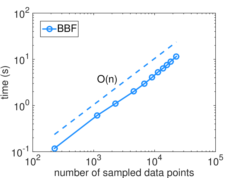
(a) Census housing, $h=2$

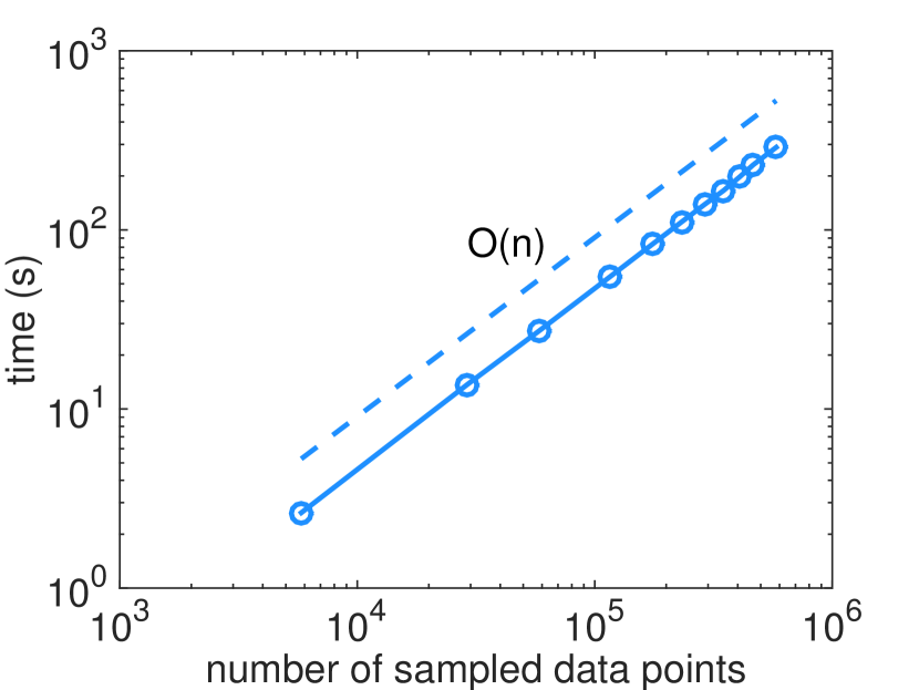
(b) Forest covertype, $h=2$

Figure 11: Factorization time (loglog scale) for kernel matrices from real datasets. To illustrate the linear growth of the complexity, we generated datasets with a varying number of points with the following strategy. We first clustered the data into 15 groups, and sampled a portion $p\%$ from each group, then increased $p$. To avoid the influence from other factors on the timing, we fixed the input rank for each block. As we can see, the timing grows linearly with the data size (matrix size).

4 Experimental Results

In this section, we experimentally verify the advantages of the BBF structure in subsection 4.1 and the BBF algorithm in subsection 4.2. By BBF algorithm we refer to the BBF structure and the proposed fast construction algorithm.

The datasets are listed in Table 3 and Table 1, and they can be downloaded from the UCI repository [6], the libsvm website [9] and Kaggle. All the data were normalized such that each dimension has mean 0 and standard deviation 1. All the experiments were performed on a computer with 2.4 GHz CPU and 8 GB memory.

Table 3: Real datasets used in the experiments.

Dataset	Abalone	Mushroom	Cpusmall
# Instance	4,177	8,124	8,192
# Attributes	8	112	16
Dataset	Pendigits	Census house	Forest covertype
# Instance	10,992	22,748	581,012
# Attributes	11	16	54

4.1 BBF structure

In this section, we will experimentally analyze the key factors in our BBF structure that contribute to its advantages over competing methods. Many factors contribute and we will focus our discussions on the following two: 1) The BBF structure has its column base constructed from the entire row-submatrix, which is an inherently more accurate representation than from diagonal blocks only (see MEKA); 2) The BBF structure considers local interactions instead of only global interactions used by a low-rank scheme.

4.1.1 Basis from the row-submatrix versus diagonal blocks

We verify that computing the column basis from the entire row-submatrix $M_{i,:}$ is generally more accurate than from the diagonal blocks $M_{i,i}$ only. Column basis computed from the diagonal blocks only preserves the column space information in the diagonal blocks, and will be less accurate in approximating the off-diagonal blocks. Figure 12 shows that computing the basis from the entire row-submatrix is more accurate.

a1 $M_{i,:}$, SVD

a2 $M_{i,i}$, SVD

b1 $M_{i,:}$, randomized

b2 $M_{i,i}$, randomized

Figure 12: Errors for each block in the approximated matrix from the Abalone dataset. Warmer color represents larger error. Subplot (a1) and (a2) shares the same colorbar; and (b1) and (b2) shares the same colorbar. The error for block $(i,j)$ is computed as $\|M_{i,j}-\widehat{M}_{i,j}\|_{F}/\|M\|_{F}$, where $\widehat{M}_{i,j}$ is the approximation of $M_{i,j}$. The basis in subplot (a1) and (a2) are computed by an SVD; and in (b1) and (b2) are computed by the randomized sampling algorithm. As we can see, computing the column basis from the diagonal blocks leads to lower error in the diagonal blocks; however, the errors in the off-diagonal blocks are much larger. The relative error in subplot (a1), (a2), (b1) and (b2) are $1.4\times 10^{-3}$, $6.3\times 10^{-3}$, $1.5\times 10^{-2}$, $4.0\times 10^{-2}$, respectively.

4.1.2 BBF structure versus low-rank structure

We compare the BBF structure and the low-rank structure. The BBF structure refers to Figure 8, and the low-rank structure means $K\approx UU^{\top}$, where $U$ is a tall and skinny matrix. For a fair comparison, we fixed all the factors to be the same except for the structure. For example, for both the BBF and the low-rank schemes, we used the same sampling method for the column selection, and computed the inner matrices exactly to avoid randomness introduced in that step. The columns for BBF and low-rank scheme, respectively, were sampled from each row-submatrix $M_{i,:}\in R^{n_{i}\times n}$ and the entire matrix $M\in R^{n\times n}$. For BBF with leverage-score sampling, we sampled columns of $M_{i,:}$ based on its column leverage scores computed from the algorithm in [14].

Figure 13 shows the relative error versus the memory cost for different sampling methods. The relative error is computed by $\frac{\|\hat{K}-K\|_{F}}{\|K\|_{F}}$, where $\hat{K}$ is the approximated kernel matrix, $K$ is the exact kernel matrix, and $\|\cdot\|_{F}$ denotes the Frobenius norm. As can be seen, the BBF structure is strictly a generalization of the low-rank scheme, and achieves lower approximation error regardless of the sampling method used. Moreover, for most sampling methods, the BBF structure outperforms the best low rank approximation computed by an SVD, which strongly implies that the BBF structure is favorable.

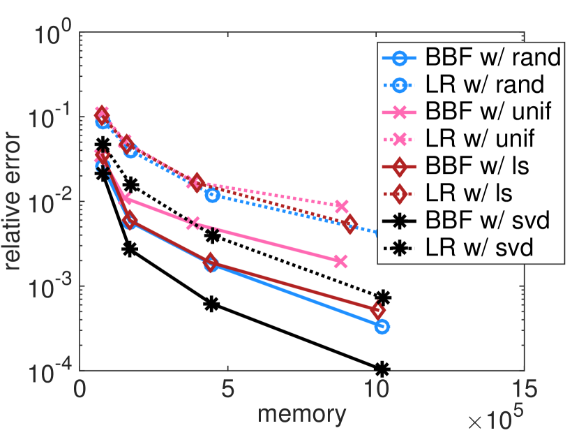
(a) Abalone, $h$=2

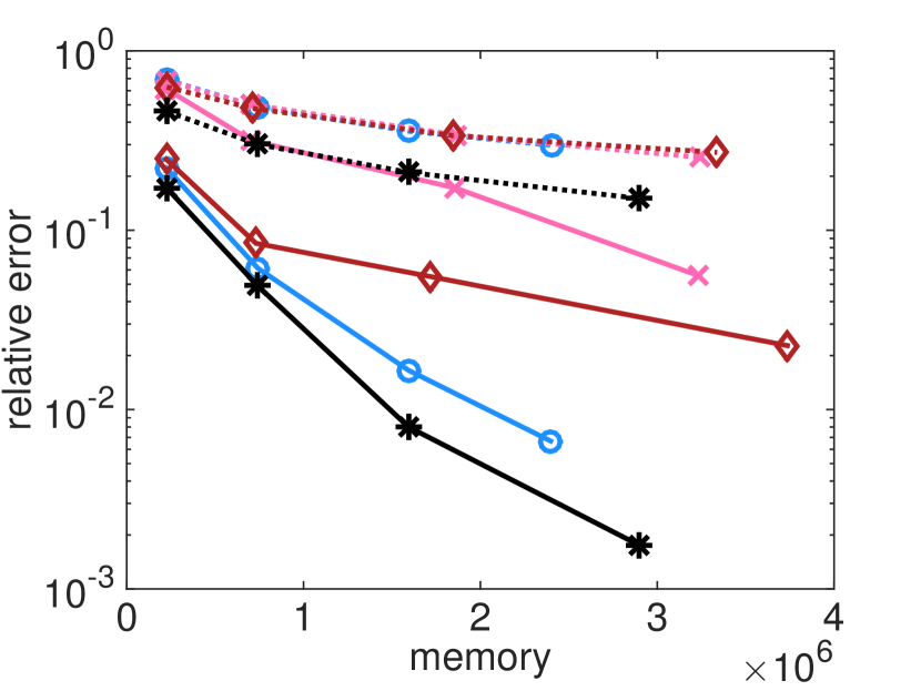
(b) Pendigits, $h$ = 2

Figure 13: Kernel approximation error versus memory cost for BBF and low-rank structure with different sampling methods. Gaussian kernel is used. The results are averaged over 5 runs. BBF (solid lines) uses the structure described in Figure 8, and LR (dash lines) uses a low-rank structure. “rand”: randomized sampling; “unif”: uniform sampling; “ls”: leverage score sampling; “svd”: an SVD is used for computing the basis.

4.2 BBF algorithm

In this section, we experimentally evaluate the performance of our BBF algorithm with other state-of-art kernel approximation methods. subsubsection 4.2.1 and subsubsection 4.2.2 examine the matrix reconstruction error under varying memory budget and kernel bandwidth parameters. subsubsection 4.2.3 applies the approximations to the kernel ridge regression problem. Finally, subsubsection 4.2.4 compares the linear complexity of BBF with the IFGT [41]. Throughout the experiments, we use BBF to denote our algorithm, whose input parameters are computed from our pre-computation algorithm.

In what follows, we briefly introduce some implementation and input parameter details for the methods we are comparing to.

• The naïve Nyström (Nys). We uniformly sampled $2k$ columns without replacement for a rank $k$ approximation.

• $k$-means Nyström (kNys). It uses $k$-means clustering and sets the centroids to be the landmark points. We used the code provided by the author.

• Leverage score Nyström (lsNys). It samples columns with probabilities proportional to the statistical leverage scores. We calculated the approximated leverage scores [14] and sampled $2k$ columns with replacement for a rank-$k$ approximation.

• Memory Efficient Kernel Approximation (MEKA). We used the code provided by the author.

• Random Kitchen Sinks (RKS). We used our own MATLAB implementation based on their algorithm.

• Improved Fast Gauss Transform (IFGT). We used the C++ code provided by the author.

4.2.1 Approximation with varying memory budget

We consider the reconstruction errors from different methods when the memory cost varies. The memory cost (storage) is also a close approximation of the running time for a matrix-vector multiplication. In addition, computing memory is more accurate than running time, which is sensitive to the implementation and algorithmic details. In our experiments, we indirectly increased the memory cost by requesting a lower tolerance in BBF. The memories for all the methods were fixed to be roughly the same in the following way. For low rank methods, the input rank was set to be the memory of BBF divided by the matrix size. For MEKA, the input number of clusters was set to be the same as BBF; the “eta” parameter (the percentage of blocks to be set to zeros) was also set to be similar as BBF.

Figure 14 and Figure 15 show the reconstruction error versus memory cost on real datasets and 2D synthetic datasets, respectively. We see that BBF achieves comparable and often significantly lower error than the competing methods regardless of the memory cost. There are two observations worth noting. First, the BBF outperforms the exact SVD which is the best rank-$r$ approximation, and it outperforms with a factorization complexity that is only linear rather than cubic. This has demonstrated the superiority of the BBF structure over the low-rank structure. Second, even when compared to a similar structure as MEKA, BBF achieves a lower error whose variance is also smaller, and it achieves so with a similar factorization complexity. These have verified that the representation of BBF is more accurate and the constructing algorithm is more stable.

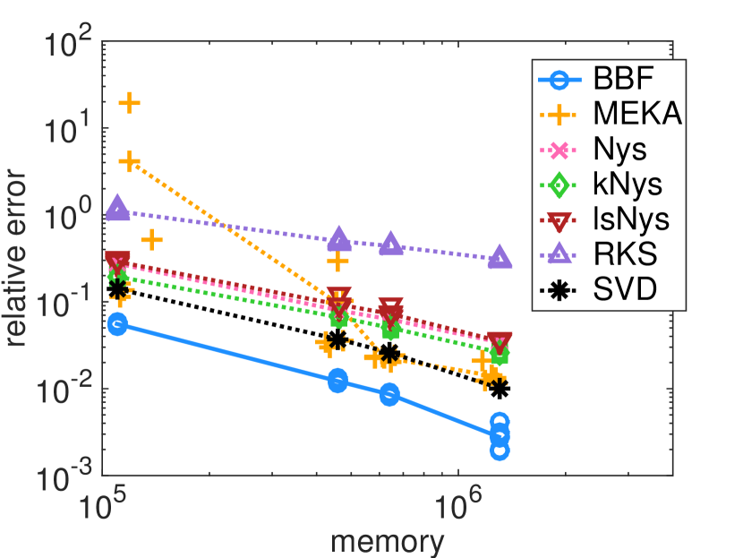
(a) Abalone, $h$ = 1

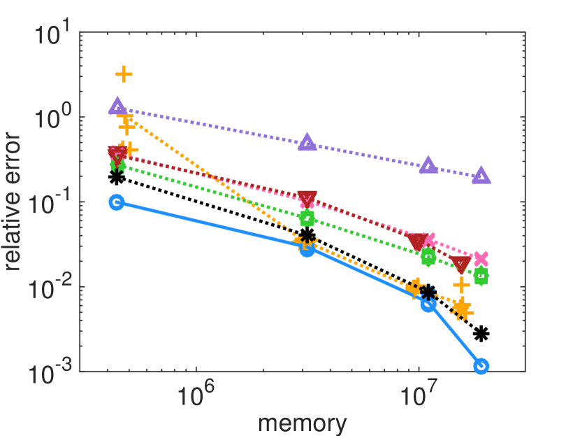
(b) Pendigits, $h$ = 2

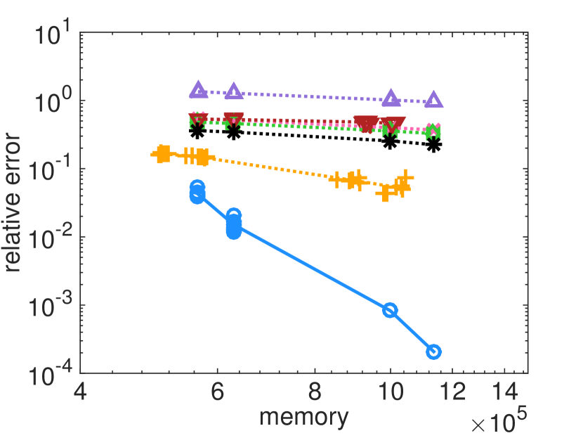
(c) CTG, $h=0.5$

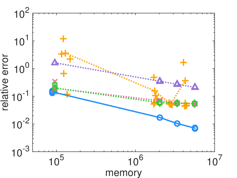
(d) EMG, $h=0.1$

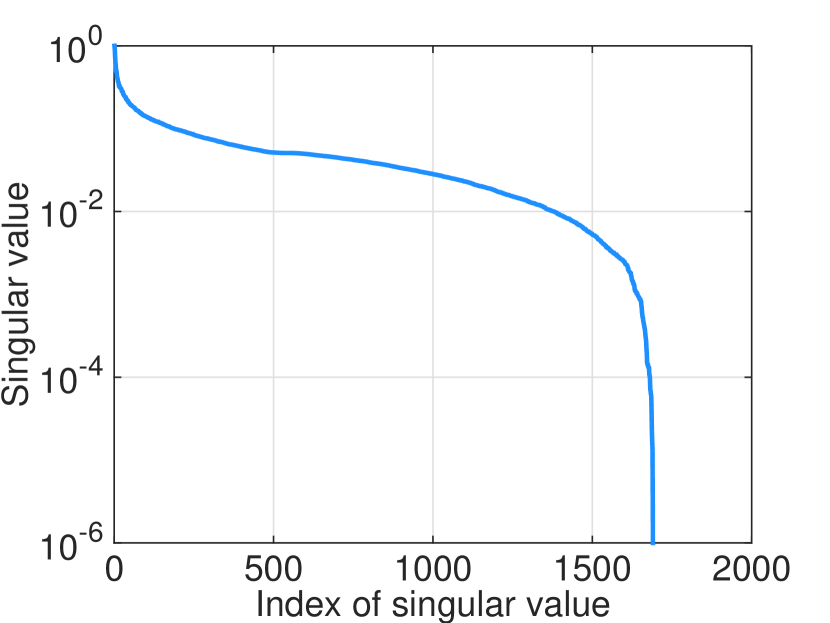
(e) Singular values (CTG)

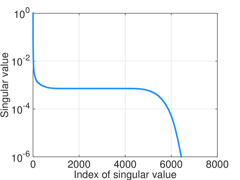
(f) Singular values (EMG)

Figure 14: Comparisons of BBF (our algorithm) with competing methods. Top four plots (loglog scale) share the same legend. For each method, we show the improvement in error as more memory is available. For each memory footprint, we report the error of 5 runs of each algorithm. Each run is shown with a marker, while the lines represent the average error. For CTG and EMG datasets, the parameter $h$ was chosen to achieve higher $F_{1}$ score on smaller classes, which leads to matrices with higher ranks as shown by the plateau or slow decay of singular values in the bottom plots subplots (e) and (f).

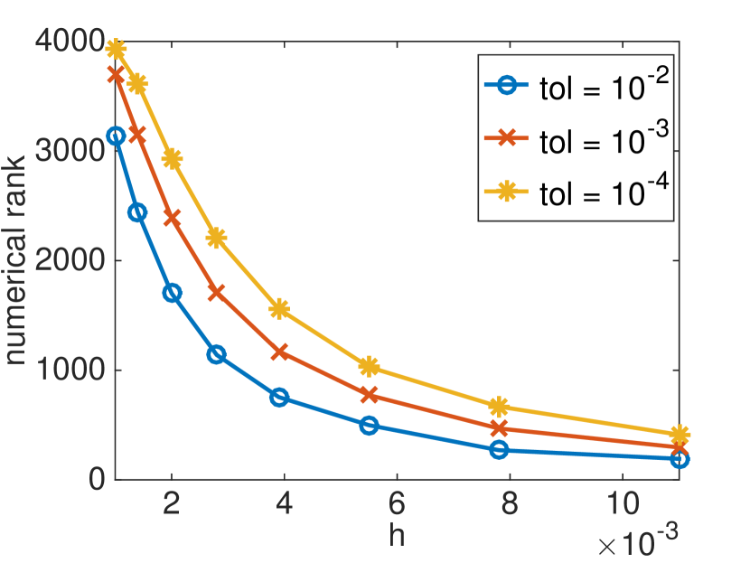
(a) Numerical ranks of the kernel matrix

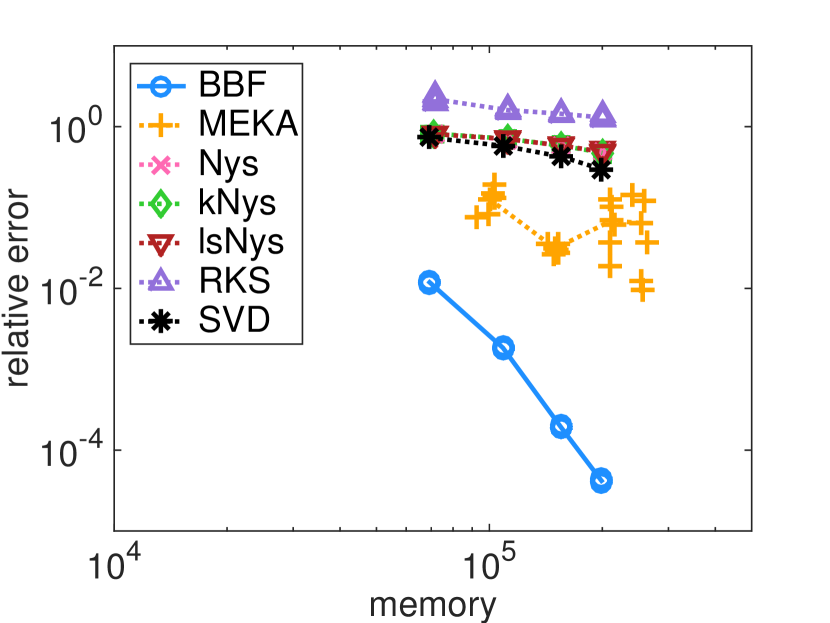
(b) Relative error versus memory cost

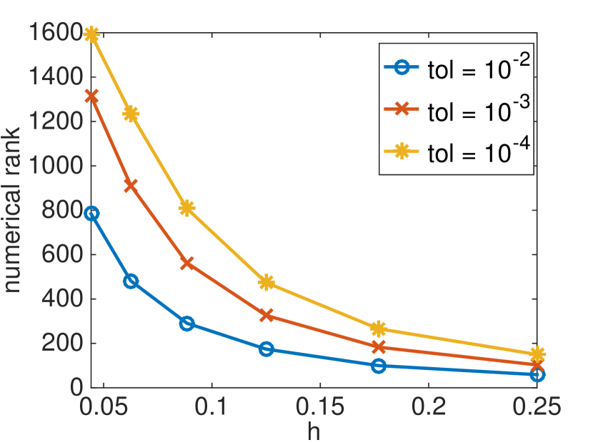
(c) Numerical ranks of the kernel matrix

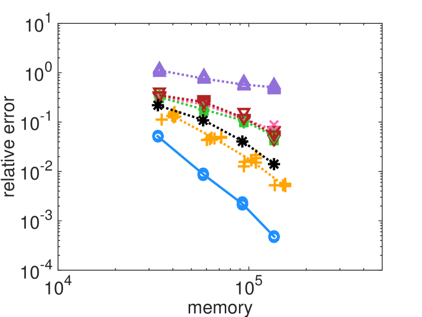
(d) Relative error versus memory cost

Figure 15: The left plots report the numerical ranks of matrices versus $h$ and the right plots report the relative error versus memory. The data for top plots has alternating labels (see Figure 5 with 100 clusters) while the data for the bottom plots has smaller clusters surrounded by larger ones (see Figure 6). The values of $h$ reported in subplot $(a)$ and $(c)$ yield test accuracy greater than 0.99. The $h$ in $(b)$ and $(d)$ are the largest optimal $h$ with value 0.0127 and 0.25 respectively. For each memory cost, we report the relative error of 5 runs of each algorithm. The number of clusters for BBF was fixed at 20 for subplot $(b)$ and selected automatically for subplot $(d)$.

4.2.2 Approximation with varying kernel bandwidth parameters

We consider the reconstruction errors with varying decay patterns of singular values, which we achieve by choosing a wide range of kernel bandwidth parameters. The memory for all methods are fixed to be roughly the same.

The plots on the left of Figure 16 show the average matrix reconstruction error versus $1/h^{2}$. We see that for all the low-rank methods, the error increases when $h$ decreases. When $h$ becomes smaller, the kernel function becomes less smooth, and consequently the matrix rank increases. This relation between $h$ and the matrix rank are revealed in some statistics listed in Table 4. The results in the table are consistent with the results shown in [18] for varying kernel bandwidth parameters.

Table 4: Summary statistics for abalone and pendigits datasets with the Gaussian kernel, where $r$ is the rank, $M$ is the exact matrix, and $M_{r}$ is the best rank-$r$ approximation for $M$. $\Big{\lceil}\frac{\|M\|_{F}^{2}}{\|M\|_{2}^{2}}\Big{\rceil}$ is referred to as the stable rank and is an underestimate of the rank. $l_{r}$ represents the $r$-th largest leverage score scaled by $\tfrac{n}{r}$.

Abalone ($r$ = 100)				Pendigits ($r$ = 252)
$\frac{1}{h^{2}}$	$\Big{\lceil}\frac{\|M\|_{F}^{2}}{\|M\|_{2}^{2}}\Big{\rceil}$	$100\frac{\|M_{r}\|_{F}}{\|M\|_{F}}$	$l_{r}$	$\frac{1}{h^{2}}$	$\Big{\lceil}\frac{\|M\|_{F}^{2}}{\|M\|_{2}^{2}}\Big{\rceil}$	$100\frac{\|M_{r}\|_{F}}{\|M\|_{F}}$	$l_{r}$
0.25	2	99.99	4.34	0.1	3	99.99	2.39
1	4	99.86	2.03	0.25	6	99.79	1.83
4	5	97.33	1.94	0.44	8	98.98	1.72
25	15	72.00	5.20	1	12	93.64	2.02
100	175	33.40	12.60	2	33	77.63	2.90
400	931	19.47	20.66	4	207	49.60	4.86
1000	1155	16.52	20.88	25	2794	19.85	14.78

In the large-$h$ regime, the gap in error between BBF and other methods is small. In such regime, the matrix is low rank, and the low-rank algorithms work effectively. Hence, the difference in error is not significant. In the small-$h$ regime, the gap starts to increase. In this regime, the matrix becomes close to diagonal dominant, and the low-rank structure, as a global structure, cannot efficiently capture the information along the diagonal; while for BBF, the pre-computation procedure will increase the number of clusters to better approximate the diagonal part, and the off-diagonal blocks can be set to 0 due to their small entries. By efficiently using the memory, BBF is favorable in all cases, from low-rank to nearly diagonal.

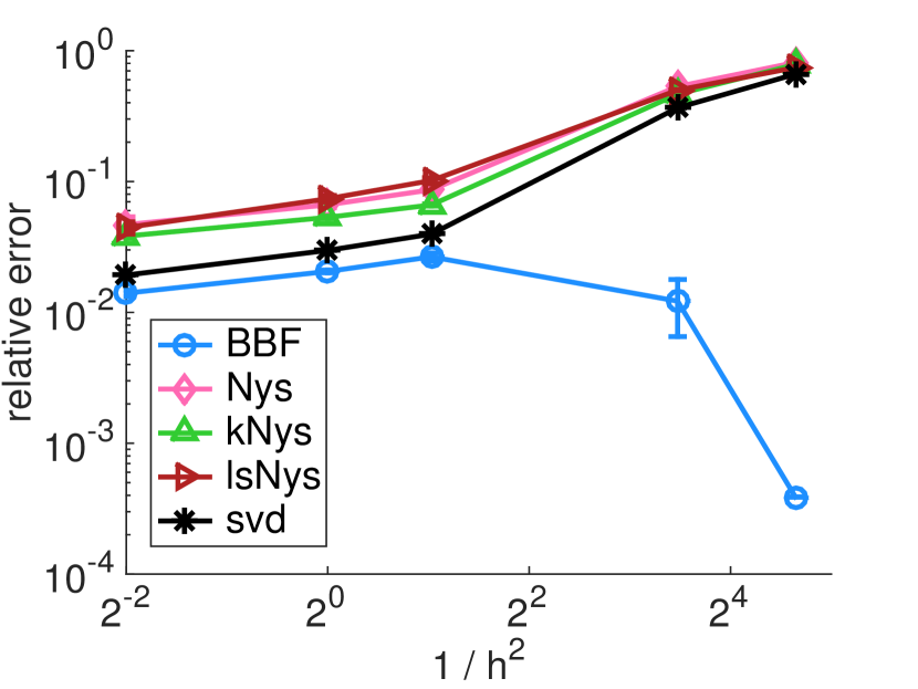
(a) Abalone

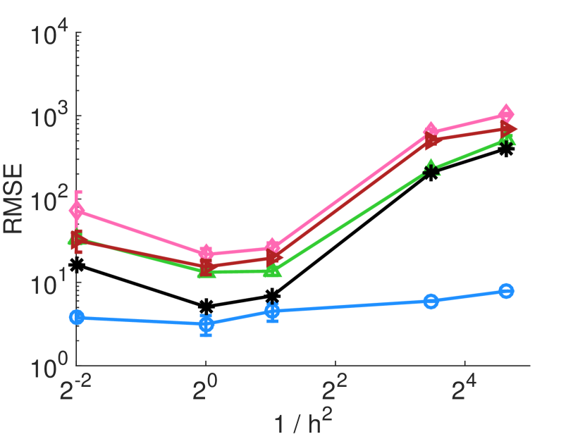
(b) Abalone

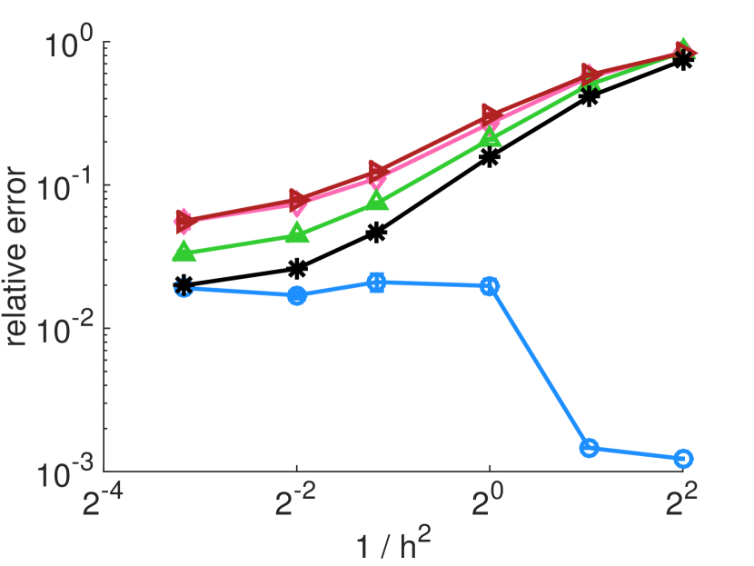
(c) Pendigits

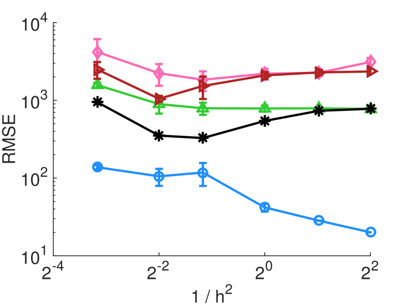
(d) Pendigits

Figure 16: Plots for relative error vers $1/h^{2}$ for different kernel approximation methods. The memory costs for all methods and all kernel parameters are fixed to be roughly the same. The kernel function used is the Gaussian kernel. As the rank of the matrix increases ($h$ decreases), the gap in error between low-rank approximation methods and BBF increases.

4.2.3 Kernel ridge regression

We consider the kernel ridge regression. The standard optimization problem for the kernel ridge regression is

(4) $$\min_{{\bm{\alpha}}}\|K{\bm{\alpha}}-{\bf y}\|^{2}+\lambda\|{\bm{\alpha}}\|^{2},$$

where $K$ is a kernel matrix, ${\bf y}$ is the target, and $\lambda>0$ is the regularization parameter. The minimizer is given by the solution of the following linear system

(5) $$(K+\lambda I){\bm{\alpha}}={\bf y}.$$

The linear system can be solved by an iterative solver, e.g. MINRES [33], and the complexity is $O(n^{2}T)$ where $n^{2}$ is from matrix-vector multiplications and $T$ denotes the iteration number. If we can approximate $K$ by $\widehat{K}$ which can be represented in lower memory, then the solving time can be accelerated. This is because the memory is a close approximation for the running time of a matrix-vector multiplication. We could also solve the approximated system directly when the matrix can be well-approximately by a low-rank matrix, that is, we compute the inversion of $\widehat{K}$ first by the Woodbury formula and then apply the inversion to ${\bf y}$.

In the experiments, we approximated $K$ by $\widehat{K}$, and solved the following approximated system with MINRES.

(6) $$(\widehat{K}+\lambda I){\bm{\alpha}}={\bf y}.$$

The dataset was randomly divided into training set (80%) and testing set (20%). The kernel used is the Laplacian kernel $K({\bf x},{\bf y})=\exp(\|{\bf x}-{\bf y}\|/h)$ for this subsection. We report the test root-mean-square error (RMSE) which is defined as

(7) $$\sqrt{\frac{1}{n_{\text{test}}}\|K_{\text{test}}\hat{\bm{\alpha}}-{\bf y}_{\text{test}}\|_{F}^{2}},$$

where $K_{\text{test}}$ is the interaction matrix between the test data and training data, $\hat{\bm{\alpha}}$ is the solution from solving Equation 6, and ${\bf y}_{\text{test}}$ is the true test target. Figure 17 shows the test RMSE with varying memory cost of the approximation. We see that with the same memory footprint, the BBF achieves lower test error.

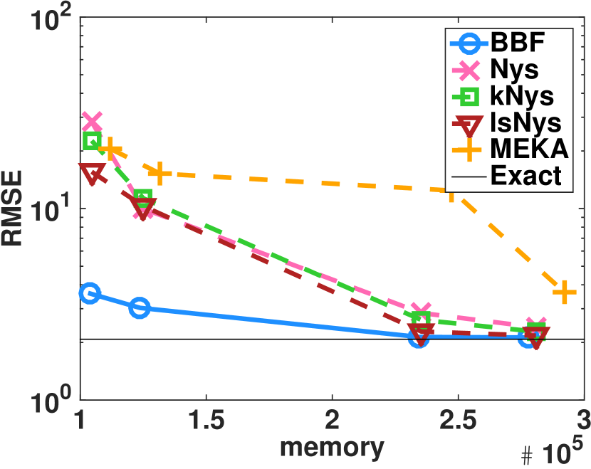
(a) Abalone, (4, $2^{-4}$)

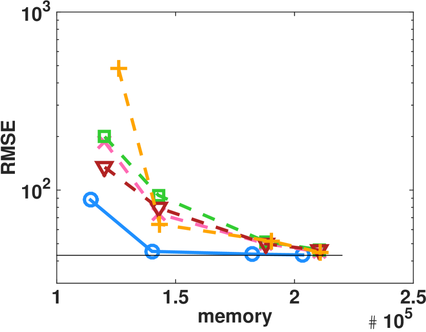
(b) Pendigits, (22.6, $2^{-5}$)

(c) Cpusmall, (4.94, $2^{-5}$)

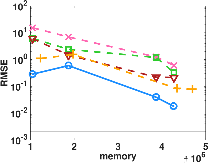
(d) Mushroom, (4.63, $2^{-5}$)

Figure 17: Test RMSE versus memory for kernel ridge regression. For each memory cost, we report the results averaged over 5 runs. The black line on the bottom of each plot represents the test RMSE when using the exact matrix. The kernel parameter $h$ and the regularization parameter $\lambda$ were selected by a 5-fold cross-validation with a grid search, and the selected $(h,\lambda)$ pairs are listed in the subcaption.

Discussion. For downstream prediction tasks, better generalization error could be achieved by using the surrogate kernel, which is the kernel matrix between the testing points and landmark points, instead of the exact kernel matrix for naïve Nyström, $k$-means Nyström, leverage score Nyström, and random kitchen sink. Based on our experience, using surrogate kernels with Nyström methods and random Fourier methods achieves competitive testing accuracy as that of BBF. Hence, although BBF significantly outperforms Nyström methods and random Fourier methods in the approximation of kernel matrices, the advantage of BBF in prediction compared with surrogate kernels is less pronounced.

Meanwhile, an easy modification of BBF can be used to construct a surrogate kernel for downstream predictions as well. Specifically, for $U_{i}$, we can set $U_{i}$ as the carefully sampled important columns with points denoted as $X_{i}$, instead of the column basis of those sampled columns. This further reduces our factorization cost due to the removal of the orthonormalization step. Once these important columns are available, the middle matrix $C$ can be constructed identical to that in Algorithm 5. These steps construct the modified BBF, which can be used to accelerate the linear system solve of (6) and obtain ${\bm{\alpha}}$ efficiently. Then, the coefficient for the surrogate kernel is computed as $\widetilde{{\bm{\alpha}}}=CU^{\dagger}{\bm{\alpha}}$. We denote $\widetilde{{\bm{\alpha}}}_{i}$ as the coefficient for cluster $i$. The downstream prediction task, then, is divided into two steps. First, for a testing point ${\bf x}_{test}$, we find the cluster $i$ that ${\bf x}_{test}$ belongs to. Second, we compute the predictions $y_{test}$ as $K({\bf x}_{test},X_{i})\widetilde{{\bm{\alpha}}_{i}}$.

With this modified BBF and the corresponding prediction procedure, assuming a surrogate kernel of the same size is used, it will be more efficient to compute the coefficients of the surrogate kernel as well as the predictions through BBF than Nyström methods or random Fourier methods.

4.2.4 Comparison with the improved fast gauss transform (IFGT)

We benchmarked the linear complexity of the Improved Fast Gauss Transform (IFGT) [41] and BBF. IFGT was proposed to alleviate the dimensionality issue for the Gaussian kernel. For a fixed dimension $d$, the IFGT has a linear complexity in terms of application time and memory cost; regrettably, when $d$ increases (e.g., $d\geq 10$) the algorithm requires a large number of data points $n$ to make this linear behavior visible. BBF, on the other hand, does not require a large $n$ to observe a linear growth.

We verify the influence of dimension $d$ on the complexity of BBF and the IFGT on synthetic datasets. We fixed the tolerance to be $10^{-3}$ throughout the experiments. Figure 18 shows the time versus the number of points. We focus only on the trend of time instead of the absolute value, because the IFGT was implemented in C++ while BBF was in MATLAB. We see that the growth rate of IFGT is linear when $d=5$ but falls back to quadratic when $d=40$; the growth rate of BBF, however, remains linear.

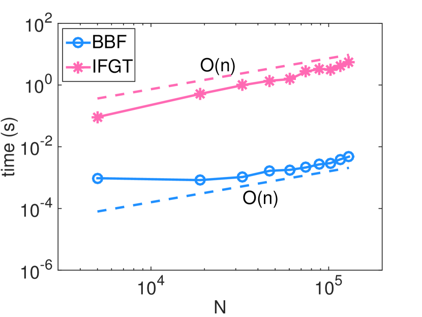
(a) Application time (d = 5)

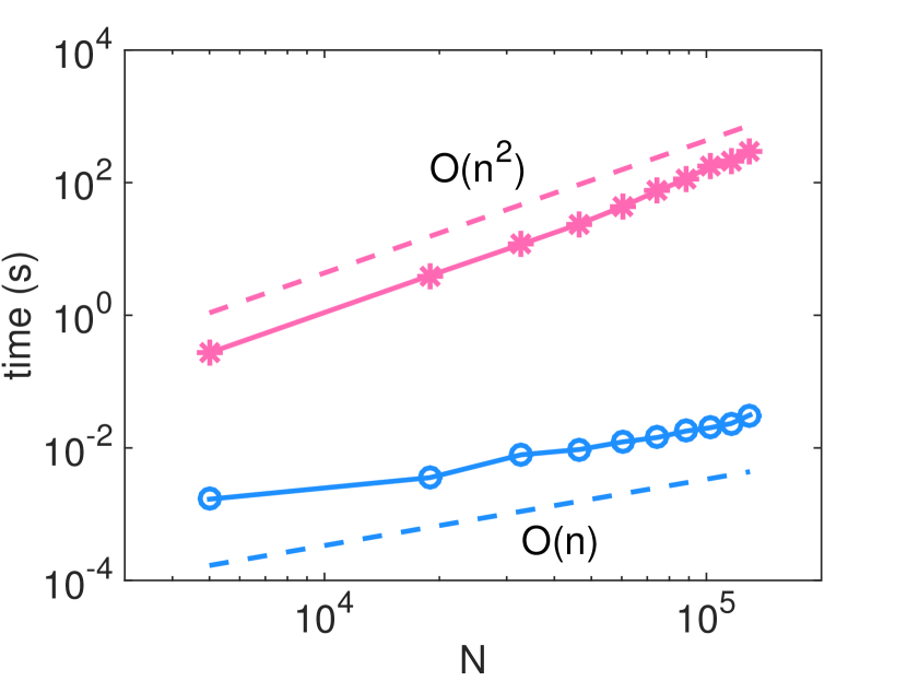
(b) Application time (d = 40)

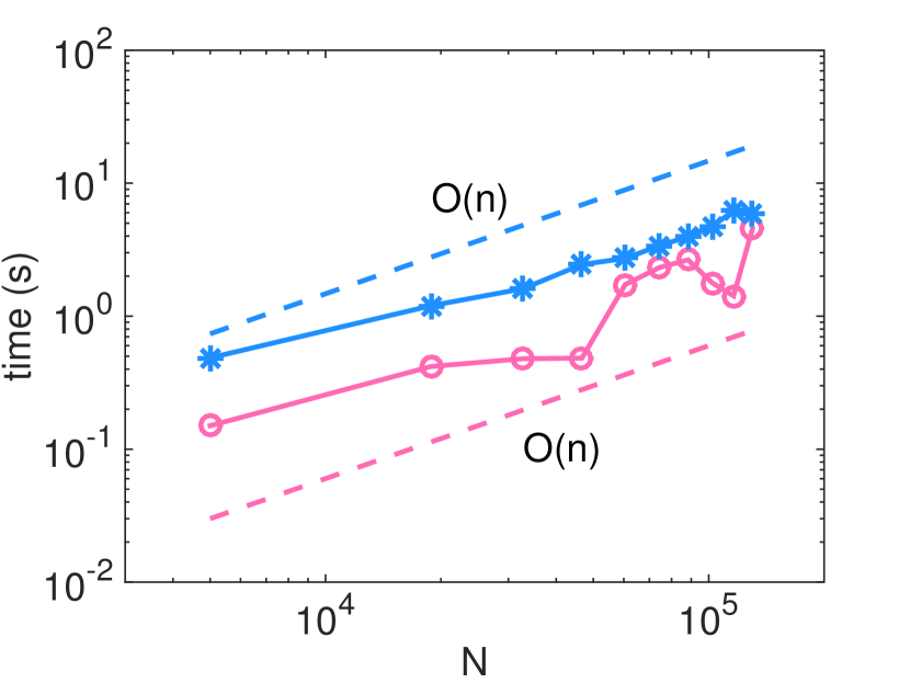
(c) Total time (d = 5)

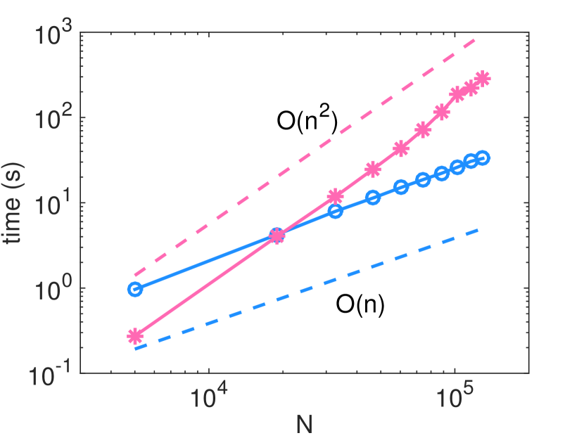
(d) Total time (d = 40)

Figure 18: Timing (loglog scale) for IFGT and BBF on a synthetic dataset with dimension $d=5$ and $40$. We generated 10 centers uniformly at random in a unit cube, and around each center we randomly generated data with standard deviation 0.1 along each dimension. The tolerance and the kernel parameter $h$ were set to $10^{-3}$, and 0.5, respectively. All the plots share the same legends. The top plots show the application time (matrix-vector product), and bottom plots show the total time (factorization and application). The timing for BBF is linear for all dimensions, while the timing for the IFGT falls back to quadratic when $d$ increases.

5 Conclusions and future work

In this paper, we observed that for classification datasets whose decision boundaries are complex, i.e., of small radius of curvature, a small bandwidth parameter is needed for a high prediction accuracy. In practical datasets, this complex decision boundary occurs frequently when there exist a large variability in class sizes or radii. These small bandwidths result in kernel matrices whose ranks are not low and hence traditional low-rank methods are no longer efficient. Moreover, for many machine-learning applications, low-rank approximations of dense kernel matrices are inefficient. Hence, we are interested in extending the domain of availability of low-rank methods and retain computational efficiency. Specifically, we proposed a structured low-rank based algorithm that is of linear memory cost and floating point operations, that remains accurate even when the kernel bandwidth parameter is small, i.e., when the matrix rank is not low. We experimentally demonstrated that the algorithm works in fact for a wide range of kernel parameters. Our algorithm achieves comparable and often orders of magnitude higher accuracy than other state-of-art kernel approximation methods, with the same memory cost. It also produces errors with smaller variance, thanks to the sophisticated randomized algorithm. This is in contrast with other randomized methods whose error fluctuates much more significantly. Applying our algorithm to the kernel ridge regression also demonstrates that our method competes favorably with the state-of-art approximation methods.

There are a couple of future directions. One direction is on the efficiency and performance of the downstream inference tasks. The focus of this paper is on the approximation of the kernel matrix itself. Although the experimental results have demonstrated good performances in real-world regression tasks, we could further improve the downstream tasks by relaxing the orthogonality constrains of the $U_{i}$ matrices. That is, we can generate $U_{i}$ from interpolative decomposition [11], which allows us to share the same advantages as algorithms using Nys and RKS. Another direction is on the evaluation metric for the kernel matrix approximation. This paper used the conventional Frobenius norm to measure the approximation performance. Zhang et al. [43] proposed a new metric that better measures the downstream performance. The new metric suggests that to achieve a good generalization performance, it is important to have a high-rank approximation. This suggestion aligns well with the design of BBF and further emphasizes its advantage. Evaluating BBF under the new metric will be explored in the future. Last but not least, the BBF construction did not consider the regularization parameter used in many learning algorithms. We believe that the regularization parameter could facilitate the low-rank compression of the kernel matrix in our BBF, while the strategy requires further exploration.

References

- [1] A. E. Alaoui and M. W. Mahoney, Fast randomized kernel ridge regression with statistical guarantees, in Proceedings of the 28th International Conference on Neural Information Processing Systems - Volume 1, NIPS’15, Cambridge, MA, USA, 2015, MIT Press, pp. 775–783.
- [2] P. Amestoy, C. Ashcraft, O. Boiteau, A. Buttari, J. L’Excellent, and C. Weisbecker, Improving multifrontal methods by means of block low-rank representations, SIAM Journal on Scientific Computing, 37 (2015), pp. A1451–A1474.
- [3] P. Amestoy, C. Ashcraft, O. Boiteau, A. Buttari, J.-Y. L’Excellent, and C. Weisbecker, Improving multifrontal methods by means of block low-rank representations, SIAM Journal on Scientific Computing, 37 (2015), pp. A1451–A1474.
- [4] A. Aminfar, S. Ambikasaran, and E. Darve, A fast block low-rank dense solver with applications to finite-element matrices, Journal of Computational Physics, 304 (2016), pp. 170–188.
- [5] F. Bach, Sharp analysis of low-rank kernel matrix approximations, in Proceedings of the 26th Annual Conference on Learning Theory, 2013, pp. 185–209.
- [6] K. Bache and M. Lichman, UCI machine learning repository, 2013.
- [7] J. Bouvrie and B. Hamzi, Kernel methods for the approximation of nonlinear systems, SIAM Journal on Control and Optimization, 55 (2017), pp. 2460–2492.
- [8] S. Chandrasekaran, M. Gu, and T. Pals, A fast ULV decomposition solver for hierarchically semiseparable representations, SIAM Journal on Matrix Analysis and Applications, 28 (2006), pp. 603–622.
- [9] C.-C. Chang and C.-J. Lin, LIBSVM: A library for support vector machines, ACM Transactions on Intelligent Systems and Technology, 2 (2011), pp. 27:1–27:27. Software available at http://www.csie.ntu.edu.tw/~cjlin/libsvm.
- [10] J. Chen, H. Avron, and V. Sindhwani, Hierarchically compositional kernels for scalable nonparametric learning, J. Mach. Learn. Res., 18 (2017), p. 2214–2255.
- [11] H. Cheng, Z. Gimbutas, P.-G. Martinsson, and V. Rokhlin, On the compression of low rank matrices, SIAM J. Sci. Comput., 26 (2005), pp. 1389–1404.
- [12] E. Darve, The fast multipole method I: error analysis and asymptotic complexity, SIAM Journal on Numerical Analysis, 38 (2000), pp. 98–128.
- [13] , The fast multipole method: numerical implementation, Journal of Computational Physics, 160 (2000), pp. 195–240.
- [14] P. Drineas, M. Magdon-Ismail, M. W. Mahoney, and D. P. Woodruff, Fast approximation of matrix coherence and statistical leverage, The Journal of Machine Learning Research, 13 (2012), pp. 3475–3506.
- [15] P. Drineas and M. W. Mahoney, On the Nyström method for approximating a gram matrix for improved kernel-based learning, The Journal of Machine Learning Research, 6 (2005), pp. 2153–2175.
- [16] B. Engquist, L. Ying, et al., A fast directional algorithm for high frequency acoustic scattering in two dimensions, Communications in Mathematical Sciences, 7 (2009), pp. 327–345.
- [17] W. Fong and E. Darve, The black-box fast multipole method, Journal of Computational Physics, 228 (2009), pp. 8712–8725.
- [18] A. Gittens and M. W. Mahoney, Revisiting the Nyström method for improved large-scale machine learning, The Journal of Machine Learning Research, 17 (2016), pp. 3977–4041.
- [19] G. H. Golub and C. F. Van Loan, Matrix computations, vol. 3, JHU Press, 2012.
- [20] L. Greengard and V. Rokhlin, A fast algorithm for particle simulations, Journal of computational physics, 73 (1987), pp. 325–348.
- [21] , A new version of the fast multipole method for the Laplace equation in three dimensions, Acta numerica, 6 (1997), pp. 229–269.
- [22] L. Greengard and J. Strain, The fast gauss transform, SIAM Journal on Scientific and Statistical Computing, 12 (1991), pp. 79–94.
- [23] M. Gu and S. C. Eisenstat, Efficient algorithms for computing a strong rank-revealing QR factorization, SIAM Journal on Scientific Computing, 17 (1996), pp. 848–869.
- [24] W. Hackbusch, A sparse matrix arithmetic based on -matrices. Part I: Introduction to -matrices, Computing, 62 (1999), pp. 89–108.
- [25] W. Hackbusch and S. Börm, Data-sparse approximation by adaptive matrices, Computing, 69 (2002), pp. 1–35.
- [26] W. Hackbusch and B. N. Khoromskij, A sparse -matrix arithmetic., Computing, 64 (2000), pp. 21–47.
- [27] N. Halko, P.-G. Martinsson, and J. A. Tropp, Finding structure with randomness: Probabilistic algorithms for constructing approximate matrix decompositions, SIAM review, 53 (2011), pp. 217–288.
- [28] M. R. Hestenes and E. Stiefel, Methods of conjugate gradients for solving linear systems, vol. 49, NBS Washington, DC, 1952.
- [29] Y. Li, H. Yang, E. R. Martin, K. L. Ho, and L. Ying, Butterfly factorization, Multiscale Modeling & Simulation, 13 (2015), pp. 714–732.
- [30] Y. Li, H. Yang, and L. Ying, Multidimensional butterfly factorization, Applied and Computational Harmonic Analysis, 44 (2018), pp. 737 – 758.
- [31] E. Liberty, F. Woolfe, P.-G. Martinsson, V. Rokhlin, and M. Tygert, Randomized algorithms for the low-rank approximation of matrices, Proceedings of the National Academy of Sciences, 104 (2007), pp. 20167–20172.
- [32] M. W. Mahoney, Randomized algorithms for matrices and data, Foundations and Trends in Machine Learning, 3 (2011), pp. 123–224.
- [33] C. C. Paige and M. A. Saunders, Solution of sparse indefinite systems of linear equations, SIAM Journal on Numerical Analysis, 12 (1975), pp. 617–629.
- [34] T. Sarlos, Improved approximation algorithms for large matrices via random projections, in Foundations of Computer Science, 2006. FOCS’06. 47th Annual IEEE Symposium on, IEEE, 2006, pp. 143–152.
- [35] B. Savas, I. S. Dhillon, et al., Clustered low rank approximation of graphs in information science applications., in SDM, SIAM, 2011, pp. 164–175.
- [36] S. Si, C.-J. Hsieh, and I. Dhillon, Memory efficient kernel approximation, in Proceedings of The 31st International Conference on Machine Learning, 2014, pp. 701–709.
- [37] M. L. Stein, Limitations on low rank approximations for covariance matrices of spatial data, Spatial Statistics, 8 (2014), pp. 1 – 19.
- [38] M. L. Stein, Limitations on low rank approximations for covariance matrices of spatial data, Spatial Statistics, 8 (2014), pp. 1–19.
- [39] R. Wang, Y. Li, and E. Darve, On the numerical rank of radial basis function kernels in high dimensions, SIAM J. Matrix Anal. Appl., 39 (2018), pp. 1810–1835.
- [40] J. Xia, S. Chandrasekaran, M. Gu, and X. S. Li, Fast algorithms for hierarchically semiseparable matrices, Numerical Linear Algebra with Applications, 17 (2010), pp. 953–976.
- [41] C. Yang, R. Duraiswami, N. A. Gumerov, and L. Davis, Improved fast Gauss transform and efficient kernel density estimation, in Computer Vision, 2003. Proceedings. Ninth IEEE International Conference on, IEEE, 2003, pp. 664–671.
- [42] L. Ying, G. Biros, and D. Zorin, A kernel-independent adaptive fast multipole algorithm in two and three dimensions, Journal of Computational Physics, 196 (2004), pp. 591–626.
- [43] J. Zhang, A. May, T. Dao, and C. Ré, Low-precision random fourier features for memory-constrained kernel approximation, mar 2019.
- [44] K. Zhang and J. T. Kwok, Clustered Nyström method for large scale manifold learning and dimension reduction, Neural Networks, IEEE Transactions on, 21 (2010), pp. 1576–1587.