A New Selection Operator for the Discrete Empirical Interpolation Method – improved a priori error bound and extensions
Abstract
This paper introduces a new framework for constructing the Discrete Empirical Interpolation Method (DEIM) projection operator. The interpolation node selection procedure is formulated using the QR factorization with column pivoting, and it enjoys a sharper error bound for the DEIM projection error. Furthermore, for a subspace given as the range of an orthonormal , the DEIM projection does not change if is replaced by with arbitrary unitary matrix . In a large-scale setting, the new approach allows modifications that use only randomly sampled rows of , but with the potential of producing good approximations with corresponding probabilistic error bounds. Another salient feature of the new framework is that robust and efficient software implementation is easily developed, based on readily available high performance linear algebra packages.
keywords:
empirical interpolation, nonlinear model reduction, proper orthogonal decomposition, projections, QR factorization, randomized sampling, rank revealing factorizationAMS:
15A12, 15A23, 65F35, 65M20, 65M22, 93B40, 93C151 Introduction
Direct numerical simulation of dynamical systems plays a crucial role in studying a great variety of complex physical phenomena in areas ranging from neuron modeling to microchip design. The ever-increasing demand for accuracy leads to dynamical systems of ever-larger scale and complexity. Simulation in such large-scale settings can make overwhelming demands on computational resources; thus creating a need for model reduction to create smaller, faster approximations to complex dynamical systems that still guarantee high fidelity.
1.1 Model Reduction by Galerkin Projection
Consider the following nonlinear dynamical system of ordinary differential equations (ODE)
| (1) |
where , , and . In (1), is the state and is the external forcing term (input); thus (1) has degrees of freedom and inputs.
Systems of the form (1) with very large state-space dimension ( or higher) arise in many disciplines and typically originate from discretization of partial differential equation models. The goal of model reduction is to replace (1) with a reduced surrogate dynamical system having much lower state space dimension, . The reduced model will then have the structure
| (2) |
where , , and .
We will use a Galerkin projection to construct the reduced model (2): Let be an -dimensional subspace spanned by the columns of . Then, we approximate the full-state using the ansatz and enforce the Galerkin orthogonality condition to obtain the reduced model (2) with the reduced model quantities given by
| (3) |
1.2 Galerkin Projection using Proper Orthogonal Decomposition
For linear dynamical systems, i.e., when in (1), a plethora of methods exist to perform model reduction: These include gramian based methods such as Balanced Truncation [37, 36] and Optimal Hankel Norm Approximation [24] or rational interpolation based methods such Iterative Rational Krylov Algorithm [27]. These methods rely on the concept of transfer function and perform model reduction independent of the input . These ideas have been recently extended to systems with bilinear [4, 6, 23] and quadratic nonlinearities [26, 7]. For general nonlinearities, Proper Orthogonal Decomposition (POD) is the most-commonly used method. POD [35, 9] obtains the model reduction basis from a truncated SVD approximation to a matrix of “snapshots”, a numerically computed trajectory of the full model. It is related to methods (and known by other names) such as Principal Component Analysis (PCA) in statistical analysis [29] and Karhunen-Loéve expansion [34] in stochastic analysis.
To construct the model reduction basis via POD, one performs a numerical simulation of (1) for an input and initial condition . Let denote the snapshots resulting from this numerical simulation; i.e, for . Construct the POD snapshot matrix
| (4) |
and compute its thin SVD
| (5) |
where , , and with , and , with . Then model reduction by POD chooses as the leading left singular vectors of corresponding to the largest singular values. Using MATLAB notation, this corresponds to . This basis selection by POD minimizes over all with orthonormal columns. Since the objective function does not change if is post-multiplied by an arbitrary orthogonal matrix, this procedure actually seeks an –dimensional subspace that optimally captures the snapshots in the least squares sense. For more details on POD, we refer the reader to [28, 32].
1.3 The lifting bottleneck
Even though the state of the reduced model (2) lives in an -dimensional subspace, definition of the reduced nonlinear term in (3) requires lifting back to the full -dimensional subspace in order to evaluate the nonlinear term; this is known as the lifting bottleneck and degrades the performance of reduced models for nonlinear systems. Various approaches exist to tackle this issue; see, e.g., [21, 5, 3, 39, 14]. In this paper, we focus on the Discrete Empirical Interpolation Method (DEIM) [39], a discrete variant of the Empirical Interpolation Method introduced in [5].
As explained in the original source [39], DEIM can be used to approximate and efficiently evaluate a general nonlinear function , which is not necessarily tied to the model reduction set-up we discussed above. For example, could be a vector-valued function of possibly multidimensional parameter . Therefore, following [39], we will present the DEIM construction and our analysis for a generic nonlinear vector valued function , yet will point out the implications for nonlinear model reduction.
1.4 DEIM
Given a nonlinear function with and a matrix of rank , DEIM approximation of is defined by [39, Definition 3.1]
| (6) |
where is matrix obtained by selecting certain columns of the identity matrix . With the DEIM approximation to defined as in (6), the nonlinear term in the reduced model (2) is now approximated by
| (7) |
An effective numerical implementation of is different than its analytical formula in (7) and allows computing without lifting to the full dimension and by only selecting a certain rows of . We skip those details and refer the reader to [39, §3.4].
Computation of the DEIM basis
In an application, the matrix can be computed as follows. For a finite grid , the function is sampled at and, as done for state in POD for model reduction, the function values, nonlinear snapshots, are collected in a matrix , i.e., . If is matrix valued, the operator is used to map its range to . Then, an orthogonal projection , of low rank , onto the range is constructed so that is minimal. Typically, . Therefore, can be considered as the POD basis for the nonlinear snapshots. The hope is that the range of will capture the values of over the entire parameter space, i.e., will be sufficiently small at any .
The role of , which we will call selection operator, is to strategically pick coordinate indices in at which the approximant interpolates . (Note that .) The DEIM algorithm, proposed in [39], forces the selection operator to seek linearly independent rows of such that the local growth of the spectral norm of is limited via a greedy search, as implemented in Algorithm 1. This objective is founded in the following theoretical basis of DEIM [39, Lemma 3.2]:
Lemma 1.
Let be orthonormal (, ) and let
| (8) |
be the DEIM projection of an arbitrary , with computed by Algorithm 1. Then
| (9) |
where
Hence, we can focus on a pure matrix theoretical problem:111From now on, we consider the problem over the complex field. Given orthonormal () find a row selection matrix with as small as possible. If captures the behavior of well over the given parameter space, and if results in a moderate value of in (9), the DEIM approximation will succeed.
The error bound (9) in Lemma 1 is rather pessimistic and the DEIM projection usually performs substantially better in practice, see [39] for several illustrations of superior performance of DEIM. Hence, this is an interesting theoretical question: can the upper bound can be improved, and what selection operator will have a sharper a priori error bound, perhaps only mildly dependent on ?.
Note that computed in Algorithm 1 depends on a particular basis for ; just reordering the basis vectors may result in different . If, for example, consists of the left singular vectors of the dominant singular values of the data samples matrix , and if some of those singular values are multiple or tightly clustered, then some singular vectors (columns of ) are non-unique or are numerically badly determined by the data and the computed could be algorithm dependent. But the subspace they span is well-determined. Therefore, from both the theoretical and practical points of view, it is important to ask whether we can efficiently construct with an a priori assurance that will be moderate and independent of the choice of an orthonormal basis of .
Our interest for studying DEIM in more detail was triggered by the above theoretical questions from a numerical linear algebra point of view, and by a practical question of efficient implementation of DEIM as mathematical software on high performance computing machinery. In §2.1.2, the complexity of Algorithm 1 is estimated to be . Unfortunately, it has unfavorable flop per memory reference ratio (level 2 BLAS) which precludes efficient software implementation. It would be advantageous to have an algorithm based on BLAS 3 building blocks, with potential for parallel implementations. Furthermore, we may ask whether the contribution of the factor in the overall complexity can be reduced or even removed (e.g. using only a subset of the rows of ) without substantial loss in the quality of the computed selection operator.
Fortunately, an affirmative answer to all the questions above is surprisingly simple and effective: QR factorization with column pivoting of . Our new implementation of DEIM, designated as Q-DEIM, computes independent of a particular orthonormal basis , enjoys a better upper bound for the condition number of the DEIM projection, and in practice computes with usually smaller value of than the original DEIM algorithm. A further advantage of Q-DEIM is that it is based on numerically robust high performance procedures, already available in software packages such as LAPACK, ScaLAPACK, MATLAB, so no additional effort is needed for tuning high performance DEIM. The details and a theoretical foundation of Q-DEIM are given in §2. In particular, in §2.1 we provide a selection procedure and theoretical analysis showing that the DEIM projection is almost as good as the orthogonal projection onto the range of . Numerical experiments that illustrate the performance of Q-DEIM in the context of nonlinear model reduction are presented in §2.2. In §3, we show that accurate DEIM projection is possible even with using only a small portion of the rows of , and we introduce Q-DEIMr, a restricted and randomized DEIM selection that combines the technique used in Q-DEIM with the ideas of randomized sampling. Further developments and applications are outlined in §4.
2 A new DEIM framework
A key observation leading to a selection strategy presented in this section is based on a solution to a similar problem in [19], arising in the proof of global convergence of a block version of the Jacobi algorithm for diagonalization of Hermitian matrices. There, a row permutation is needed such that the diagonal block of a family of block partitioned unitary matrices has a uniform lower bound for its smallest singular value, independent of the family and only depending on the parameters of the partition (block dimensions).
It is clear that the selection of well conditioned submatrices is deeply connected with rank revelation, and that in fact the most reliable rank revealing QR factorizations are indeed based on selecting certain well conditioned submatrices, see e.g. [15]. Note, however, that in our case here, the rank is not an issue, as our matrix is orthonormal.
We adapt the strategy from [19] and use it in §2.1 as a basis for introducing a new framework for construction of the DEIM projection; the result is a new selection method, called Q-DEIM, with an improved theoretical bound on and with the selection operator invariant under arbitrary changes of the orthonormal basis of the range of . We also use the seminal work of Goreinov, Tyrtyshnikov and Zamarshkin [25] to show that DEIM projection is not only numerically but also theoretically almost as good as the orthogonal projection, up to a factor of the dimension.
2.1 Q-DEIM– a new selection procedure
An answer to all practical questions raised in §1 is given in the following theorem. Its constructive proof is based on [19], but we provide all the details for the reader’s convenience, and also because we need them in the further developments in §3.
Theorem 2.
Let , , . Then :
-
•
There exists an algorithm to compute a selection operator with complexity , such that
(10) and for any
(11) If is only full column rank, then the bound (10) changes to
(12) -
•
There exists a selection operator such that the DEIM projection error is bounded by
(13) -
•
The selection operators , do not change if is changed to , where is arbitrary unitary matrix, i.e., the selection of indices is assigned to a point on the Stiefel manifold, represented by .
Proof.
Let , and let
| (14) |
be a column pivoted (rank revealing) QR factorization. We have at our disposal a variety of pivoting strategies that reveal the numerical rank by constructing in a way to control the condition numbers (explicitly or implicitly) of its leading submatrices.
For instance, the Businger–Golub pivoting [13] at step first determines a smallest local index of the largest (in Euclidean norm) column in the submatrix and swaps globally the columns and in the whole matrix. The following scheme illustrates the case with , , , , and :
| (15) |
Then, the QR step maps the –th column in the sub-matrix to and keeps all the remaining column norms in the submatrix unchanged and bounded by . (Here denotes –th canonical vector of appropriate dimension.) The product of all transpositions gives the permutation .
We define the selection operator as the one that collects the columns of to build ; this implies that and we need to estimate . Partition in (14) as with upper triangular . Then , and the problem reduces to bounding . As a result of the pivoting (15), the matrix , as the leading submatrix of , has a special diagonal dominance structure:
| (16) |
Further, since and since , we conclude that , which implies that
| (17) |
and that
| (18) |
If we set , , then . Further, if we assume to be just of rank , not necessarily orthonormal, then
| (19) | |||||
| (20) |
Since , it follows that . Hence, to prove (10) and (12) it remains to estimate the norm of . This can be done using an analysis of Faddeev, Kublanovskaya and Faddeeva [22], that can also be found in [33]. Systematic use of (16) as in [33, Chapter 6] yields the following useful inequalities
where the absolute value and the inequality between vectors are understood element–wise. For , trivially, we have , and . For we use the relations to conclude
and thus (10), (12) follow by (18), (19), (20) and
If is changed to with unitary , then the column pivoted QR is computed with on input. The fact that the QR factorization of or of is implicitly the Cholesky factorization of the Hermitian semidefinite extends to the pivoted factorizations as well. In the first step, obviously, looking for the largest diagonal entry of in the pivoted Cholesky factorization is equivalent to looking for the column of (or ) of largest Euclidean length. Hence, the pivoting will select the same columns in both cases. After steps of annihilations using Householder reflectors with appropriate column interchanges, the intermediate result is and it is easily checked that equals the Schur complement at the corresponding step in the pivoted Cholesky factorization of . Hence, the next step will have the same pivot selection in both processes.
The existence of is based on an elegant argument by Goreinov et al. [25], who used the concept of matrix volume (the absolute value of the determinant). The selection is defined to be the one that maximizes the volume of over all submatrices of . Then, by [25, Lemma 2.1],
| (21) |
Since postmultiplying by a unitary cannot change the volume of any submatrix of , the same maximizing volume submatrix will be selected. (Here we assume that a simple additional condition is imposed to assure unique selection in the case of several maxima. For instance, among multiple choices, select the one with smallest lexicographically ordered indices.) The error bounds (11) and (13) follow by inserting the corresponding bounds (10) and (21) for into (9). ∎
Remark 3.
According to [22], a slightly better bound can be used instead of . It should be emphasized that the upper bound is attained only on a contrived example (the notorious Kahan matrix [31]) and in practice it can be replaced by . Also, in the application of DEIM, is assumed small to modest, so can be estimated in or even time using a suitable condition number estimator; the factor can be replaced by the actually computed and potentially smaller value . The deployment of an incremental condition estimator will be particularly important in a randomized sampling version of Q-DEIM introduced in §3.
More sophisticated rank revealing QR factorization can further reduce the upper bound on , but practical experience shows that the pivoting used in Theorem 2 works very well. It has been conjectured in [25] that (21) can be replaced with , and proved that no bound smaller than can exist in general.
Remark 4.
While the existence and superiority of are clear, its construction is difficult. However, we can use its characterization to understand why the selection operator defined in Theorem 2 (and the Businger-Golub pivoting in general) usually works very well in practice. The volume of the submatrix selected by equals the volume of the upper triangular , which is the leading submatrix of the computed factor. On the other hand, the pivoting, by design, at each step tries to produce maximal possible ; thus it can be interpreted as a greedy volume maximizing scheme. In fact, such an interpretation motivates post-processing to increase the determinant, e.g. by replacing trailing submatrix of by better choices, obtained by inspecting the determinants of submatrices of and moving the corresponding columns upfront.
Example 5.
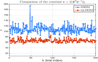
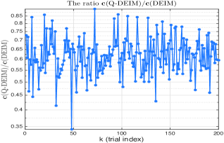
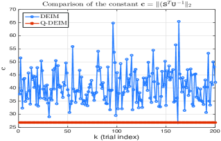
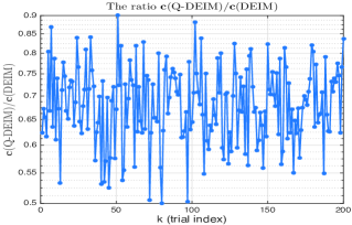
We illustrate the difference in the values of computed by DEIM and Q-DEIM using randomly generated orthonormal matrices of size . The Q-DEIM selection not only enjoys better upper bound, but it also in most cases provides smaller actual value of , as seen on Figure 1. It is interesting to note that all Q-DEIM values of are below , sustaining the conjectured bound for the volume maximizing scheme. On the other hand, DEIM breaches the upper bound in most of the trials, indicating less optimal selection with respect to the volume maximizing criterion. In the case of matrices specially constructed to exhibit large pivot growth, the value of in both methods may exceed , but not with a big factor. We also compare DEIM and Q-DEIM using a basis for a FitzHugh-Naguma system, analyzed in detail in §2.2.1. The value of for Q-DEIM is fixed at , independent of the orthogonal changes of the basis.
2.1.1 Implementation details
In terms of the row selection from , the actual computation used in Theorem 2 is an LQ factorization of with row pivoting. The transposition and QR with column pivoting is used only for convenience and due to the availability of software implementations. A Householder based QR factorization of a fat matrix runs with complexity , similar to the complexity of DEIM. LAPACK [1] based software tools use the optimized, BLAS 3 based and robust [20] function xGEQP3. Other pivoting strategies are possible, such as in xGEQPX, xGEQPY in [10], [11]. On parallel computing machinery, our new approach uses the best available QR code with column pivoting; e.g. PxGEQPF from ScaLAPACK [12].
As an illustration of the simplicity at which we get high performance computation of a good selection operator, and to make a case for Q-DEIM, we briefly describe a MATLAB implementation. Using the notation of Theorem 2, we have
| (22) |
The computation by a triangular solver (e.g. the backslash \ or linsolve() in MATLAB) is numerically stable as is well conditioned and . The explicitly set identity matrix in (22) guarantees that the selected entries of a vector will be exactly interpolated when is computed as in (22). If is computed as (e.g. by MATLAB’s slash) then , with all at roundoff level. If are the interpolation indices selected by , then checking the interpolation for yields
revealing an undesirable pollution of , in particular if .
2.1.2 DEIM and LU with partial pivoting
It has been known, at least to experts, that DEIM is a variation of Gaussian elimination; Sorensen [40, 38] called it a pivoted LU without replacement. Recently, [2] proposed to replace Step 7 of Algorithm 1, , by (To make the distinction clear, we denote the new variable by and we use to denote the matrix at the end of the th step.). In other words, the basis is updated by adding the current residual vector. Assume that at step , , where is unit upper triangular and that both computations have the same selection (this holds at ). Then the residual is easily shown to be the same as in Algorithm 1. Hence, the updated will be the same, and , with an updated unit upper triangular .
Note that is lower triangular at each step: The upper triangular part of the last column of this product is , which is zero by the definition of . Therefore, with a lower trapezoidal and a unit upper triangular . Hence, DEIM (with replacement) is the same as a row pivoted LU decomposition. This connection might help understanding why DEIM behaves much better than the theoretical upper bound would suggest. Similar to the discussion in Remark 4, DEIM is applying a locally greedy search to maximize the volume of : Because with a unit upper triangular , , and the ’s are results of a greedy search for maxima.
The modified update yielding reduces the computational complexity of to down from + because the LU decomposition of is no longer necessary. However, the claim in [2] that Algorithm 1 contains complexity is misleading because a practical implementation of Step 5, , will not compute the LU decomposition of from scratch in each step. Instead, it will exploit the fact that, in the step, is changed by appending only a new row and a column and will update the LU decomposition with complexity ; thus making the total complexity of Algorithm 1 of + .
This connection also suggests using a rank revealing LU decomposition of with complete pivoting and taking the indices of the first pivoted rows as the DEIM indices. The bound on changes only by a factor originating from the inverse of the unit upper triangular LU factor, which, as a consequence of complete pivoting, is bounded by . On the other hand, in the case of partial pivoting like in DEIM, the bound is rather pessimistic. However, as expected, DEIM behaves much better in practice, as partial LU hardly exhibits the worst case growth scenario. It is an interesting challenge to determine what orthonormal basis of the range of is best for the performances of DEIM.
2.2 Model Reduction Examples
In this section, we test the performance of the new selection procedure on two model reduction benchmark problems.
2.2.1 The FitzHugh-Naguma (F–N) System
The F–N system, a simplified version of the Hodgkin–Huxley model, arises in modeling the activation and deactivation dynamics of a spiking neuron. This example is borrowed from [39] and we follow their description of the model, including their notation and parameter selection. Let and denote, respectively, the voltage and recovery of voltage. Also, let and . Then, the underlying dynamics are described by the coupled nonlinear PDEs
| (23) | |||||
| (24) |
with the nonlinearity appearing as and with the initial and boundary conditions
where the model parameters are chosen as , , , , and the stimulus . A finite difference discretization leads to a system of the form (1) with system dimension . A time-domain simulation with equally spaced points for leads to state and nonlinear snapshots. Following [39], we choose and perform model reduction using both DEIM selection procedures. We simulate both reduced models, collect reduced-order snapshots and . Then, to measure the error in model reduction, we lift these two snapshots back to the original dimension, i.e., we compute and where is the POD basis for model reduction, and measure their distance (in the relative Frobenius-norm) from the original snapshot . Let and denote the resulting errors. For , we obtain and .
To illustrate that this is the usual behavior, i.e., the Q-DEIM selection performs as well as the original DEIM selection, we test other values as well:
To better illustrate the comparison, we measure, in relative -norm, how accurately each entry of is reconstructed with DEIM and Q-DEIM. Therefore, we measure the relative -norm distance between the rows of the original snapshot matrix and those of the reconstructed ones and . The results are shown in Figure 2, once more, illustrating that both procedures perform equally well.

2.2.2 Nonlinear RC Model
This is a model of nonlinear RC-ladder circuit [16, 4, 7]222The model can be downloaded from Max Planck Institute Model Reduction Wiki page at http://morwiki.mpi-magdeburg.mpg.de/morwiki/index.php/Nonlinear-RC-Ladder., another benchmark example for model reduction. The nonlinearity results from resistors that are in a parallel connection with diodes; the diode I-V characteristics have the nonlinearity where is the current through the diode and is the voltage across it. The input is the current source entering at node .
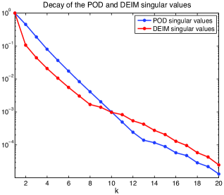
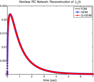
We take , i.e., connect such ladders and excite the system using the exponential forcing . A numerical simulation over seconds results in POD snapshots and nonlinear (DEIM) snapshots . Decay of the POD and DEIM singular values are shown in the left-hand side plot of Figure 3. Based on this decay, we pick and apply POD with both DEIM and Q-DEIM selections. In this example, the voltage at node , i.e., the first component of (denoted by ), is the quantity of interest and we measure how both reduced models approximate . As shown on Figure 3, both methods perform extremely well; the reduced-model quantities are virtually indistinguishable from the original.
As in the previous example, we compute the reconstruction errors due to DEIM and Q-DEIM, and obtain and ; once again high accuracy for both models. The reconstruction errors in due to DEIM and Q-DEIM are and respectively. Once we increase to , both reduced models become even more accurate with and . The reconstruction errors in are now for DEIM and for Q-DEIM.
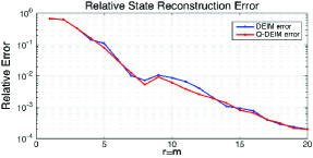
To further illustrate the dependence of the error on the reduced dimension, we test both DEIM and Q-DEIM for . The results depicted in Figure 4 below confirm the earlier observations.
The two other excitation selections suggested for this model are and [17]. For these two inputs, for all the and combinations we have tried, DEIM and Q-DEIM have returned exactly the same selection matrix ; resulting in exactly same reduced model that is very accurate, with relative errors of even with . For brevity, we omit the resulting figures.
3 Using restricted/randomized basis information
The framework introduced in §2 allows various modifications. Here we describe one, introducing Q-DEIMr, a version of Q-DEIM that works only on a random selection of the rows of . This introduces the techniques of randomized sampling in the theory and practice of DEIM, but it also provides a new approach to sampling from orthonormal matrices [30].
If the dimension is large, it would be advantageous to determine a good selection operator in a way to reduce the factor in the complexity of the algorithm. From the proof of Theorem 2 it follows that, for the quality of the DEIM projection, we only need to ensure that the upper triangular matrix has small inverse. But is the pivoted QR triangular factor of certain columns of , and our initial task is to find their indices; we have no interest in the QR factorization as such. This immediately suggests that we may attempt to find such indices using only a small selection of the columns of (i.e. of the rows of ).333In another situation, e.g. in a case of gappy POD approximation, we may want to avoid some rows of because e.g. they correspond to spatial coordinates with corrupted or missing information.
The following scheme depicts the main idea: suppose we randomly sample columns of (marked by ) and assemble them in a local working array .
| (25) |
Then we attempt QR with column pivoting on with a built-in Incremental Condition Estimator (ICE) that at any step very efficiently estimates the norm of the inverse of the thus far constructed part of the triangular factor .444Here we assume that the triangular factor overwrites the corresponding part of the array .
This is done as follows: Suppose the first steps have been successful and the computed triangular factor ( in (26)) is well conditioned. The corresponding global column indices (in ) that correspond to these columns in are stored and removed from the active set of indices from which random selection is made. All Householder reflectors used are accumulated in a matrix .
In the th step, a new pivot column is selected and swapped to be the th one, and the single Householder reflector is applied only to that column to annihilate its positions to , and to compute the th position, ( in (26)). At this moment we have all the ingredients to compute the value (marked as in (26)). If is below given threshold, the factorization continues by accepting the pivotal column, completing the th step and looking for the next pivot. If not, it means that the th position, ( in (26)) is too small, and, due to pivoting, that all entries in the active submatrix of ( in (26)) are also small. In that case, the columns to in are useless for our purposes and we discard them and draw new columns from the active set of columns of ( in (25)). Before using newly selected columns as a part of , we need to update them by applying unitary matrix which contains accumulated all previous transformations. The resulting new columns in ( in (26)) can now participate in pivoting.
| (26) |
At this point we may simply choose to continue with the factorization, search for the next pivot column, swap it to the th position, test against the threshold and accept if it passes the test, as illustrated in (26). Another option is to discard all previous pivoting and start a completely new one by determining the largest column for the first position, and proceed with a completely new pivoting process on the updated contents of . The value of is not necessarily fixed and may change dynamically with a safety device to prevent failure. With proper data structure, one can develop a detailed algorithm and an efficient software implementation. For the sake of brevity, we omit the details. However, we provide one illustrative example.
Example 6.
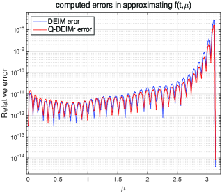
Let , , . Take uniformly sampled values of and compute the snapshots over the discretized –domain at uniformly spaced nodes. The best low rank approximation of the sampled returned with columns. This indicates that the POD basis has captured the function’s behavior. We allowed Q-DEIMr to process only columns in the work array , and set the upper bound for at555This ad hoc choice is motivated by the structure of the upper bound for , as in the proof of Theorem 2. Note that we use instead of the worst case theoretical bound. . Column index drawing is done simply: “random” indices are taken as the leading indices of randomly permuted active set. We stress here that the purpose of this example is to illustrate the idea and its potential, to motivate further study of the randomized sampling approach to DEIM projection.
After processing rows of (out of ), Q-DEIMr selected a submatrix with ; DEIM processed the whole matrix and returned . To test how well the two methods approximate , we compute its value at points in the –interval: for each the function is evaluated over the –grid giving . The same is done with DEIM and Q-DEIM projections giving and , respectively. The results of a comparison are depicted in Figure 5.
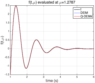
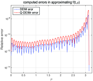

Since at this point no sophisticated sampling strategy is used, the results may vary, depending on , , and the given upper bound for . Figure 6 illustrates how the prescribed upper bound for changes the execution and performance of Q-DEIMr. By visiting only rows, we fully recover the accuracy achieved by using all rows of .
Remark 7.
The technical details of using ICE in the above procedure are similar to the rank revealing method with windowed column pivoting [11]. However, the overall procedure is substantially different in spirit. The difference is that our objective is not to compute a rank revealing QR factorization (we know that is of full row rank, , and we do not even need its QR factorization), but just to find a well conditioned submatrix. This allows to touch only a selection of columns of and exit when a sufficiently well conditioned submatrix is determined.
Remark 8.
The quest for a well-conditioned submatrix of can be obviously parallelized, and many processors can independently work on different (not necessarily disjoint) subsets of column indices, with no need whatsoever to engage in communication, until one finds suitable columns and sends a halt signal. If more than one selection is found, the best one will be chosen.
The column selection procedure can be improved at a cost of one pass through the array to compute the column norms . Such additional information can be used e.g. in the following two ways:
Select from the sorted columns in batches, as needed, starting from the largest ones. The norms of the columns in the active set can also be down-dated, using the procedure from column pivoted QR with numerically robust implementation [20].
Define , . Then is a probability distribution that can be used to draw column samples. It prefers larger columns. Each column is used only once, and the distribution is computed for the active set.
This opens a completely new aspect of DEIM and establishes its connection to randomized numerical linear algebra, in particular with randomized sampling of rows of orthonormal matrices [30]. In particular, one can view Q-DEIMr as a guided randomized sampling algorithm for orthonormal matrices. Detailed analysis of blending the two procedures is omitted here; it will be available in our subsequent work.
Remark 9.
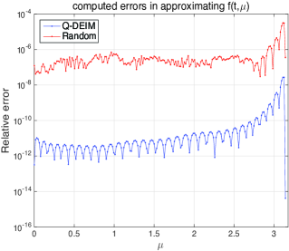
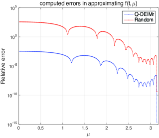
Our experiments with randomized selection indicate that merely picking random interpolation indices will not work in general and sophisticated strategies of DEIM, Q-DEIM, Q-DEIMr are necessary for a reliable and robust black-box procedure. Indeed, this is already revealed in Example 6; the initial random selection is not enough and Q-DEIMr brings in additional rows to process. Clearly, the results depend on the function being approximated but just to illustrate the importance of the selection principle of DEIM and Q-DEIMr, below we show the reconstruction accuracy of DEIM and randomly selected indices (with few trials to select better rows, but without the condition number control as in Q-DEIMr) for two nonlinear parametrized functions. As the figures illustrate, the random selection without the techniques from the DEIM procedures may perform very poorly.
4 Conclusions and Future Work
Using the tools from QR factorization with column pivoting, this paper has introduced a new DEIM index selection strategy, that is invariant under orthogonal transformations, with a sharper error bound for the DEIM projection error. The new approach, called Q-DEIM, is tested on several numerical examples and it performs as well as the original DEIM selection procedure. For the cases of large dimensions, a modification is proposed that uses only randomly sampled rows of the data matrix yet still leading to high-fidelity approximations.
In addition to the nonlinear model reduction and parametrized function settings we presented here, the new Q-DEIM selection is well suited for several important applications that we are currently investigating for our subsequent work. One such application is randomized sampling of rows of orthonormal matrices for solving the least-squares problems effectively in the cases with huge row dimension. The second one is the DEIM induced CUR factorization recently introduced by Sorensen and Embree [41]. A third application arises in nonlinear inversion and parametric model reduction, see, e.g., [8, 18], where an affine decomposition is needed for a parametric matrix for efficient online model reduction step. This is usually handled by vectorizing which might lead to very large row dimension depending on the sparsity pattern of . We are currently testing Q-DEIM and Q-DEIMr in these settings. Further, both DEIM and Q-DEIM (including Q-DEIMr) can adopt an updating scheme when the nonlinear snapshot basis is obtained by the SVD: one can enlarge and incrementally to yield better approximations. In Q-DEIM, increasing will require updating a rank-revealing QR-decomposition; thus finding an efficient updating scheme for this incremental implementation will prove very useful.
5 Acknowledgments
We would like to thank Dr. Saifon Chaturantabut for providing the data and code for the FitzHugh-Naguma Model Example in §2.2.1, and Dr. Christopher Beattie, Dr. Mark Embree and Dr. Danny Sorensen for various enlightening discussions. The work of Drmač was supported by the grant HRZZ-9345 from the Croatian Science Foundation, in part by the NSF through grant DMS-1217156, and by the Interdisciplinary Center for Applied Mathematics during his research visit to the Department of Mathematics at Virginia Tech in the 2014-2015 Academic Year. The work of Gugercin was supported in part by the NSF through grant DMS-1217156. The authors acknowledge partial support of the Einstein Foundation and of the Technische Universität Berlin during the completion of this work, and we thank Dr. Christopher Beattie and Dr. Volker Mehrmann for hosting us in Berlin.
References
- [1] E. Anderson, Z. Bai, C. Bischof, L. S. Blackford, J. Demmel, J. J. Dongarra, J. Du Croz, S. Hammarling, A. Greenbaum, A. McKenney, and D. Sorensen, LAPACK Users’ Guide (Third Ed.), Society for Industrial and Applied Mathematics, Philadelphia, PA, USA, 1999.
- [2] H. Antil, S. E. Field, F. Herrmann, R. H. Nochetto, and M. Tiglio, Two-step greedy algorithm for reduced order quadratures, Journal of Scientific Computing, 57 (2013), pp. 604–637.
- [3] P. Astrid, S. Weiland, K. Willcox, and T. Backx, Missing point estimation in models described by proper orthogonal decomposition, IEEE Transactions on Automatic Control, (2008), pp. 2237–2251.
- [4] Z. Bai and D. Skoogh, A projection method for model reduction of bilinear dynamical systems, Linear Algebra and its Applications, 415 (2006), pp. 406–425.
- [5] M. Barrault, N. C. Nguyen, Y. Maday, and A. T. Patera, An empirical interpolation method: Application to efficient reduced-basis discretization of partial differential equations, C. R. Acad. Sci. Paris, Série I., 339 (2004), pp. 667–672.
- [6] P. Benner and T. Breiten, Interpolation-based -model reduction of bilinear control systems, SIAM Journal on Matrix Analysis and Applications, 33 (2012), pp. 859–885.
- [7] P. Benner and T. Breiten, Two-sided projection methods for nonlinear model order reduction, SIAM Journal on Scientific Computing, 37 (2015), pp. B239–B260.
- [8] P. Benner, S. Gugercin, and K. Willcox, A survey of model reduction methods for parametric systems, Tech. Rep. MPIMD/13-14, Max Planck Institute Magdeburg Preprint, August 2013.
- [9] G. Berkooz, P. Holmes, and J. Lumley, The proper orthogonal decomposition in the analysis of turbulent flows, Annual Review of Fluid Mechanics, 25 (1993), pp. 539–575.
- [10] C. H. Bischof and G. Quintana-Orti, Algorithm 782: codes for rank–revealing QR factorizations of dense matrices, ACM Transactions on Mathematical Software, 24 (1998), pp. 254–257.
- [11] , Computing rank–revealing QR factorizations of dense matrices, ACM Transactions on Mathematical Software, 24 (1998), pp. 226–253.
- [12] L. S. Blackford, J. Choi, A. Cleary, E. D’Azeuedo, J. Demmel, I. Dhillon, S. Hammarling, G. Henry, A. Petitet, K. Stanley, D. Walker, and R. C. Whaley, ScaLAPACK User’s Guide, Society for Industrial and Applied Mathematics, Philadelphia, PA, USA, 1997.
- [13] P. A. Businger and G. H. Golub, Linear least squares solutions by Householder transformations, Numerische Mathematik, 7 (1965), pp. 269–276.
- [14] K. Carlberg, C. Farhat, J. Cortial, and D. Amsallem, The GNAT method for nonlinear model reduction: Effective implementation and application to computational fluid dynamics and turbulent flows, Journal of Computational Physics, 242 (2013), pp. 623–647.
- [15] S. Chandrasekaran and I. C. F. Ipsen, On rank–revealing factorizations, SIAM Journal on Matrix Analysis and Applications, 15 (1994), pp. 592–622.
- [16] Y. Chen, Model order reduction for nonlinear systems, Master’s thesis, Massachusetts Institute of Technology, 1999.
- [17] M. Condon and R. Ivanov, Model reduction of nonlinear systems, COMPEL-The international journal for computation and mathematics in electrical and electronic engineering, 23 (2004), pp. 547–557.
- [18] E. de Sturler, S. Gugercin, M. Kilmer, S. Chaturantabut, C. Beattie, and M. O’Connell, Nonlinear parametric inversion using interpolatory model reduction, SIAM Journal on Scientific Computing, to appear; arXiv:1311.0922, (2015).
- [19] Z. Drmač, A global convergence proof for cyclic Jacobi methods with block rotations, SIAM Journal on Matrix Analysis and Applications, 31 (2009), pp. 1329–1350.
- [20] Z. Drmač and Z. Bujanović, On the failure of rank revealing QR factorization software – a case study, ACM Trans. Math. Softw., 35 (2008), pp. 1–28.
- [21] R. Everson and L. Sirovich, The Karhunen-Loeve Procedure for Gappy Data, Journal of the Optical Society of America, 12 (1995), pp. 1657–1664.
- [22] D. Faddeev, V. Kublanovskaya, and V. Faddeeva, Solution of linear algebraic systems with rectangular matrices., Proc. Steklov Inst. Math., 96 (1968), pp. 93–111.
- [23] G. Flagg and S. Gugercin, Multipoint Volterra series interpolation and optimal model reduction of bilinear systems, To appear in SIAM Journal on Matrix and Analysis and Applications, (2015). Available as arXiv preprint arXiv:1312.2627.
- [24] K. Glover, All optimal Hankel-norm approximations of linear multivariable systems and their -error bounds, International journal of control, 39 (1984), pp. 1115–1193.
- [25] S. Goreinov, E. Tyrtyshnikov, and N. Zamarashkin, A theory of pseudoskeleton approximations, Linear Algebra and its Applications, 261 (1997), pp. 1 – 21.
- [26] C. Gu, QLMOR: a projection-based nonlinear model order reduction approach using quadratic-linear representation of nonlinear systems, Computer-Aided Design of Integrated Circuits and Systems, IEEE Transactions on, 30 (2011), pp. 1307–1320.
- [27] S. Gugercin, A. Antoulas, and C. Beattie, model reduction for large-scale linear dynamical systems, SIAM Journal on Matrix Analysis and Applications, 30 (2008), pp. 609–638.
- [28] M. Hinze and S. Volkwein, Proper orthogonal decomposition surrogate models for nonlinear dynamical systems: Error estimates and suboptimal control, in Dimension Reduction of Large-Scale Systems, Springer, 2005, pp. 261–306.
- [29] H. Hotelling, Analysis of a complex of statistical variables with principal components, Journal of Educational Psychology, 24 (1933), pp. 417–441,498–520.
- [30] I. C. F. Ipsen and T. Wentworth, The effect of coherence on sampling from matrices with orthonormal columns, and preconditioned least squares problems, SIAM Journal on Matrix Analysis and Applications, 35 (2014), pp. 1490–1520.
- [31] W. Kahan, Numerical linear algebra, Canadian Mathematical Bulletin, 9 (1965), pp. 757–801.
- [32] K. Kunisch and S. Volkwein, Galerkin proper orthogonal decomposition methods for a general equation in fluid dynamics, SIAM Journal on Numerical analysis, 40 (2002), pp. 492–515.
- [33] C. L. Lawson and R. J. Hanson, Solving Least Squares Problems, Prentice–Hall Inc., Englewood Cliffs, N. J., 1974.
- [34] M. Loéve, Probability Theory, D. Van Nostrand Company Inc., New York, 1955.
- [35] J. Lumley, The Structures of Inhomogeneous Turbulent Flow, Atmospheric Turbulence and Radio Wave Propagation, (1967), pp. 166–178.
- [36] B. Moore, Principal component analysis in linear systems: Controllability, observability, and model reduction, IEEE Transactions on Automatic Control, 26 (1981), pp. 17–32.
- [37] C. Mullis and R. Roberts, Synthesis of minimum roundoff noise fixed point digital filters, IEEE Transactions on Circuits and Systems, 23 (1976), pp. 551–562.
- [38] S. S. Chaturantabut and D. Sorensen., Nonlinear model reduction for porous media flow, in 2010 SIAM Annual Meeting, 2010.
- [39] S. S. Chaturantabut and D. Sorensen, Nonlinear model reduction via discrete empirical interpolation, SIAM Journal on Scientific Computing, 32 (2010), pp. 2737–2764.
- [40] D. Sorensen. Private communications, 2010.
- [41] D. C. Sorensen and M. Embree, A DEIM induced CUR factorization, CAAM Department Technical Report TR14-04, Rice University, July 2014.