Compton scattering of twisted light: angular distribution and polarization of scattered photons

Abstract

Compton scattering of twisted photons is investigated within a non-relativistic framework using first-order perturbation theory. We formulate the problem in the density matrix theory, which enables one to gain new insights into scattering processes of twisted particles by exploiting the symmetries of the system. In particular, we analyze how the angular distribution and polarization of the scattered photons are affected by the parameters of the initial beam such as the opening angle and the projection of orbital angular momentum. We present analytical and numerical results for the angular distribution and the polarization of Compton scattered photons for initially twisted light and compare them with the standard case of plane-wave light.

I Introduction

The inelastic scattering of photons on (quasi-)free charged particles, known also as the Compton scattering of light, is one of the best studied processes in quantum mechanics. This process demonstrates that light is more than a classical wave phenomenon and that quantum theory is required in order to explain the frequency shifts as well as the angular and polarization distribution of the scattered light Compton (1923); Klein and Nishina (1929). For example, the classical electro-magnetic theory cannot properly describe the frequency shifts at low intensity of the incident photons Jackson (1983), although these shifts are derived quite easily from the conservation of the (total) energy and momentum of the quantum particles involved in the scattering. In the framework of quantum theory, a shift in the wavelength of the photons occurs since, for an electron at rest, for example, a part of the incident photon energy is transferred to the recoil of the electron. Therefore, an elastic scattering of the light can only be assumed if the photon energy is negligible, compared to the rest energy of the electrons. This low-energy limit to the Compton scattering of photons can be described by the non-relativistic Schrödinger theory Greiner (1989).

Indeed, derivations of the angular distribution and polarization of the Compton scattered light can be found in many texts but are made usually for plane-wave photons and electrons Greiner (1989); Berestetzki et al. (1980). Such a plane-wave approximation to the Compton scattering applies if the lateral sizes of the incident electron and photon beams are (much) larger than their wavelength. In contrast, less attention has been paid to the Compton scattering of “twisted” beams in which each photon (or electron) carries an non-zero projection of the orbital angular momentum (OAM) along the propagation direction, in addition to the spin angular momentum that is related to the polarization of the light Allen et al. (1992); O’Neil et al. (2002); Molina-Terriza et al. (2007); Yao and Padgett (2011); Andrews and Babiker (2013). Here, we therefore investigate how an OAM of the incident radiation affects the angular distribution and polarization of the (Compton) scattered light. In particular, we apply the density matrix formalism Blum (2012) to explore the angular distribution and polarization of the scattered light and compare this to the results of a plane-wave scattering. Calculations of the angle-differential Compton cross sections have been performed for the scattering of Bessel beams with different opening angles and total angular momenta $m$. While the cross section does not depend on $m$, it is highly sensitive with regard to the opening angle $\theta_{k}$ of the Bessel beams. Moreover, the formulation of the problem within the density matrix theory clearly highlights why the results do not depend on $m$. This can be explained as restriction to those elements of the twisted state photonic density matrix that are diagonal in the momentum quantum numbers due to the spatial symmetries of the system.

This work is structured as follows. In Sec. II, we briefly review the non-relativistic description of Compton scattering in the framework of the density matrix theory. This includes a short account on the electron-photon interaction in the non-relativistic framework as well as the quantization of the photon field. We derive the density matrix of the Compton scattered photons in terms of the usual plane-wave matrix elements which are weighted by the initial photonic density matrix in a plane-wave basis. The standard case of plane-wave Compton scattering is presented for later reference in Sec. III. The description of twisted photon states is presented in Sec. IV. Detailed calculations have been performed for the angular distribution and polarization of Compton scattered twisted photons, and will be explained in comparison with the plane-wave case. A short summary is finally given in Sec. V. In the Appendix, in addition, we collect all issues related to the normalization of the plane-wave and twisted-wave one-particle states and their density matrices.

II Density Matrix Theory for non-relativistic Compton scattering

We consider the scattering of plane-wave or twisted photons on either a beam of free electrons as emitted from an electron gun Englert and Rinehart (1983), or on a target material with a low work function, much lower than the frequency of light, such that the electrons can be considered as quasi-free. Twisted light has been produced in a wide range of frequencies Cojoc et al. (2006); Yao and Padgett (2011); Zürch et al. (2012); Hemsing et al. (2013); Bahrdt et al. (2013); Gariepy et al. (2014). If the frequency of the photon $\omega$ in the rest frame of the electron is much smaller than the electron rest energy, i.e. if the recoil parameter

$$r=\frac{\hbar\omega}{m_{\mathrm{e}}c^{2}}\ll 1\,,$$ (1)

we can work in the low-energy limit of non-relativistic Compton scattering. We then conveniently work in the rest frame of the incident electron, where the theoretical description of the scattering process is much easier. For an electron beam target the results observed in the laboratory frame where the electrons are moving can be obtained by just performing a proper Lorentz transformation. For electron beams with low kinetic energy, $E_{\rm kin}\lesssim$1\text{\,}\mathrm{keV}$$, the quantitative results in the rest frame and the laboratory frame differ very little. The size of the target should be larger than the lateral size of the vortex light beam Arlt and Dholakia (2000); Kumar et al. (2010); Andrews and Babiker (2013). Throughout the paper we use units with $\hbar=1$ unless stated otherwise. Moreover, we employ Gaussian units, where the fine-structure constant $\alpha=e^{2}$.

II.1 Density Matrix Formalism

To describe the angular distribution and polarization of the scattered photons it is most convenient to use the density-matrix theory Blum (2012); Balashov et al. (2000). The density matrix formalism has been applied just recently to describe the interaction of twisted light with many-electron atoms and ions Surzhykov et al. (2015). In this formalism, the system after the collision is described by the final state density operator $\hat{\rho}_{f}$, which is related to the density operator of the system in the initial state before the scattering, $\hat{\rho}_{i}$, by the scattering operator,

$$\hat{\rho}_{f}=\hat{S}\hat{\rho}_{i}\hat{S}^{\dagger}\,,$$ (2)

and where $\hat{S}$ characterizes the interaction of the particles during the collision.

Before the scattering, the electrons and photons are initially independent and uncorrelated. The density operator of the initial state can thus be written as the direct product of the electronic ($\hat{\rho}_{i}^{\mathrm{el}}$) and photonic ($\hat{\rho}_{i}^{\mathrm{ph}}$) operators Surzhykov et al. (2015)

$$\hat{\rho}_{i}=\hat{\rho}_{i}^{\mathrm{el}}\otimes\hat{\rho}_{i}^{\mathrm{ph}}\,.$$ (3)

We describe the initial electron as a plane-wave in a pure quantum state $|\boldsymbol{p}_{i}\rangle$ with the density operator $\hat{\rho}_{i}^{\mathrm{el}}=|\boldsymbol{p}_{i}\rangle\langle\boldsymbol{p}_{i}|$. The initial photon is described by the initial state photonic density operator $\hat{\rho}_{\gamma}\equiv\hat{\rho}_{i}^{\mathrm{ph}}(\gamma)$, where $\gamma$ refers to a set of quantum numbers to describe that state. Below, we will specify the quantum numbers $\gamma$ that are needed to represent either a plane-wave or a twisted-wave photon.

Let us now write the final state density operator $\hat{\rho}_{f}$ in a matrix representation in a plane-wave basis, where $|f\rangle=|\boldsymbol{p}_{f},\boldsymbol{k}_{f}\Lambda_{f}\rangle$ abbreviates the final plane-wave electron and photon states, where $\boldsymbol{p}_{f}$ denotes the final electron momentum while $\boldsymbol{k}_{f}$ and $\Lambda_{f}$ stand for the final photon momentum and helicity, respectively. Let us also introduce complete sets of initial plane-wave states $|i\rangle=|\boldsymbol{p},\boldsymbol{k}\lambda\rangle$, with $\sumint\limits_{i}|i\rangle\langle i|=1$ (for a detailed discussion of the orthonormality and completeness of these plane-wave bases see the Appendix), to obtain the density matrix in the following form:

$$\langle f\hskip 1.00006pt|\hskip 1.00006pt\hat{\rho_{f}}\hskip 1.00006pt|\hskip 1.00006ptf^{\prime}\rangle=\\ \sumint\limits_{\lambda,\lambda^{\prime}}\widetilde{\mathrm{d}\boldsymbol{k}}\widetilde{\mathrm{d}\boldsymbol{k}}^{\prime}\,\langle\boldsymbol{k}\lambda\hskip 1.00006pt|\hskip 1.00006pt\hat{\rho}_{\gamma}\hskip 1.00006pt|\hskip 1.00006pt\boldsymbol{k}^{\prime}\lambda^{\prime}\rangle\langle\boldsymbol{p}_{i},\boldsymbol{k}^{\prime}\Lambda^{\prime}\hskip 1.00006pt|\hskip 1.00006pt\hat{S}^{\dagger}\hskip 1.00006pt|\hskip 1.00006ptf^{\prime}\rangle\langle f\hskip 1.00006pt|\hskip 1.00006pt\hat{S}\hskip 1.00006pt|\hskip 1.00006pt\boldsymbol{p}_{i},\boldsymbol{k}\Lambda\rangle\,,$$ (4)

where we employed the fact that the initial electron is in a plane wave state as discussed above, and where $\widetilde{\mathrm{d}\boldsymbol{k}}$ is an abbreviation for the properly normalized integration measure (for details we refer to the Appendix). This equation states that in order to calculate the final state density matrix for an arbitrary initial photon state $\hat{\rho}_{\gamma}$, either plane-wave or a twisted-wave or any other photon state, we just need to know the ordinary plane-wave $S$ matrix elements to describe the physics. Equation (4) describes how these plane-wave $S$ matrix elements have to be weighted by the elements of the initial photonic density matrix in the plane-wave basis $\langle\boldsymbol{k}\lambda\hskip 1.00006pt|\hskip 1.00006pt\hat{\rho}_{\gamma}\hskip 1.00006pt|\hskip 1.00006pt\boldsymbol{k}^{\prime}\lambda^{\prime}\rangle$.

The elements of the $S$ matrix themselves can be represented in a form

$$\langle f\hskip 1.00006pt|\hskip 1.00006pt\hat{S}\hskip 1.00006pt|\hskip 1.00006pti\rangle=-2\pi i\delta(E_{i}-E_{f})\langle f\hskip 1.00006pt|\hskip 1.00006pt\hat{T}\hskip 1.00006pt|\hskip 1.00006pti\rangle\,,$$ (5)

where the delta function ensures the conservation of energy, i.e. the total energy of the initial state particles $E_{i}$ equals the total energy of the final state particles $E_{f}$. The matrix elements of the transition operator $\hat{T}$ can be calculated using perturbation theory Greiner (1989).

The normalization of the density matrix is purely conventional and for us it is most convenient to normalize it to the total cross section. This is achieved by dividing out the flux of incident particles Taylor (1972):

$$\sigma:=\frac{{\rm tr}\,\hat{\rho}_{f}}{TV{\rm tr}\,(\hat{J}\hat{\rho}_{i})}\,,$$ (6)

where $T$ and $V$ are the interaction time and volume, respectively. In order to calculate the cross section for twisted particles, which are spatially localized, we need a convenient definition of flux density operator $\hat{J}$ in terms of the densities of colliding particles times their relative velocity Landau and Lifschitz (1992). Since twisted beams are not spatially homogeneous perpendicular to their propagation direction, a proper definition of the cross section according to the book of Taylor Taylor (1972) includes an average over the lateral structure of the beam of incident particles. We conclude that we should define the cross section by means of the spatially averaged density of the initial particles $\langle n\rangle:=V^{-1}\int\!\mathrm{d}^{3}x\,n(\boldsymbol{x})$ that is proportional to the trace of the initial state density operator $\langle n\rangle={\rm tr}\,\hat{\rho}/V$. Thus, the operator of the averaged density is just the unity operator divided by the quantization volume $V$ (see the Appendix), and the flux density operator $\hat{J}$ in (6) can be represented as $\hat{J}=c\frac{\hat{1}_{\mathrm{el}}}{V}\otimes\frac{\hat{1}_{\mathrm{ph}}}{V}$, i.e. by the relative velocity, the speed of light $c$, times the operators of the averaged particle densities of electrons and photons in the initial state.

Using the basis expansion of the density operator, Eq. (4), and by employing the energy conservation in (5) we find that the cross section (6) contains a factor $\delta(E_{f}-E_{i})\delta(E_{f}-E_{i^{\prime}})=\delta(E_{f}-E_{i})\delta(E_{i}-E_{i^{\prime}})$. For a non-zero contribution to the scattering cross section, the total energies of the initial state bases used for the expansion of the final state density matrix, Eq. (4), need to be equal. Finally, we can express the scattering cross section as

$$\sigma=\frac{2\pi V}{c\,{\rm tr}\,\hat{\rho}_{\gamma}}\sumint\limits_{f}\sumint\limits_{\lambda,\lambda^{\prime}}\widetilde{\mathrm{d}\boldsymbol{k}}\widetilde{\mathrm{d}\boldsymbol{k}}^{\prime}\delta(E_{i}-E_{f})\\ \times\langle\boldsymbol{k}\lambda\hskip 1.00006pt|\hskip 1.00006pt\hat{\rho}_{\gamma}\hskip 1.00006pt|\hskip 1.00006pt\boldsymbol{k}^{\prime}\lambda^{\prime}\rangle\langle\boldsymbol{p}_{i},\boldsymbol{k}^{\prime}\lambda^{\prime}\hskip 1.00006pt|\hskip 1.00006pt\hat{T}^{\dagger}\hskip 1.00006pt|\hskip 1.00006ptf\rangle\langle f\hskip 1.00006pt|\hskip 1.00006pt\hat{T}\hskip 1.00006pt|\hskip 1.00006pt\boldsymbol{p}_{i},\boldsymbol{k}\lambda\rangle\,.$$ (7)

Here we already employed the normalization of the initial electron plane-wave states ${\rm tr}\,\hat{\rho}_{i}^{\mathrm{el}}=\langle\boldsymbol{p}_{i}\hskip 1.00006pt|\hskip 1.00006pt\boldsymbol{p}_{i}\rangle=1$. This concludes our general discussion of the density matrix formalism and the definition of the cross section. The main result of this section is the representation of the final-state density matrix (4) of Compton scattered light for an incident plane-wave or twisted-wave photon beam—characterized by the photonic density operator $\hat{\rho}_{\gamma}$—in terms of the plane-wave matrix elements for the interaction of electrons and photons.

II.2 Interaction Between Photons and Electrons

Let us now turn our attention on the description of the interaction between the electrons and the photons. The form of the interaction Hamiltonian,

$$\hat{H}_{\mathrm{int}}=\frac{e\hat{\boldsymbol{A}}\cdot\hat{\boldsymbol{p}}}{m_{\mathrm{e}}c}+\frac{e^{2}\hat{\boldsymbol{A}}^{2}}{2m_{\mathrm{e}}c^{2}}\,,$$ (8)

follows from the gauge invariant minimal coupling of the electromagnetic field to the free electron Hamiltonian Greiner (1989). The operator $\hat{\boldsymbol{A}}$ of the electromagnetic vector potential describes the emission or the absorption of one photon Greiner (1989). Compton scattering is a two-photon process: The incident photon is absorbed by the electron while the scattered photon is emitted into some other direction. The one-photon interaction operator $\hat{\boldsymbol{A}}\cdot\hat{\boldsymbol{p}}$ does not contribute to the non-relativistic Compton scattering amplitude, because the matrix elements of the electron momentum operator $\hat{p}$ vanish in the rest frame of the electron Greiner (1989). Thus, the Compton scattering amplitude can be calculated in first-order perturbation theory by means of the two-photon contribution $\hat{\boldsymbol{A}}^{2}$ to the Hamiltonian; the transition matrix elements are just given by $\langle f\hskip 1.00006pt|\hskip 1.00006pt\hat{T}\hskip 1.00006pt|\hskip 1.00006pti\rangle=\langle f\hskip 1.00006pt|\hskip 1.00006pt\hat{H}_{\mathrm{int}}\hskip 1.00006pt|\hskip 1.00006pti\rangle$.

The photon field operator $\hat{\boldsymbol{A}}$ that enters the interaction Hamiltonian, Eq. (8), can be represented by its mode expansion into a circularly polarized plane-wave basis $\boldsymbol{u}_{\boldsymbol{k}\Lambda}(\boldsymbol{x})=e^{i\boldsymbol{k}\cdot\boldsymbol{x}}\,\boldsymbol{\varepsilon}_{\boldsymbol{k}\Lambda}$, where the polarization vector $\boldsymbol{\varepsilon}_{\boldsymbol{k}\Lambda}$ is perpendicular to the wave-vector, $\boldsymbol{k}\cdot\boldsymbol{\varepsilon}_{\boldsymbol{k}\Lambda}=0$. There are two independent solutions for each $\boldsymbol{k}$, denoted by the photon helicity $\Lambda=\pm 1$. In terms of these plane-wave modes the photon field operator is given by

$$\hat{\boldsymbol{A}}(\boldsymbol{x})=\sumint\limits_{\Lambda}\!\widetilde{\mathrm{d}\boldsymbol{k}}\,N_{k}\left[\hat{c}_{\boldsymbol{k}\Lambda}\boldsymbol{u}_{\boldsymbol{k}\Lambda}(\boldsymbol{x})+\hat{c}_{\boldsymbol{k}\Lambda}^{\dagger}\boldsymbol{u}_{\boldsymbol{k}\Lambda}^{*}(\boldsymbol{x})\right]\,,$$ (9)

where we employ the proper integration measure $\widetilde{\mathrm{d}\boldsymbol{k}}$ to “count” the basis functions (see the Appendix for details). The creation operator $\hat{c}^{\dagger}_{\boldsymbol{k}\Lambda}$ creates a normalized one-photon plane-wave state from the vacuum $|\boldsymbol{k}\Lambda\rangle=\hat{c}^{\dagger}_{\boldsymbol{k}\Lambda}|0\rangle$ that is characterized by its linear momentum (wave-vector) $\boldsymbol{k}$ and helicity $\Lambda$. The one-photon states are normalized as $\langle\boldsymbol{k}\Lambda\hskip 1.00006pt|\hskip 1.00006pt\boldsymbol{k}\Lambda\rangle=1$. Moreover, the normalization factor $N_{k}=\sqrt{2\pi c/kV}$ is determined such that the energy eigenvalues of the free field Hamiltonian are just $\omega_{k}=c|\boldsymbol{k}|$ for one-photon states $|\boldsymbol{k}\Lambda\rangle$ Greiner (1989). It is sufficient to know the above representation of the photon field operator in a plane-wave basis because we just need to calculate the plane-wave matrix elements by means of Eqs. (4) and (7).

II.3 The Reduced Density Matrix of Compton Scattered Photons

We are going to investigate the angular distribution and polarization of the scattered photons, and we are not interested in the electron distribution after the scattering has occurred. We therefore have to calculate a reduced density matrix $\rho_{\Lambda^{\prime}\Lambda}(\boldsymbol{k}_{f}/k_{f})$, which depends on the direction of the scattered photon $\boldsymbol{k}_{f}/k_{f}$ and its polarization state $\Lambda$, by tracing out the unobserved final electron states. We obtain the reduced density matrix of the Compton scattered photons

$$\rho_{\Lambda^{\prime}\Lambda}(\boldsymbol{k}_{f}/k_{f})=\frac{V^{2}}{(2\pi)^{2}c\,{\rm tr}\,{\hat{\rho}_{\gamma}}}\sumint\limits_{\lambda,\lambda^{\prime}}\!\widetilde{\mathrm{d}\boldsymbol{k}}\widetilde{\mathrm{d}\boldsymbol{k}}^{\prime}\,\int\!\widetilde{\mathrm{d}\boldsymbol{p}_{f}}\,\int\!\mathrm{d}k_{f}k_{f}^{2}\,\delta(E_{f}-E_{i})\,\langle\boldsymbol{k}\lambda\hskip 1.00006pt|\hskip 1.00006pt\hat{\rho}_{\gamma}\hskip 1.00006pt|\hskip 1.00006pt\boldsymbol{k}^{\prime}\lambda^{\prime}\rangle\,\mathcal{M}^{*}_{\boldsymbol{k}^{\prime}\lambda^{\prime}}(\Lambda^{\prime})\mathcal{M}_{\boldsymbol{k}\lambda}(\Lambda)\,,$$ (10)

in terms of the plane-wave matrix elements $\mathcal{M}_{\boldsymbol{k}\lambda}(\Lambda)=\langle\boldsymbol{p}_{f};\boldsymbol{k}_{f}\Lambda\hskip 1.00006pt|\hskip 1.00006pt\hat{H}_{\mathrm{int}}\hskip 1.00006pt|\hskip 1.00006pt\boldsymbol{p}_{i};\boldsymbol{k}\lambda\rangle$. The calculation of the plane-wave matrix elements for non-relativistic Compton scattering can be found in textbooks, e.g. in Greiner (1989), and we only cite here the final result:

$$\mathcal{M}_{\boldsymbol{k}\lambda}(\Lambda) =\frac{e^{2}}{m_{\mathrm{e}}c^{2}}\frac{2\pi c^{2}}{L^{3}}\,\frac{\boldsymbol{\varepsilon}_{\boldsymbol{k}_{f}\Lambda}^{*}\cdot\boldsymbol{\varepsilon}_{\boldsymbol{k}\lambda}}{\sqrt{\omega_{i}\omega_{f}}}\,\widetilde{\delta}(\boldsymbol{p}_{i}+\boldsymbol{k}-\boldsymbol{k}_{f}-\boldsymbol{p}_{f})\,.$$ (11)

Here, $\tilde{\delta}$ denotes a normalized delta function with the property $\tilde{\delta}(0)=1$. For details we refer to the Appendix. Because the reduced density matrix (10) contains the product of two plane-wave matrix elements we also get two delta functions that ensure the conservation of momentum. Their product can be reformulated as,

$$\widetilde{\delta}(\boldsymbol{p}_{i}+\boldsymbol{k}-\boldsymbol{p}_{f}-\boldsymbol{k}_{f})\widetilde{\delta}(\boldsymbol{p}_{i}+\boldsymbol{k}^{\prime}-\boldsymbol{p}_{f}-\boldsymbol{k}_{f})\\ =\widetilde{\delta}(\boldsymbol{k}^{\prime}-\boldsymbol{k})\widetilde{\delta}(\boldsymbol{p}_{f}+\boldsymbol{k}_{f}-\boldsymbol{p}_{i}-\boldsymbol{k})\,,$$ (12)

where we obtain a factor $\widetilde{\delta}(\boldsymbol{k}^{\prime}-\boldsymbol{k})$, which consumes one of the integrations over the plane-wave bases, $\widetilde{\mathrm{d}\boldsymbol{k}^{\prime}}$, in Eq. (10). For this reason, only those elements of the initial state photonic density matrix with $\boldsymbol{k}=\boldsymbol{k}^{\prime}$ remain in Eq. (10). Thus, just the momentum-diagonal elements of $\hat{\rho}_{\gamma}$ contribute to the reduced density matrix of the scattered photons and the coherences in the off-diagonal elements of the initial photonic density matrix are lost. The reason for this behaviour is of course the momentum conservation in the plane-wave matrix elements that is related to the spatial homogeneity of the system via Noether’s theorem Noether (1918). All particles are described as plane-waves, except for the initial photons that are prepared in the hitherto unspecified quantum state $\hat{\rho}_{\gamma}$. It is the spatial homogeneity of the residual system of incident and scattered particles which excludes the interference of different momentum components of the initial photonic state $\hat{\rho}_{\gamma}$ from the reduced density matrix (10) of the scattered photons.

The above momentum conservation, together with the conservation of the total energy $\delta(E_{f}-E_{i})=\delta(\omega_{f}+p_{f}^{2}/2m_{\mathrm{e}}-\omega-p_{i}^{2}/2m_{\mathrm{e}})$, determines the frequency of the scattered photons. Recalling that we work in the rest frame of the incident electron, $\boldsymbol{p}_{i}=0$, we find for the frequency of the scattered photons

$$\omega_{f}=\omega\left[1-\frac{\hbar\omega}{m_{\mathrm{e}}c^{2}}(1-\cos\theta){+O\left(\frac{\hbar\omega}{m_{\mathrm{e}}c^{2}}\right)^{2}}\right]\,,$$ (13)

where we temporarily reinstated $\hbar$. The expression for $\omega_{f}$ in (13) accounts for the well-known frequency red-shift of Compton scattering Compton (1923), which depends on the angle $\theta$ between the initial and the scattered photon momentum vectors. When starting from a fully relativistic QED calculation, we would get the above non-relativistic frequency shift in (13) the leading order of an expansion in the small recoil parameter $r$, Eq. (1). Because of Eq. (13), the length of the scattered photon’s wave-vector $|\boldsymbol{k}_{f}|=\omega_{f}(\theta)/c$ is completely determined by its direction.

In the electric dipole approximation, the momentum of the photon and its recoiling effect on the electron is neglected, $\boldsymbol{k}=\boldsymbol{k}_{f}=0$. This is a good approximation whenever the recoil parameter, Eq. (1), is negligibly small. The non-relativistic Compton scattering becomes elastic within the dipole approximation: $\omega_{f}=\omega$. Moreover, the dipole approximation coincides with the formal classical limit $\hbar\to 0$. Within the dipole approximation we obtain as final formula for the elements of the reduced density matrix the following expression:

$$\rho_{\Lambda^{\prime}\Lambda}(\boldsymbol{k}_{f}/k_{f})=\frac{e^{4}}{m_{\mathrm{e}}^{2}c^{4}}\sumint\limits_{\lambda,\lambda^{\prime}}\!\widetilde{\mathrm{d}\boldsymbol{k}}\,\,\frac{\langle\boldsymbol{k}\lambda\hskip 1.00006pt|\hskip 1.00006pt\hat{\rho}_{\gamma}\hskip 1.00006pt|\hskip 1.00006pt\boldsymbol{k}\lambda^{\prime}\rangle}{{\rm tr}\,{\hat{\rho}_{\gamma}}}\,\left(\boldsymbol{\varepsilon}_{\boldsymbol{k}_{f}\Lambda^{\prime}}^{*}\cdot\boldsymbol{\varepsilon}_{\boldsymbol{k}\lambda^{\prime}}\right)^{*}\left(\boldsymbol{\varepsilon}_{\boldsymbol{k}_{f}\Lambda}^{*}\cdot\boldsymbol{\varepsilon}_{\boldsymbol{k}\lambda}\right)\,.$$ (14)

II.4 Stokes parameters and differential cross section

In the previous subsection we calculated a suitable expression for the reduced density matrix of Compton scattered photons, Eq. (14). We now relate the elements of the reduced density matrix to the angular distribution of the scattered photons, i.e. to their angular differential cross section and the polarization properties. According to Blum (2012); Balashov et al. (2000), the reduced density matrix can be represented by the three Stokes parameters $\boldsymbol{P}=(P_{1},P_{2},P_{3})$ via

$$\rho_{\Lambda^{\prime}\Lambda}(\boldsymbol{k}_{f})=\frac{\mathrm{d}\sigma}{\mathrm{d}\Omega}\,\frac{1}{2}\begin{pmatrix}1+P_{3}&P_{1}-iP_{2}\\ P_{1}+iP_{2}&1-P_{3}\end{pmatrix}_{\Lambda^{\prime}\Lambda}\,.$$ (15)

From this representation it is easy to obtain the angular differential cross section of Compton scattered photons as

$$\frac{\mathrm{d}\sigma}{\mathrm{d}\Omega}=\sum_{\Lambda=\pm 1}\rho_{\Lambda\Lambda}(\boldsymbol{k}_{f})=\rho_{+1+1}+\rho_{-1-1}\,.$$ (16)

The Stokes parameters are given by

$$P_{1} =\frac{\rho_{+1-1}+\rho_{-1+1}}{\rho_{+1+1}+\rho_{-1-1}}\,,$$ (17)

$$P_{2} =\frac{i\rho_{+1-1}-i\rho_{-1+1}}{\rho_{+1+1}+\rho_{-1-1}}\,,$$ (18)

$$P_{3} =\frac{\rho_{+1+1}-\rho_{-1-1}}{\rho_{+1+1}+\rho_{-1-1}}\,.$$ (19)

As usual, the Stokes parameters $P_{1}$ and $P_{2}$ represent the intensity of light that is linearly polarized under different angles with respect to the scattering plane. The scattering plane is defined by the direction of the incident beam of light and by the momentum vector of the scattered photon. The Stokes parameter $P_{3}$ measures the amount of light with circular polarization Balashov et al. (2000); McMaster (1961). Moreover, the degree of polarization $\mathrm{\Pi}$ is defined as the length of the vector $\boldsymbol{P}$

$$\mathrm{\Pi}=\sqrt{P_{1}^{2}+P_{2}^{2}+P_{3}^{2}}\,.$$ (20)

This concludes our discussion of the density matrix formalism. We are now ready to study the angular distribution and the polarization properties of Compton scattered light for both plane-wave and twisted photons.

III Compton Scattering of Plane-wave Photons

Let us now apply the formalism to the standard case of the Compton scattering of plane-wave photons, as a starting point for later comparison with the case of twisted light. Moreover, this will convince us that we normalized the reduced density matrix correctly to obtain the differential cross section by comparing with the well known results from the literature.

We now specify the initial photon state as a plane wave with wave-vector $\boldsymbol{k}_{i}$ and in a well defined helicity state $\Lambda_{i}$, with the photonic initial density operator $\hat{\rho}_{\gamma}=\hat{\rho}_{\boldsymbol{k}_{i}\Lambda_{i}}=|\boldsymbol{k}_{i}\Lambda_{i}\rangle\langle\boldsymbol{k}_{i}\Lambda_{i}|$. It has the following representation in a plane-wave basis:

$$\langle\boldsymbol{k}\lambda\hskip 1.00006pt|\hskip 1.00006pt\hat{\rho}_{\boldsymbol{k}_{i}\Lambda_{i}}\hskip 1.00006pt|\hskip 1.00006pt\boldsymbol{k}^{\prime}\lambda^{\prime}\rangle=\widetilde{\delta}(\boldsymbol{k}-\boldsymbol{k}^{\prime})\delta_{\lambda\lambda^{\prime}}\widetilde{\delta}(\boldsymbol{k}-\boldsymbol{k}_{i})\delta_{\lambda\Lambda_{i}}\,.$$ (21)

Using its diagonal elements $\langle\boldsymbol{k}\lambda\hskip 1.00006pt|\hskip 1.00006pt\hat{\rho}_{\boldsymbol{k}_{i}\Lambda_{i}}\hskip 1.00006pt|\hskip 1.00006pt\boldsymbol{k}\lambda^{\prime}\rangle=\delta_{\lambda\lambda^{\prime}}\delta_{\lambda\Lambda_{i}}\widetilde{\delta}(\boldsymbol{k}-\boldsymbol{k}_{i})$ into Eq. (14) readily yields the reduced density matrix of non-relativistic Compton scattering of circularly polarized plane-wave photons in the dipole approximation

$$\rho_{\Lambda^{\prime}\Lambda}(\boldsymbol{k}_{f}) =r_{\mathrm{e}}^{2}\left(\boldsymbol{\varepsilon}_{\boldsymbol{k}_{f}\Lambda^{\prime}}^{*}\cdot\boldsymbol{\varepsilon}_{\boldsymbol{k}_{i}\Lambda_{i}}\right)^{*}\left(\boldsymbol{\varepsilon}_{\boldsymbol{k}_{f}\Lambda}^{*}\cdot\boldsymbol{\varepsilon}_{\boldsymbol{k}_{i}\Lambda_{i}}\right)\,,$$ (22)

where $r_{\mathrm{e}}=e^{2}/(m_{\mathrm{e}}c^{2})\simeq$2.8\text{\,}\mathrm{fm}$$ is the classical electron radius.

To become more specific, we need to specify the scattering geometry, and to express the photon polarization vectors in terms of the scattering angles. Let us assume that the initial photon beam propagates along the $z$-axis, $\boldsymbol{k}_{i}/k_{i}=(0,0,1)^{T}$, while the scattered photon propagates into the direction $\boldsymbol{k}_{f}/k_{f}=(\sin\theta\cos\varphi,\,\sin\theta\sin\varphi,\,\cos\theta)^{T}$, where the scattering angle $\theta$ and azimuthal angle $\varphi$ are the usual polar and azimuthal angles in spherical coordinates. For the polarization vectors of the scattered photons we give the explicit representation

$$\boldsymbol{\varepsilon}_{\boldsymbol{k}_{f}\Lambda}=\boldsymbol{\varepsilon}_{\Lambda}(\theta,\varphi)=\frac{1}{\sqrt{2}}\begin{pmatrix}\cos\theta\cos\varphi-i\Lambda\sin\varphi\\ \cos\theta\sin\varphi+i\Lambda\cos\varphi\\ -\sin\theta\end{pmatrix}\,,$$ (23)

which makes evident that the polarization vector is orthonormalized $\boldsymbol{\varepsilon}_{\boldsymbol{k}_{f}\Lambda}^{*}\cdot\boldsymbol{\varepsilon}_{\boldsymbol{k}_{f}\Lambda^{\prime}}=\delta_{\Lambda\Lambda^{\prime}}$ and perpendicular to the momentum direction $\boldsymbol{k}_{f}\cdot\boldsymbol{\varepsilon}_{\boldsymbol{k}_{f}\Lambda}=0$. Because the incident photon propagates along the $z$-axis, its polarization vector is just $\boldsymbol{\varepsilon}_{\boldsymbol{k}_{i}\Lambda_{i}}=\boldsymbol{\varepsilon}_{\Lambda_{i}}(0,0)=(1/\sqrt{2},i\Lambda_{i}/\sqrt{2},0)^{T}$.

The differential Compton cross section as a function of the scattering angle is just given by using the representations (23) of the photons polarization vectors into Eq. (22), and by summing over the final state polarization according to Eq. (16). This yields

$$\frac{\mathrm{d}\sigma_{\mathrm{pw}}}{\mathrm{d}\Omega}=\frac{r_{\mathrm{e}}^{2}}{2}(1+\cos^{2}\theta)\,,$$ (24)

where $\theta$ denotes the scattering angle, i.e. the angle between the wave-vectors of the incident and the scattered light. The result (24) for the angular differential cross section of Compton scattered light in the dipole approximation is well known and can also be obtained by means of classical electrodynamics Jackson (1983). An integration of Eq. (24) over all directions of the scattered photons just yields the well known total Thomson cross section $\sigma=\frac{8}{3}\pi r_{\mathrm{e}}^{2}\simeq$665\text{\,}\mathrm{mb}$$. This comparison with well-known results from the literature shows that we normalized the final state density matrix correctly to the cross section.

Similarly to the cross section, we can obtain explicit expressions for the three Stokes parameters of the scattered photons as

$$P_{1} =-\frac{\sin^{2}\theta}{1+\cos^{2}\theta}\,,$$ (25)

$$P_{2} =0\,,$$ (26)

$$P_{3} =\frac{2\Lambda_{i}\cos\theta}{1+\cos^{2}\theta}\,.$$ (27)

As we see from Eqs. (25) – (27), the scattered photons are not necessarily circularly polarized, although the initial photons were. The ratio of the amount of linearly and circularly polarized photons varies with the scattering angle $\theta$. For instance, under $\theta=$90\text{\,}\mathrm{\SIUnitSymbolDegree}$$ we have $P_{1}=-1$ and the photons are completely linearly polarized in the direction perpendicular to the scattering plane. Nevertheless, the scattered photons are fully polarized, $\mathrm{\Pi}=1$, independent of the scattering angle. This concludes our short review of the analytic results for the differential cross section and the Stokes parameters for plane-wave photons. We will pick them up in the next section where we compare them with the case Compton scattering of twisted light.

IV Compton Scattering of Twisted-wave Photons

We now turn to the main aspect of our paper: The calculation of the angular distribution and the polarization properties of Compton scattered twisted light. For that, we need first to construct the initial photonic density matrix for twisted photons.

IV.1 Description of Twisted Photon States and the Twisted Photon Density Matrix

The state of a photon in a Bessel beam that propagates along the $z$-axis, briefly referred to as a Bessel-state or twisted photon, is characterized by its longitudinal momentum $\kappa_{\parallel}$, i.e. the component of the linear momentum along the beam’s propagation axis, the modulus of the transverse momentum $\kappa_{\perp}=|\boldsymbol{k}_{\perp}|$, the projection of the total angular momentum (TAM) onto the propagation axis $m$, and the photon helicity $\Lambda$ Matula et al. (2013). A photon in a twisted one-particle Bessel-state is, thus, characterized by the quantum numbers $|\gamma\rangle=|\kappa_{\perp}\kappa_{\parallel}m\Lambda\rangle$. It can be represented by a coherent superposition of plane-wave states Jentschura and Serbo (2011a); Ivanov (2011); Matula et al. (2013); Surzhykov et al. (2015),

$$|\kappa_{\perp}\kappa_{\parallel}m\Lambda\rangle=\int\!\widetilde{\mathrm{d}\boldsymbol{k}}\,b_{\kappa_{\perp}\kappa_{\parallel}m}(\boldsymbol{k})\,|\boldsymbol{k}\Lambda\rangle\,,$$ (28)

where we use the proper integration measure $\widetilde{\mathrm{d}\boldsymbol{k}}$ for plane-wave states (see the Appendix). From Eq. (28) we see that $\Lambda$ refers to the helicity of the plane-wave components of the twisted photon. The amplitudes $b_{\kappa_{\perp}\kappa_{\parallel}m}(\boldsymbol{k})$ are given by

$$b_{\kappa_{\perp}\kappa_{\parallel}m}(\boldsymbol{k})=N_{\rm tw}\,\delta(k_{z}-\kappa_{\parallel})\,a_{\kappa_{\perp}m}(\boldsymbol{k}_{\perp})$$ (29)

and are related to the usually employed transverse amplitudes (see e.g. Jentschura and Serbo (2011a); Matula et al. (2013); Surzhykov et al. (2015))

$$a_{\kappa_{\perp}m}(\boldsymbol{k}_{\perp})=\sqrt{\frac{2\pi}{\kappa_{\perp}}}(-i)^{m}e^{im\varphi_{k}}\delta(|\boldsymbol{k}_{\perp}|-\kappa_{\perp})\,.$$ (30)

Because for a photon in a twisted Bessel state $\kappa_{\parallel}$ and $\kappa_{\perp}$ are well-defined, all the momentum vectors $\boldsymbol{k}$ of the superposition (28) are lying on a cone in momentum space with fixed opening angle $\theta_{k}=\arctan(\kappa_{\perp}/\kappa_{\parallel})$. The direction of the momentum vector $\boldsymbol{k}$ on the cone is undefined, and can be parametrized as

$$\boldsymbol{k}=\boldsymbol{k}(\varphi_{k})=\begin{pmatrix}\kappa_{\perp}\cos\varphi_{k}\\ \kappa_{\perp}\sin\varphi_{k}\\ \kappa_{\parallel}\end{pmatrix}=k\begin{pmatrix}\sin\theta_{k}\cos\varphi_{k}\\ \sin\theta_{k}\sin\varphi_{k}\\ \cos\theta_{k}\end{pmatrix}\,.$$ (31)

where $\varphi_{k}$ is the azimuthal angle that defines the orientation of one particular vector $\boldsymbol{k}(\varphi_{k})$ on the momentum cone. The length of these vectors, $k=|\boldsymbol{k}(\varphi_{k})|=\sqrt{\kappa_{\parallel}^{2}+\kappa_{\perp}^{2}}$, are related to the photon frequency $\omega=ck$ as for plane-waves.

The normalization factor $N_{\rm tw}=\sqrt{4\pi^{3}/L_{z}RV}$ that appears in the definition of the amplitudes $b_{\kappa_{\perp}\kappa_{\parallel}m\Lambda}$ is determined such that the twisted one-particle states are orthonormalized in the following way:

$$\langle\kappa_{\perp}\kappa_{\parallel}m\Lambda\hskip 1.00006pt|\hskip 1.00006pt\kappa_{\perp}^{\prime}\kappa_{\parallel}^{\prime}m^{\prime}\Lambda^{\prime}\rangle\\ =\frac{2\pi^{2}}{RL_{z}}\delta_{mm^{\prime}}\delta_{\Lambda\Lambda^{\prime}}\delta(\kappa_{\perp}-\kappa_{\perp}^{\prime})\delta(\kappa_{\parallel}-\kappa_{\parallel}^{\prime})$$ (32)

and $\langle\kappa_{\perp}\kappa_{\parallel}m\Lambda\hskip 1.00006pt|\hskip 1.00006pt\kappa_{\perp}\kappa_{\parallel}m\Lambda\rangle=1$. This corresponds to the normalization to one particle per cylindrical volume $V=\pi R^{2}L_{z}$, where both the radius $R$ and the length $L_{z}$ of the cylinder are going to infinity (see the Appendix).

Let us now construct the density operator for twisted photons in the pure quantum state (28), together with its matrix representation in a plane-wave basis. The latter is needed to calculate the reduced density matrix, Eq. (14), of Compton scattered twisted light. The normalization of the one-photon states implies that the twisted-state density operator

$$\hat{\rho}_{\gamma}=\hat{\rho}_{\kappa_{\perp}\kappa_{\parallel}m\Lambda}=|\kappa_{\perp}\kappa_{\parallel}m\Lambda\rangle\langle\kappa_{\perp}\kappa_{\parallel}m\Lambda|$$ (33)

has unity trace, ${\rm tr}\,(\hat{\rho}_{\kappa_{\perp}\kappa_{\parallel}m\Lambda})=1$, i.e. it is normalized to an average particle density of “one particle per volume $V$”. The matrix elements of the twisted density operator (33) in a plane-wave basis are just given by products of the amplitudes $b_{\kappa_{\perp}\kappa_{\parallel}m\Lambda}$, Eq. (29),

$$\langle\boldsymbol{k}\lambda\hskip 1.00006pt|\hskip 1.00006pt\hat{\rho}_{\kappa_{\perp}\kappa_{\parallel}m\Lambda}\hskip 1.00006pt|\hskip 1.00006pt\boldsymbol{k}^{\prime}\lambda^{\prime}\rangle =\delta_{\lambda\lambda^{\prime}}\delta_{\lambda\Lambda}\,b_{\kappa_{\perp}\kappa_{\parallel}m}(\boldsymbol{k})\,b^{*}_{\kappa_{\perp}\kappa_{\parallel}m}(\boldsymbol{k}^{\prime})$$

$$\propto\delta_{\lambda\lambda^{\prime}}\delta_{\lambda\Lambda}e^{im(\varphi_{k}-\varphi_{k}^{\prime})}$$ (34)

and they are diagonal in the helicity quantum numbers. We stress that only the momentum-off-diagonal elements of the density matrix (34) do depend on the projection of total angular momentum $m$. It enters as the difference of the vortex phase factors $e^{im\varphi_{k}}$ of the two plane-wave components $\boldsymbol{k}\neq\boldsymbol{k}^{\prime}$. On the other hand, the momentum-diagonal elements of the above density matrix

$$\langle\boldsymbol{k}\lambda\hskip 1.00006pt|\hskip 1.00006pt\hat{\rho}_{\kappa_{\perp}\kappa_{\parallel}m\Lambda}\hskip 1.00006pt|\hskip 1.00006pt\boldsymbol{k}\lambda^{\prime}\rangle\\ =\delta_{\lambda\lambda^{\prime}}\delta_{\lambda\Lambda}\frac{(2\pi)^{2}}{V\kappa_{\perp}}\delta(k_{z}-\kappa_{\parallel})\delta(|\boldsymbol{k}_{\perp}|-\kappa_{\perp})\,$$ (35)

which enter the calculation of the reduced density matrix of Compton scattered photons, Eq. (14), are completely independent of $m$. Therefore, also the angular distribution and polarization of the Compton scattered photons do not dependent of $m$.

A few remarks might be in order why the reduced density matrix of the scattered photons is independent from $m$. In this paper we are interested in the angular distribution and polarization properties of the Compton scattered photons. We, therefore, project the final state density operator onto a basis of plane-wave states that can be observed by a usual detector, which measures the linear momentum of a photon Ivanov (2011). Thus, all involved particles except for the initial twisted photons are described as plane-wave states. From the discussion in the previous section we know that the momentum conservation described by the delta function in the plane-wave matrix elements enforces the restriction to the momentum-diagonal elements of the initial photonic density matrix. Thus, we loose the dependence on $m$ because only the momentum-diagonal elements of the photonic density matrix (34) that describes the initial twisted state contribute due to symmetries of the system.

It is known from previous studies that the scattering of twisted particles on spatially homogeneous systems, such as plane-waves Ivanov (2011); Seipt et al. (2014), impact-parameter averaged atomic targets Scholz-Marggraf et al. (2014); Surzhykov et al. (2015), impact-parameter averaged potential scattering , leads to angular distributions of the scattered particles or fluorescence light that are independent of $m$. On the other hand, the coherences of the initial state density matrix will play a role for scenarios with a spatial inhomogeneity other than the twisted beam. For instance the angular distributions do depend on $m$ for the collision of a twisted particle with an inhomogeneous target, like: a second beam of twisted particles Ivanov (2011, 2012), a localized microscopic target such as a single atom Lloyd et al. (2012); Matula et al. (2013); Van Boxem et al. (2014); Van Boxem et al. (2015); Surzhykov et al. (2015), or a quantum dot Quinteiro et al. (2015).

Another possibility to recover the coherences in the off-diagonal elements of the twisted density matrix is to look for the angular momentum of the scattered particles. In fact, it has been shown in Jentschura and Serbo (2011a, b) that Compton backscattered photons do indeed carry orbital angular momentum. In order to access the angular momentum of the scattered photons, one needs to determine the final-state density operator $\hat{\rho}_{f}$ in the the basis of the twisted states. This requires a suitable detection operator that directly measures the orbital angular momentum of the scattered photons Balashov et al. (2000); Ivanov (2011); Jentschura and Serbo (2011a).

IV.2 Angular distribution and Stokes parameters for the scattering of a twisted photon with well-defined TAM

If we substitute the initial state density matrix (35) of the twisted photon into Eq. (14), and by performing the integration over the plane-wave basis in cylindrical coordinates $\int\!\widetilde{\mathrm{d}\boldsymbol{k}}=\frac{V}{(2\pi)^{3}}\int\!\mathrm{d}\varphi_{k}\mathrm{d}k_{z}\mathrm{d}k_{\perp}k_{\perp}$, we obtain the reduced density matrix for the Compton scattering of a twisted photon (in the dipole approximation $\omega_{f}=\omega_{i}$) . It includes an integration over all plane-wave components as described by $\varphi_{k}$

$$\rho_{\Lambda^{\prime}\Lambda}=r_{\mathrm{e}}^{2}\int\!\frac{\mathrm{d}\varphi_{k}}{2\pi}\left(\boldsymbol{\varepsilon}_{\boldsymbol{k}_{f}\Lambda^{\prime}}^{*}\cdot\boldsymbol{\varepsilon}_{\boldsymbol{k}(\varphi_{k})\Lambda_{i}}\right)^{*}\left(\boldsymbol{\varepsilon}_{\boldsymbol{k}_{f}\Lambda}^{*}\cdot\boldsymbol{\varepsilon}_{\boldsymbol{k}(\varphi_{k})\Lambda_{i}}\right)\,,$$ (36)

with $\boldsymbol{k}(\varphi_{k})$ from Eq. (31). This reduced density matrix can be directly compared with the corresponding result for plane-wave light, Eq. (22).

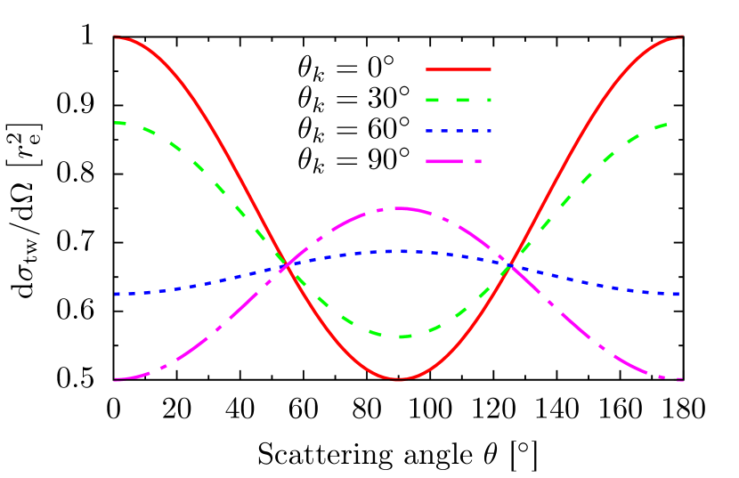
Figure 1: (Color online) Differential cross section $\mathrm{d}\sigma_{\mathrm{tw}}/\mathrm{d}\Omega$ for Compton scattering of twisted light as a function of the scattering angle $\theta$. Results are shown for various values of the momentum cone opening angle $\theta_{k}$ of the twisted photons. The case $\theta_{k}=0$ is equivalent to plane-wave photons. Of course, the limit $\theta_{k}\to$90\text{\,}\mathrm{\SIUnitSymbolDegree}$$ of large cone opening angles can not be reached experimentally.

If we make use of the explicit representation of the polarization vectors (23), the integration over the azimuthal angle $\varphi_{k}$ in Eq. (36) can be carried out and yields the differential cross section

$$\frac{\mathrm{d}\sigma_{\mathrm{tw}}}{\mathrm{d}\Omega}=\frac{r_{\mathrm{e}}^{2}}{4}\left[(1+\cos^{2}\theta_{k})(1+\cos^{2}\theta)+2\sin^{2}\theta_{k}\sin^{2}\theta\right]\,,$$ (37)

where $\theta$ denotes the scattering angle measured from the $z$-axis, and $\theta_{k}=\arctan\kappa_{\perp}/\kappa_{\parallel}$ denotes the opening angle of the initial twisted photon beam. As anticipated above, the differential cross section is independent of the value of the projection of total angular momentum $m$, but it does depend on the momentum cone opening angle $\theta_{k}$. Note that in the limit $\theta_{k}\to 0$ we recover the plane-wave result (24).

The results for the differential cross section is shown in Fig. 1 as function of the scattering angle $\theta$ for various cone angles $\theta_{k}$. The red solid curve ($\theta_{k}=0$) corresponds to the case of initial plane-wave photons and shows the well known symmetric angular distribution which is minimal at the scattering angle $\theta=$90\text{\,}\mathrm{\SIUnitSymbolDegree}$$, where it is just $1/2$ of the value at forward or backward scattering. For increasing values of the cone opening angle $\theta_{k}>0$ the angular distribution of the scattered photons gradually changes and the dip at $\theta=$90\text{\,}\mathrm{\SIUnitSymbolDegree}$$ becomes less pronounced. For sufficiently large $\theta_{k}>\theta_{k}^{\star}$ the distribution turns around with the maximum of the angular distribution occurring at $\theta=$90\text{\,}\mathrm{\SIUnitSymbolDegree}$$ (e.g. for the blue dotted curve in Fig. 1). This crossover occurs at the “magic angle” of $\theta_{k}^{\star}=\arccos(1/\sqrt{3})\approx$54.7\text{\,}\mathrm{\SIUnitSymbolDegree}$$, where the angular distribution is flat.

(a) Stokes Parameter $P_{1}$	(b) Stokes Parameter $P_{3}$	(c) Degree of polarization $\Pi$

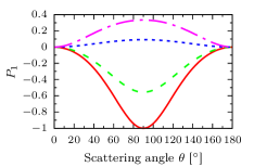
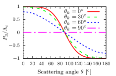
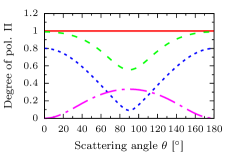
Figure 2: (Color online) The polarization of Compton scattered photons is characterized by the Stokes parameters $P_{1}$ (left), $P_{3}$ (middle) and the degree of polarization $\mathrm{\Pi}$ (right) as a function of the scattering angle. Results are shown for beams of twisted photons with different momentum cone opening angles $\theta_{k}$. As in Fig. 1, the case $\theta_{k}=0$ is equivalent to plane-wave photons.

In addition to the angular distribution discussed above, the momentum cone opening angle $\theta_{k}$ of the twisted photon beam also influences the polarization properties of the Compton scattered light. For incident photons in the Bessel state, the Stokes parameters are given by

$$P_{1} =\frac{(1-3\cos^{2}\theta_{k})\sin^{2}\theta}{(1+\cos^{2}\theta_{k})(1+\cos^{2}\theta)+2\sin^{2}\theta_{k}\sin^{2}\theta}\,,$$ (38)

$$P_{2} =0\,,$$ (39)

$$P_{3} =\frac{4\Lambda_{i}\cos\theta_{k}\cos\theta}{(1+\cos^{2}\theta_{k})(1+\cos^{2}\theta)+2\sin^{2}\theta_{k}\sin^{2}\theta}\,.$$ (40)

Similar to the differential cross section, the Stokes parameters do neither depend on the azimuthal angle of the scattered photon, nor on the total angular momentum $m$ of the incident twisted beam, as the whole scenario is cylindrically symmetric. Again the results for the plane-wave case are reproduced for $\theta_{k}=0$.

The results for the Stokes parameters are shown in Fig. 2 as function of the scattering angle $\theta$ for different opening angles $\theta_{k}$. As discussed above for plane-wave photons, the values of $P_{1}$ and $P_{3}$, which quantify the linear and circular polarization of the scattered radiation, respectively, depend on the scattering angle. Both values are sensitive to the cone opening angle $\theta_{k}$ of the twisted light. For instance, as depicted in Fig. 2 (a), the value of $P_{1}$ at $90\text{\,}\mathrm{\SIUnitSymbolDegree}$ scattering decreases in magnitude for increasing values of $\theta_{k}$, starting from $P_{1}=-1$ for the plane-wave case ($\theta_{k}=0$). In particular, for the “magic angle” of $\theta_{k}^{\star}=\arccos(1/\sqrt{3})$ the scattered photons are not linearly polarized, since $P_{1}=0$ for all scattering angles. For even larger $\theta_{k}>\theta_{k}^{\star}$ the value of $P_{1}$ is positive which indicates a change of the plane of linear polarization of the scattered photons which are now (partially) polarized in the scattering plane. Since the sign of $P_{3}$ depends on the helicity $\Lambda_{i}=\pm 1$ of the incident photons, we show in Fig. 2 (b) the combination $P_{3}/\Lambda_{i}$ instead. The values of $P_{3}$ gradually decrease for increasing $\theta_{k}$, and approach zero for $\theta_{k}\to$90\text{\,}\mathrm{\SIUnitSymbolDegree}$$. For twisted light with $\theta_{k}>0$, the degree of polarization is smaller than $1$, so the scattered photons are not fully polarized anymore. For not too large cone opening angles $\theta_{k}$ the scattered radiation is depolarized the strongest at $\theta=$90\text{\,}\mathrm{\SIUnitSymbolDegree}$$. For sufficiently large $\theta_{k}$ angular dependence of the degree of polarization shows the opposite behavior. In particular for $\theta_{k}\to$90\text{\,}\mathrm{\SIUnitSymbolDegree}$$ the scattered radiation becomes completely depolarized for forward and backward scattering, while the degree of polarization $\mathrm{\Pi}$ is nonzero at finite scattering angles, see Fig. 2 (c).

IV.3 Angular distribution for the scattering of a superposition of twisted photons

As discussed above, the angular distribution of Compton scattered photons and their polarization does not depend on the value of the total angular momentum $m$ if the initial light is prepared in a Bessel state with well-defined $m$; it just depends on the opening angle $\theta_{k}$ of the beam.

We now examine the Compton scattering of a coherent superposition of two states with equal longitudinal and transverse momenta, $\kappa_{\perp}$ and $\kappa_{\parallel}$, equal helicity $\Lambda$, but with two different values of total angular momentum $m_{2}>m_{1}$. Such a superposition is described by the state vector

$$|\gamma\rangle=c_{1}\,|\kappa_{\perp}\kappa_{\parallel}m_{1}\Lambda\rangle+c_{2}\,|\kappa_{\perp}\kappa_{\parallel}m_{2}\Lambda\rangle\,,$$ (41)

where the coefficients fulfil $|c_{1}|^{2}+|c_{2}|^{2}=1$ and the state $|\gamma\rangle$ is normalized $\langle\gamma\hskip 1.00006pt|\hskip 1.00006pt\gamma\rangle=1$. The state vector (41) lies on the Bloch sphere with the two basis states as the poles because $|\gamma\rangle$ is a pure quantum state Yao and Padgett (2011). The experimental generation of such superpositions of twisted states has been reported, e.g., in Vasilyeu et al. (2009).

Such superpositions of twisted beams have been considered previously in theoretical studies of scattering and atomic absorption processes, e.g. in Refs. Ivanov (2011); Seipt et al. (2014); Surzhykov et al. (2015). In these previous studies it was seen already that the interference between these two TAM eigenstates leads to angular distributions of the scattered particles that depend on the difference $\Delta m=m_{2}-m_{1}$ of the total angular momentum values of the two beams. This interference between the two components of the photon state $|\gamma\rangle$, Eq. (41), can be seen in the off-diagonal elements of the density matrix of the initial photon state $|\gamma\rangle$ in the plane-wave basis

$$\langle\boldsymbol{k}\lambda\hskip 1.00006pt|\hskip 1.00006pt(\hat{\rho}_{\gamma})_{m^{\prime}m}\hskip 1.00006pt|\hskip 1.00006pt\boldsymbol{k}\lambda\rangle=\delta_{\lambda\Lambda}\frac{(2\pi)^{2}}{\kappa_{\perp}V}\delta(k_{\perp}-\kappa_{\perp})\delta(k_{\parallel}-\kappa_{\parallel})\\ \times\begin{pmatrix}|c_{1}|^{2}&c_{1}c_{2}^{*}\,e^{-i\Delta m(\varphi_{k}-\pi/2)}\\ c_{1}^{*}c_{2}\,e^{i\Delta m(\varphi_{k}-\pi/2)}&|c_{2}|^{2}\end{pmatrix}$$ (42)

The interferences are maximized by choosing coefficients $c_{n}$ with equal modulus and a relative phase $\delta$ as, e.g., $c_{1}=1/\sqrt{2}$ and $c_{2}=e^{i\delta}/\sqrt{2}$. These equal-weighted superpositions are all lying on the equator of the Bloch sphere, and where the relative phase $\delta=0\ldots 2\pi$ denotes the longitude Yao and Padgett (2011).

Let us note here that still only the momentum-diagonal terms of the photonic density matrix $\hat{\rho}_{\gamma}$ do contribute to the scattering cross section. The superpostion of more than one twisted state modifies the distribution of plane-wave components on the momentum cone so that they are no longer uniformly distributed on the cone as for the case of a single Bessel state. Instead, the azimuthal distribution of plane wave modes is modulated by the difference of the total angular momentum of the two beams $\Delta m$. This is described by the off-diagonal elements in the density matrix (42) in the space of the two basis states of the superposition (41).

For such a superposition we readily obtain the differential cross section in the dipole approximation

$$\frac{\mathrm{d}\sigma_{\mathrm{2tw}}}{\mathrm{d}\Omega}=r_{\mathrm{e}}^{2}\sum\limits_{\Lambda_{f}}\int\!\frac{\mathrm{d}\varphi_{k}}{2\pi}\left[1+\cos\left(\Delta m\left(\varphi_{k}-\tfrac{\pi}{2}\right)+\delta\right)\right]\\ \times\left|\boldsymbol{\varepsilon}_{\Lambda_{f}}^{*}(\theta,\varphi)\cdot\boldsymbol{\varepsilon}_{\Lambda_{i}}\left(\theta_{k},\varphi_{k}\right)\right|^{2}\,,$$ (43)

which can be split into two terms,

$$\frac{\mathrm{d}\sigma_{\mathrm{2tw}}}{\mathrm{d}\Omega}=\frac{\mathrm{d}\sigma_{\mathrm{tw}}}{\mathrm{d}\Omega}+\frac{\mathrm{d}\sigma_{\mathrm{int}}}{\mathrm{d}\Omega}\,.$$ (44)

The first term, with the “$1$” in the square brackets, is the cross section for the case of a single TAM eigenstate, already discussed in the previous section, cf. Eq. (37). The second term $\mathrm{d}\sigma_{\mathrm{int}}/\mathrm{d}\Omega$ describes the interference between the two superimposed TAM eigenstates, and is related to the off-diagonal elements of the density matrix in Eq. (42) by means of $\cos\left(\Delta m\left(\varphi_{k}-\tfrac{\pi}{2}\right)+\delta\right)$, which describes the azimuthal modulation of the density of plane-wave states on the momentum cone.

By performing the integration over the azimuthal angle $\varphi_{k}$ the interference of these eigenstates contributes to the cross section

$$\frac{\mathrm{d}\sigma_{\mathrm{int}}}{\mathrm{d}\Omega}=\begin{cases}\frac{r_{\mathrm{e}}^{2}}{8}\sin\left(\varphi+\delta\right)\sin(2\theta_{k})\sin(2\theta)\,,&\Delta m=1\,,\\ -\frac{r_{\mathrm{e}}^{2}}{8}\cos\left(2\varphi+\delta\right)\sin^{2}\theta_{k}\sin^{2}\theta\,,&\Delta m=2\,,\\ 0\,,&\Delta m\geq 3\,.\end{cases}$$ (45)

if $\Delta m=1$ or $2$ and vanishes otherwise due to dipole selection rules Surzhykov et al. (2015). When we keep the first order non-dipole correction due to the electron recoil in the frequency of the scattered photons $\omega_{f}\neq\omega_{i}$, Eq. (13), we find a non-vanishing interference contribution also for $\Delta m=3$,

$$\frac{\mathrm{d}\sigma_{\mathrm{int}}}{\mathrm{d}\Omega}=-\frac{\hbar\omega_{i}}{m_{\mathrm{e}}c^{2}}\frac{r_{\mathrm{e}}^{2}}{16}\sin(3\varphi+\delta)\sin^{3}\theta_{k}\sin^{3}\theta\,,$$ (46)

which is proportional to the small recoil parameter $\hbar\omega_{i}/m_{\mathrm{e}}c^{2}\ll 1$, and is therefore much smaller than the interference terms for $\Delta m=1,2$.

	$\theta_{k}=$0\text{\,}\mathrm{\SIUnitSymbolDegree}$$	$\theta_{k}=$30\text{\,}\mathrm{\SIUnitSymbolDegree}$$	$\theta_{k}=$60\text{\,}\mathrm{\SIUnitSymbolDegree}$$	$\theta_{k}=$90\text{\,}\mathrm{\SIUnitSymbolDegree}$$
$\Delta m=1$
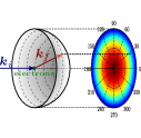
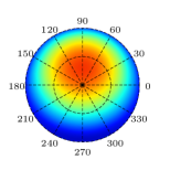
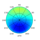
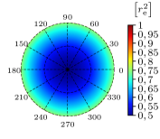
$\Delta m=2$

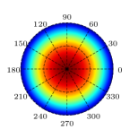
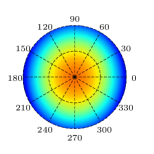
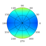
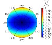
Figure 3: (Color online) Angular differential cross section $\mathrm{d}\sigma_{\mathrm{2tw}}/\mathrm{d}\Omega$ of Compton scattered light for initial photons in a superposition of twisted waves with $\Delta m=1$ (top) and $\Delta m=2$ (bottom) for different cone opening angles $\theta_{k}$, and for $\delta=0$. The disks represent a projection of the forward scattering hemisphere (see the drawing in the top left panel), i.e. the radial axis of the disks represents $\sin\theta$ for scattering angles $0\leq\theta\leq$90\text{\,}\mathrm{\SIUnitSymbolDegree}$$, and the azimuthal axis represents the azimuthal angle $\varphi$ of the scattered photon. For $\theta_{k}=0$ (left column), again, the cross section coincides with the results of an incident plane-wave photon; they are equal for $\Delta m=1$ and $\Delta m=2$ and they are independent of the azimuthal angle $\varphi$.

Figure 3 displays the angular distributions of Compton scattered photons for an incident superposition of two twisted Bessel photons for $\Delta m=1,2$ and for different cone opening angles $\theta_{k}$. Obviously, the interference term depends on the azimuthal angle $\varphi$ of the scattered photon, and not on the scattering angle $\theta$ alone. The disks in Fig. 3 represent a projection of the forward hemisphere of scattered photons, as drawn in the top left panel. The superpositions of twisted photons break the axial symmetry of the initial state. The number of azimuthal modulations of plane-wave states on the momentum cone is just $\Delta m$ and the orientation of that pattern is determined by the relative phase $\delta$, i.e. by the latitude of the state $|\gamma\rangle$ on the Bloch sphere. Changing the value of $\delta$ results in a rotation of the distributions of scattered photons in Fig. 3 with respect to the azimuthal angle $\varphi$.

Let us briefly discuss the angular distribution in the backward-hemisphere, i.e. for scattering angles $\theta\geq$90\text{\,}\mathrm{\SIUnitSymbolDegree}$$. The distributions can be easily read off Eqs. (37) and (45). In particular, for the case $\Delta m=1$ we obtain the relation $\mathrm{d}\sigma_{\mathrm{2tw}}^{(\Delta m=1)}/\mathrm{d}\Omega(\theta,\varphi)=\mathrm{d}\sigma_{\mathrm{2tw}}^{(\Delta m=1)}/\mathrm{d}\Omega(\pi-\theta,-\varphi-2\delta)$. For $\Delta m=2$, on the other hand, we obtain the symmetry relation $\mathrm{d}\sigma_{\mathrm{2tw}}^{(\Delta m=2)}/\mathrm{d}\Omega(\theta,\varphi)=\mathrm{d}\sigma_{\mathrm{2tw}}^{(\Delta m=2)}/\mathrm{d}\Omega(\pi-\theta,\varphi)$.

V Conclusions

In summary, a theoretical study has been performed for the Compton scattered of photons from a Bessel beam on electrons in the rest frame of the electrons. In the long-wavelength limit of the incident radiation and based on the non-relativistic Schrödinger’s equation, the density matrix theory has been used to analyze the angle-differential cross section as function of the scattering angle and for Bessel beams with different cone opening angles and total angular momentum.

Our formulation of the problem in the density matrix formulation explains why the angular distribution and polarization of the scattered photons do not depend on the value of the projection of angular momentum: Because of the symmetry of the system only the those elements of the incident twisted photon density matrix contribute to the reduced density matrix of the scattered photons that are diagonal in the momentum quantum numbers. The angular momentum value appears only via the difference of the vortex phase factors of the plane-wave components of the twisted photon and, therefore, vanishes on the diagonal of the density matrix.

We found completely analytical results for the angular and polarization distribution of Compton scattered photons for the scattering of twisted photons. These distributions are sensitive with regard to the momentum cone opening angle $\theta_{k}$. In particular we observed a depolarization of the scattered radiation for large values of this cone opening angle. In addition, it was found that the angular distributions of the scattered photons for a superpositions of twisted photon beams with different $m$ differ from the case of a single TAM eigenstate if $\Delta m=1$ or $2$ due to dipole selection rules. These differences vanish for $|\Delta m|>2$ in the dipole approximation and remain small if non-dipole contributions are taken into account.

For beams of photons and/or electrons of higher energy, a relativistic treatment of the electron-photon interaction might be more appropriate instead but should not change the central results of this work as long as the changes in the recoil parameter are moderate. In fact, as long as the recoil parameter $r$ in Eq. (1) is small, our results can be directly translated to scenarios of inverse Compton scattering by applying a suitable Lorentz transformation. For inverse Compton scattering, low-frequency photons (e.g. optial laser photons) are scattered on ultra-relativistic electrons, and the backscattered photons’ frequency is Doppler up-shifted to the x-ray regime.

*

Appendix A Normalization of quantum states of plane-wave and twisted photons

In this Appendix we discuss all necessary details on the normalization of the quantum states that enter the calculation of the final-state density matrix in the non-relativistic Compton scattering of plane-wave or twisted light. The usual normalization in a finite box does not work in this case, because the twisted photons are cylindrical symmetric modes. Moreover, the states of twisted photons are represented as a continuous coherent superposition of plane waves, while in a finite-sized box the momentum modes are discrete. Therefore, we need to quantize the modes in an infinite volume $V\to\infty$. In order to correctly normalize twisted-particle quantum states we will explicitly keep all the factors of the formally infinite volume. We normalize all one-particle quantum states $|\psi\rangle$, i.e. for the electrons and the plane-wave or twisted photons, to unity: $\langle\psi\hskip 1.00006pt|\hskip 1.00006pt\psi\rangle=1$. In the following we discuss what this implies in detail for the electron and photon states, their density operators, spatial wavefunctions, as well as for the spatial probability density.

A.1 Plane-wave electron states

Throughout our paper, all initial and final states of the electrons are described as plane waves, i.e. as momentum eigenstates $\hat{\boldsymbol{p}}|p\rangle=\boldsymbol{p}|p\rangle$, where $\hat{\boldsymbol{p}}$ is the electron momentum operator, and the states are characterized by the three quantum numbers of the linear momentum eigenvalue $\boldsymbol{p}=(p_{x},p_{y},p_{z})$. We require that the one-particle states are normalized as

$$\langle\boldsymbol{p}\hskip 1.00006pt|\hskip 1.00006pt\boldsymbol{p}\rangle=1\,,$$ (47)

and, hence, for the orthogonality relation

$$\langle\boldsymbol{p}^{\prime}\hskip 1.00006pt|\hskip 1.00006pt\boldsymbol{p}\rangle=\left(\frac{2\pi}{L}\right)^{3}\delta(\boldsymbol{p}^{\prime}-\boldsymbol{p})\,,$$ (48)

and where the normalization (47) follows from (48) with the usual interpretation of $\lim_{\boldsymbol{p}^{\prime}\to\boldsymbol{p}}\delta(\boldsymbol{p}^{\prime}-\boldsymbol{p})=(L/2\pi)^{3}$ Peskin and Schroeder (1995).

We may define a regularized delta distribution

$$\widetilde{\delta}(\boldsymbol{p}^{\prime}-\boldsymbol{p}):=\left(\frac{2\pi}{L}\right)^{3}\delta(\boldsymbol{p}^{\prime}-\boldsymbol{p})\,,$$ (49)

which has the property $\lim_{\boldsymbol{p}^{\prime}\to\boldsymbol{p}}\widetilde{\delta}(\boldsymbol{p}^{\prime}-\boldsymbol{p})=1$. The properly normalized integration measure for these plane-wave states is given by

$$\int\!\widetilde{\mathrm{d}\boldsymbol{p}}:=\int\!\left(\frac{L}{2\pi}\right)^{3}\mathrm{d}^{3}\boldsymbol{p}\,.$$ (50)

In particular, $\int\!\widetilde{\mathrm{d}\boldsymbol{p}}\,\widetilde{\delta}(\boldsymbol{p}-\boldsymbol{p}^{\prime})=1$. These definitions also provide the correct way of counting the number of final states; their density is just $\widetilde{\mathrm{d}\boldsymbol{p}}$. Moreover, the completeness relation for the plane-wave electron states is

$$\int\!\widetilde{\mathrm{d}\boldsymbol{p}}\,|\boldsymbol{p}\rangle\langle\boldsymbol{p}|=\hat{1}\,.$$ (51)

Because the states $|\boldsymbol{p}\rangle$ are normalized, the trace of the density operator $\hat{\rho}_{\boldsymbol{p}}=|\boldsymbol{p}\rangle\langle\boldsymbol{p}|$ is just unity ${\rm tr}\,(\hat{\rho}_{\boldsymbol{p}})=1$, where we also have to take the integration measure (50) when calculating the trace of the density matrix.

The position space wave function is just given by $\psi_{\boldsymbol{p}}(\boldsymbol{x})=\langle\boldsymbol{x}\hskip 1.00006pt|\hskip 1.00006pt\boldsymbol{p}\rangle=e^{i\boldsymbol{p}\cdot\boldsymbol{x}}/\sqrt{V}$. The particle density is determined as the expectation value of the particle density operator $\hat{n}(\boldsymbol{x})=|\boldsymbol{x}\rangle\langle\boldsymbol{x}|$, as $n_{\boldsymbol{p}}(\boldsymbol{x})={\rm tr}\,\hat{n}(\boldsymbol{x})\hat{\rho}_{\boldsymbol{p}}$ and just yields a constant local particle density of $n_{\boldsymbol{p}}(\boldsymbol{x})=1/V$. Therefore one usually says that the plane-waves (47) are normalized to one particle in the infinite quantization volume $V=L^{3}\to\infty$.

A.2 Plane-wave photon states

We apply the same normalization to the plane-photon states as we employed for the plane-wave electron states in the previous subsection. The only small difference is that the photon states are characterized also by their helicity $\Lambda$ in addition to the linear momentum eigenvalue $\boldsymbol{k}$. We thus orthonormalize the plane-wave one particle photon states $|\boldsymbol{k}\Lambda\rangle$ as

$$\langle\boldsymbol{k}\Lambda\hskip 1.00006pt|\hskip 1.00006pt\boldsymbol{k}^{\prime}\Lambda^{\prime}\rangle=\delta_{\Lambda\Lambda^{\prime}}\widetilde{\delta}(\boldsymbol{k}-\boldsymbol{k}^{\prime})\,.$$ (52)

Moreover, we quantize the photon field, expanding the photon field operator

$$\hat{\boldsymbol{A}}(\boldsymbol{x})=\sumint\limits_{\Lambda}\!\widetilde{\mathrm{d}\boldsymbol{k}}\,N_{k}\left[\hat{c}_{\boldsymbol{k}\Lambda}\boldsymbol{u}_{\boldsymbol{k}\Lambda}(\boldsymbol{x})+\hat{c}_{\boldsymbol{k}\Lambda}^{\dagger}\boldsymbol{u}_{\boldsymbol{k}\Lambda}^{*}(\boldsymbol{x})\right]\,,$$ (53)

into a circularly polarized plane-wave basis $\boldsymbol{u}_{\boldsymbol{k}\Lambda}(\boldsymbol{x})=e^{i\boldsymbol{k}\cdot\boldsymbol{x}}\,\boldsymbol{\varepsilon}_{\boldsymbol{k}\Lambda}$, and with the same meaning of $\widetilde{\mathrm{d}\boldsymbol{k}}$ as for plane-wave electrons. The normalization factor $N_{k}=\sqrt{2\pi c/kV}$ is chosen in such a way that the free Hamiltonian of the photon field is given by

$$H_{\gamma}=\frac{1}{8\pi}\int\!\mathrm{d}^{3}\boldsymbol{x}\,(\hat{\boldsymbol{E}}^{2}+\hat{\boldsymbol{B}}^{2})\\ \stackrel{{\scriptstyle!}}{{=}}\sumint\limits_{\Lambda}\!\widetilde{\mathrm{d}\boldsymbol{k}}\,\omega_{k}\left(\hat{c}_{\boldsymbol{k}\Lambda}^{\dagger}\hat{c}_{\boldsymbol{k}\Lambda}+\frac{1}{2}\right)\,,$$ (54)

where $\hat{\boldsymbol{E}}$ and $\boldsymbol{B}$ are the electric and magnetic field operators, respectively.

The one-particle states are generated by the photon creation operators from the vacuum (zero-photon) state

$$|\boldsymbol{k}\Lambda\rangle=\hat{c}_{\boldsymbol{k}\Lambda}^{\dagger}|0\rangle\,.$$ (55)

The commutation relations of the photon creation and annihilation operators

$$[\hat{c}_{\boldsymbol{k}\Lambda},\hat{c}_{\boldsymbol{k}^{\prime}\Lambda^{\prime}}^{\dagger}]=\delta_{\Lambda\Lambda^{\prime}}\widetilde{\delta}(\boldsymbol{k}-\boldsymbol{k}^{\prime})$$ (56)

completely fix the orthonormalization (52).

The proper measure of the final states now includes a sum over the helicity states, thus, the completeness relation is given by

$$\sumint\limits_{\Lambda}\!\widetilde{\mathrm{d}\boldsymbol{k}}\,|\boldsymbol{k}\Lambda\rangle\langle\boldsymbol{k}\Lambda|=\hat{1}\,.$$ (57)

That means we need to include the sum over the two helicity states in the trace of the photonic density matrix in order have ${\rm tr}\,(\hat{\rho}_{\boldsymbol{k}\Lambda})=1$, and with the same interpretation of having one particle per volume $V$ as above. The vector potential that corresponds to the plane-wave one-photon state can be calculated as

$$\boldsymbol{A}_{\boldsymbol{k}\Lambda}(\boldsymbol{x}):=\langle 0\hskip 1.00006pt|\hskip 1.00006pt\hat{\boldsymbol{A}}(\boldsymbol{x})\hskip 1.00006pt|\hskip 1.00006pt\boldsymbol{k}\Lambda\rangle=N_{k}\boldsymbol{u}_{\boldsymbol{k}\Lambda}\\ =\sqrt{\frac{2\pi c}{kV}}\boldsymbol{\varepsilon}_{\boldsymbol{k}\Lambda}e^{i\boldsymbol{k}\cdot\boldsymbol{x}}\,.$$ (58)

A.3 Twisted-wave photon states

Twisted photons are cylindrical symmetric modes and therefore need to be normalized to a cylindrical volume $V=\pi R^{2}L_{z}$ with radius $R$ and height $L_{z}$ along the $z$-axis. The twisted photon states that we defined in Eq. (28) are orthonormalized in the following sense:

$$\langle\kappa_{\perp}^{\prime}\kappa_{\parallel}^{\prime}m^{\prime}\Lambda^{\prime}\hskip 1.00006pt|\hskip 1.00006pt\kappa_{\perp}\kappa_{\parallel}m\Lambda\rangle\\ =\frac{2\pi^{2}}{RL_{z}}\delta(\kappa_{\parallel}^{\prime}-\kappa_{\parallel})\delta(\kappa_{\perp}^{\prime}-\kappa_{\perp})\delta_{m^{\prime}m}\delta_{\Lambda^{\prime}\Lambda}\,,$$ (59)

which implies that $\langle\kappa_{\perp}\kappa_{\parallel}m\Lambda\hskip 1.00006pt|\hskip 1.00006pt\kappa_{\perp}\kappa_{\parallel}m\Lambda\rangle=1$. To prove this normalization we make use of the identity for the radial delta function

$$\lim_{\kappa_{\perp}^{\prime}\to\kappa_{\perp}}\delta(\kappa_{\perp}^{\prime}-\kappa_{\perp})=\frac{R}{\pi}\,,$$ (60)

where $R$ is the (infinite) radius of the cylindrical normalization volume. The above identification was proven, e.g., in Refs. Jentschura and Serbo (2011b); Ivanov (2011). Moreover, for the longitudinal momentum delta function we employ the usual relation $\delta(\kappa_{\parallel}=0)=L_{z}/2\pi$, where $L_{z}$ is the height of the quantization cylinder.

The probability density that can be attributed to the twisted one-particle states $n_{\kappa_{\perp}\kappa_{\parallel}m\Lambda}(\boldsymbol{x})={\rm tr}\,(\hat{n}(\boldsymbol{x})\hat{\rho}_{\kappa_{\perp}\kappa_{\parallel}m\Lambda})$ turns out the be not spatially constant, but instead is given by

$$n_{\kappa_{\perp}\kappa_{\parallel}m\Lambda}(\boldsymbol{x}) =\frac{\kappa_{\perp}}{2L_{z}R}J_{m}^{2}(\kappa_{\perp}x_{\perp})\,,$$ (61)

where $J_{m}$ are the Bessel functions of the first kind Watson (1922).

The spatially averaged probability density

$$\langle n\rangle:=\frac{1}{V}\!\int\!\mathrm{d}^{3}\boldsymbol{x}\,n(\boldsymbol{x})=\frac{1}{V}\,{\rm tr}\hat{\rho}$$ (62)

which enters the definition of the cross section, Eq. (6), is just proportional to the trace of the density operator because the position eigenstates form a complete basis. That means, also for twisted photons a normalized density operator correspond to one particle per volume $V=\pi L_{z}R^{2}$. The spatially averaged probability density can also be calculated directly from Eq. (61) as

$$\langle n_{\kappa_{\perp}\kappa_{\parallel}m\Lambda}\rangle =\frac{1}{V}\!\int\!\mathrm{d}\varphi\,\mathrm{d}z\,\mathrm{d}x_{\perp}\,x_{\perp}\frac{\kappa_{\perp}}{2L_{z}R}J_{m}^{2}(\kappa_{\perp}x_{\perp})$$

$$=\frac{1}{V}\frac{\pi}{R}\!\int\limits_{0}^{R}\!\mathrm{d}x_{\perp}\,x_{\perp}\kappa_{\perp}\,J_{m}^{2}(\kappa_{\perp}x_{\perp})\,,$$ (63)

and by approximating the radial integral over $x_{\perp}$ for large $R\to\infty$ by using the asymptotic expansion of the Bessel function for large arguments, $J_{m}(x)\approx\sqrt{2/\pi x}\,\cos(x-m\pi/2-\pi/4)$ Watson (1922); Jentschura and Serbo (2011b), yielding

$$\int\limits_{0}^{R}\mathrm{d}x_{\perp}\,\kappa_{\perp}x_{\perp}\,J_{m}^{2}(\kappa_{\perp}x_{\perp})\approx\frac{R}{\pi}\,.$$ (64)

The vector potential that corresponds to the twisted one-photon states is given by

$$\boldsymbol{A}_{\kappa_{\perp}\kappa_{\parallel}m\Lambda}(\boldsymbol{x})=\langle 0\hskip 1.00006pt|\hskip 1.00006pt\hat{\boldsymbol{A}}(\boldsymbol{x})\hskip 1.00006pt|\hskip 1.00006pt\kappa_{\perp}\kappa_{\parallel}m\Lambda\rangle\\ =\sqrt{\frac{2\pi^{2}c^{2}}{\omega L_{z}R}}\int\!\frac{\mathrm{d}^{2}\boldsymbol{k}_{\perp}}{(2\pi)^{2}}a_{\kappa_{\perp}m}(\boldsymbol{k}_{\perp})\boldsymbol{\varepsilon}_{\boldsymbol{k}\Lambda}e^{i\boldsymbol{k}_{\perp}\cdot\boldsymbol{x}_{\perp}+i\kappa_{\parallel}z}\,.$$ (65)

Except for the different normalization factor in front of the integral, this coincides with the vector potential employed in Ref. Matula et al. (2013) to define the twisted light. It was argued in Matula et al. (2013) that $A^{\mu}_{\kappa_{\perp}\kappa_{\parallel}m\Lambda}(\boldsymbol{x})$ describes a beam with well-defined projection of total angular momentum $m$. The product of the amplitude $a_{\kappa_{\perp}m}(\boldsymbol{k}_{\perp})$ and the plane-wave polarization vector $\boldsymbol{\varepsilon}_{\boldsymbol{k}\Lambda}$ was shown to be an eigenfunction of the $z$-component of the total angular momentum operator $\hat{J}_{z}$ with the eigenvalue $m$.

Performing the momentum integrations in the above Fourier integral we obtain for the twisted-wave vector potential

$$\boldsymbol{A}_{\kappa_{\perp}\kappa_{\parallel}m\Lambda}(\boldsymbol{x})=\sqrt{\frac{2\pi^{2}c^{2}}{\omega L_{z}R}}\sqrt{\frac{\kappa_{\perp}}{2\pi}}\,e^{i\kappa_{\parallel}z}\\ \times\sum_{m=0,\pm 1}(-1)^{m_{s}}c_{m_{s}}(\Lambda)J_{m-m_{s}}(\kappa_{\perp}x_{\perp})e^{i(m-m_{s})\varphi}\boldsymbol{\eta}_{m_{s}}$$ (66)

where the sum over $m_{s}$ runs over all possible projections of the photon spin angular momentum onto the $z$-direction and accounts for the coupling of (the projections of) orbital angular momentum ($m_{\ell}$) and spin angular momentum ($m_{s}$) to the total angular momentum $m=m_{\ell}+m_{s}$. This representation of the twisted wave vector potential employs the unit vectors $\boldsymbol{\eta}_{0}=(0,0,1)^{T}$ and $\boldsymbol{\eta}_{\pm 1}=(1,\pm i,0)^{T}/\sqrt{2}$, and the coefficients $c_{0}=-\frac{1}{\sqrt{2}}\sin\theta_{k}$ and $c_{\pm 1}=\frac{1}{2}(1\pm\Lambda\cos\theta_{k})$ with the momentum cone opening angle $\tan\theta_{k}=\kappa_{\perp}/\kappa_{\parallel}$.

References

- Compton (1923) A. H. Compton, “A quantum theory of the scattering of x-rays by light elements,” Phys. Rev. 21, 483 (1923).
- Klein and Nishina (1929) O. Klein and Y. Nishina, “Über die Streuung von Strahlung durch freie Elektronen nach der neuen relativistischen Quantenmechanik nach Dirac,” Z. Phys. 52, 853 (1929).
- Jackson (1983) J. D. Jackson, Klassische Elektrodynamik, 2nd ed. (Walter de Gruyter, Berlin, New York, 1983).
- Greiner (1989) W. Greiner, Quantentheorie: Spezielle Kapitel, 3rd ed., Theoretische Physik, Vol. 4A (Verlag Harri Deutsch, 1989).
- Berestetzki et al. (1980) W. B. Berestetzki, E. M. Lifschitz, and L. P. Pitajewski, Relativistische Quantentheorie, Lehrbuch der Theoretischen Physik, Vol. IV (Akademie Verlag, Berlin, 1980).
- Allen et al. (1992) L. Allen, M. W. Beijersbergen, R. J. C. Spreeuw, and J. P. Woerdman, “Orbital angular momentum of light and the transformation of Laguerre-Gaussian laser modes,” Phys. Rev. A 45, 8185 (1992).
- O’Neil et al. (2002) A. T. O’Neil, I. MacVicar, L. Allen, and M. Padgett, “Intrinsic and extrinsic nature of the orbital angular momentum of a light beam,” Phys. Rev. Lett. 88, 053601 (2002).
- Molina-Terriza et al. (2007) G. Molina-Terriza, J. P. Torres, and L. Torner, “Twisted photons,” Nature Phys. 3, 305 (2007).
- Yao and Padgett (2011) A. M. Yao and M. J. Padgett, “Orbital angular momentum: origins, behavior and applications,” Advances in Optics and Photonics 3, 161 (2011).
- Andrews and Babiker (2013) D. L. Andrews and M. Babiker, eds., The Angular Momentum of Light (Cambridge University Press, 2013).
- Blum (2012) K. Blum, Density Matrix Theory and Applications, 3rd ed., Springer Series on Atomic, Optical, and Plasma Physics, Vol. 64 (Springer-Verlag, Berlin, Heidelberg, New York, 2012).
- Englert and Rinehart (1983) T. J. Englert and E. A. Rinehart, “Second-harmonic photons from the interaction of free electrons with intense laser radiation,” Phys. Rev. A 28, 1539 (1983).
- Cojoc et al. (2006) D. Cojoc, B. Kaulich, A. Carpentiero, S. Cabrini, L. Businaro, and E. Di Fabrizio, “X-ray vortices with high topological charge,” Microelectronic Engineering 83, 1360 (2006).
- Zürch et al. (2012) M. Zürch, C. Kern, P. Hansinger, A. Dreischuh, and Ch. Spielmann, “Strong-field physics with singular light beams,” Nature Phys. 8, 743 (2012).
- Hemsing et al. (2013) E. Hemsing, A. Knyazik, M. Dunning, D. Xiang, A. Marinelli, C. Hast, and J. B. Rosenzweig, “Coherent optical vortices from relativistic electron beams,” Nature Phys. 9, 549 (2013).
- Bahrdt et al. (2013) J. Bahrdt, K. Holldack, P. Kuske, R. Müller, M. Scheer, and P. Schmid, “First observation of photons carrying orbital angular momentum in undulator radiation,” Phys. Rev. Lett. 111, 034801 (2013).
- Gariepy et al. (2014) G. Gariepy, J. Leach, K. T. Kim, T. J. Hammond, E. Frumker, R. W. Boyd, and P. B. Corkum, “Creating high-harmonic beams with controlled orbital angular momentum,” Phys. Rev. Lett. 113, 153901 (2014).
- Arlt and Dholakia (2000) J. Arlt and K. Dholakia, “Generation of high-order bessel beams by use of an axicon,” Opt. Commun. 177, 297 (2000).
- Kumar et al. (2010) A. Kumar, P. Vaity, Y. Krishna, and R. P. Singh, “Engineering the size of dark core of an optical vortex,” Opt. Las. in Engineering 48, 276 (2010).
- Balashov et al. (2000) V. V. Balashov, A. N. Grum-Grzhimailo, and N. M. Kabachnik, Polarization and Correlation Phenomena in Atomic Collisions (Springer, 2000).
- Surzhykov et al. (2015) A. Surzhykov, D. Seipt, V. G. Serbo, and S. Fritzsche, “Interaction of twisted light with many-electron atoms and ions,” Phys. Rev. A 91, 013403 (2015).
- Taylor (1972) J. R. Taylor, Scattering Theory: The Quantum Theory of Nonrelativistic Collisions (John Wiley & Sons, 1972).
- Landau and Lifschitz (1992) L. D. Landau and E. M. Lifschitz, Klassische Feldtheorie, 12th ed., Lehrbuch der Theoretischen Physik, Vol. 2 (Akademie Verlag, 1992).
- Note (1) By using the relation for the energy delta function in the limit Peskin and Schroeder (1995).
- Noether (1918) E. Noether, “Invariante Variationsprobleme,” Nachr. Ges. Wiss. Göttingen, Math.-Phys. Kl. 1918, 235–257 (1918), english translation: M. A. Travel, Transport Theory and Statistical Physics 1, 183 (1971).
- McMaster (1961) W. H. McMaster, “Matrix representation of polarization,” Rev. Mod. Phys. 33, 8 (1961).
- Matula et al. (2013) O. Matula, A. G. Hayrapetyan, V. G. Serbo, A. Surzhykov, and S. Fritzsche, “Atomic ionization of hydrogen-like ions by twisted photons: angular distribution of emitted electrons,” J. Phys. B 46, 205002 (2013).
- Jentschura and Serbo (2011a) U. D. Jentschura and V. G. Serbo, “Generation of high-energy photons with large orbital angular momentum by Compton backscattering,” Phys. Rev. Lett. 106, 013001 (2011a).
- Ivanov (2011) I. P. Ivanov, “Colliding particles carrying nonzero orbital angular momentum,” Phys. Rev. D 83, 093001 (2011).
- Seipt et al. (2014) D. Seipt, A. Surzhykov, and S. Fritzsche, “Structured x-ray beams from twisted electrons by inverse Compton scattering of laser light,” Phys. Rev. A 90, 012118 (2014).
- Scholz-Marggraf et al. (2014) H. M. Scholz-Marggraf, S. Fritzsche, V. G. Serbo, A. Afanasev, and A. Surzhykov, “Absorption of twisted light by hydrogenlike atoms,” Phys. Rev. A 90, 013425 (2014).
- Note (2) V. G. Serbo, I. V. Ivanov, S. Fritzsche, D. Seipt, and A. Surzhykov, “Scattering of twisted relativistic electrons by atoms”, submitted.
- Ivanov (2012) I. P. Ivanov, “Measuring the phase of the scattering amplitude with vortex beams,” Phys. Rev. D 85, 076001 (2012).
- Lloyd et al. (2012) S. Lloyd, M. Babiker, and J. Yuan, “Quantized orbital angular momentum transfer and magnetic dichroism in the interaction of electron vortices with matter,” Phys. Rev. Lett. 108, 074802 (2012).
- Van Boxem et al. (2014) R. Van Boxem, B. Partoens, and J. Verbeeck, “Rutherford scattering of electron vortices,” Phys. Rev. A 89, 032715 (2014).
- Van Boxem et al. (2015) R. Van Boxem, B. Partoens, and J. Verbeeck, “Inelastic electron-vortex-beam scattering,” Phys. Rev. A 91, 032703 (2015).
- Quinteiro et al. (2015) G. F. Quinteiro, D. E. Reiter, and T. Kuhn, “Formulation of the twisted-light–matter interaction at the phase singularity: The twisted-light gauge,” Phys. Rev. A 91, 033808 (2015).
- Jentschura and Serbo (2011b) U. D. Jentschura and V. G. Serbo, “Compton upconversion of twisted photons: backscattering of particles with non-planar wave functions,” Eur. Phys. J. C 71, 1571 (2011b).
- Vasilyeu et al. (2009) R. Vasilyeu, A. Dudley, N. Khilo, and A. Forbes, “Generating superpositions of higher–order bessel beams,” Opt. Express 17, 23389 (2009).
- Peskin and Schroeder (1995) M. E. Peskin and D. V. Schroeder, An Introduction to Quantum Field Theory (Addison-Wesley Publishing Company, 1995).
- Watson (1922) G. N. Watson, A treatise on the theory of Bessel functions (Cambridge University Press, 1922).