Algorithms for Lipschitz Learning on Graphs

Abstract

We develop fast algorithms for solving regression problems on graphs where one is given the value of a function at some vertices, and must find its smoothest possible extension to all vertices. The extension we compute is the absolutely minimal Lipschitz extension, and is the limit for large $p$ of $p$-Laplacian regularization. We present an algorithm that computes a minimal Lipschitz extension in expected linear time, and an algorithm that computes an absolutely minimal Lipschitz extension in expected time $\widetilde{O}(mn)$. The latter algorithm has variants that seem to run much faster in practice. These extensions are particularly amenable to regularization: we can perform $l_{0}$-regularization on the given values in polynomial time and $l_{1}$-regularization on the initial function values and on graph edge weights in time $\widetilde{O}(m^{3/2})$.

Our definitions and algorithms naturally extend to directed graphs.

1 Introduction

We consider a problem in which we are given a weighted undirected graph $G=(V,E,\ell)$ and values $v_{0}\mathrel{\mathop{\mathchar 58\relax}}T\to\mathbb{R}$ on a subset $T$ of its vertices. We view the weights $\ell$ as indicating the lengths of edges, with shorter length indicating greater similarity. Our goal it to assign values to every vertex $v\in V\backslash T$ so that the values assigned are as smooth as possible across edges. A minimal Lipschitz extension of $v_{0}$ is a vector $v$ that minimizes

$$\max_{(x,y)\in E}(\ell{(x,y)})^{-1}\left|v(x)-v(y)\right|,$$ (1)

subject to $v(x)=v_{0}(x)$ for all $x\in T$. We call such a vector an inf-minimizer. Inf-minimizers are not unique. So, among inf-minimizers we seek vectors that minimize the second-largest absolute value of $\ell{(x,y)}^{-1}\left|v(x)-v(y)\right|$ across edges, and then the third-largest given that, and so on. We call such a vector $v$ a lex-minimizer. It is also known as an absolutely minimal Lipschitz extension of $v_{0}$.

These are the limit of the solution to $p$-Laplacian minimization problems for large $p$, namely the vectors that solve

$$\min_{\begin{subarray}{c}v\in\mathbb{R}^{n}\\ v|_{T}=v_{0}|_{T}\end{subarray}}\sum_{(x,y)\in E}(\ell{(x,y)})^{-p}|v(x)-v(y)|^{p}.$$ (2)

The use of $p=2$ was suggested in the foundational paper of Zhu et al. (2003), and is particularly nice because it can be obtained by solving a system of linear equations in a symmetric diagonally dominant matrix, which can be done very quickly (Cohen et al. (2014)). The use of larger values of $p$ has been discussed by Alamgir and Luxburg (2011), and by Bridle and Zhu (2013), but it is much more complicated to compute. The fastest algorithms we know for this problem require convex programming, and then require very high accuracy to obtain the values at most vertices. By taking the limit as $p$ goes to infinity, we recover the lex-minimizer, which we will show can be computed quickly.

The lex-minimization problem has a remarkable amount of structure. For example, in uniformly weighted graphs the value of the lex-minimizer at every vertex not in $T$ is equal to the average of the minimum and maximum of the values at its neighbors. This is analogous to the property of the $2$-Laplacian minimizer that the value at every vertex not in $T$ equals the average of the values at its neighbors.

1.1 Contributions

We first present several important structural properties of lex-minimizers in Section 3.2. As we shall point out, some of these were known from previous work, sometimes in restricted settings. We state them generally and prove them for completeness. We also prove that the lex-minimizer is as stable as possible under perturbations of $v_{0}$ (Section 3.1).

The structure of the lex-minimization problem has led us to develop elegant algorithms for its solution. Both the algorithms and their analyses could be taught to undergraduates. We believe that these algorithms could be used in place of $2$-Laplacian minimization in many applications.

We present algorithms for the following problems. Throughout, $m=\left|E\right|$ and $n=\left|V\right|$.

Inf-minimization:

An algorithm that runs in expected time $O(m+n\log n)$ (Section 4.3).

Lex-minimization:

An algorithm that runs in expected time $O(n(m+n\log n))$ (Section 4), along with a variant that runs quickly in practice (Section 4.4).

$l_{1}$-regularization of edge lengths for inf-minimization:

The problem of minimizing (1) given a limited budget with which one can increase edge lengths is a linear programming problem. We show how to solve it in time $\widetilde{O}(m^{3/2})$ with an interior point method by using fast Laplacian solvers (Section 8). The same algorithm can accommodate $l_{1}$-regularization of the values given in $v_{0}$.

$l_{0}$-regularization of vertex values for inf-minimization:

We give a polynomial time algorithm for $l_{0}$-regularization of the values at vertices. That is, we minimize (1) given a budget of a number of vertices that can be proclaimed outliers and removed from $T$ (Section 7.1). We solve this problem by reducing it to the problem of computing minimum vertex covers on transitively closed directed acyclic graphs, a special case of minimum vertex cover that can be solved in polynomial time.

After any regularization for inf-minimization, we suggest computing the lex-minimizer. We find the result for $l_{0}$-regularization of vertex values to be particularly surprising, especially because we prove that the analogous problem for $2$-Laplacian minimization is NP-Hard (Section 7.2).

All of our algorithms extend naturally to directed graphs (Section 5). This is in contrast with the problem of minimizing $2$-Laplacians on directed graphs, which corresponds to computing electrical flows in networks of resistors and diodes, for which fast algorithms are not presently known.

We present a few experiments on examples demonstrating that the lex-minimizer can overcome known deficiencies of the $2$-Laplacian minimizer (Section 1.2, Figures 1,2), as well as a demonstration of the performance of the directed analog of our algorithms on the WebSpam dataset of Castillo et al. (2006) (Section 6). In the WebSpam problem we use the link structure of a collection of web sites to flag some sites as spam, given a small number of labeled sites known to be spam or normal.

1.2 Relation to Prior Work

We first encountered the idea of using the minimizer of the 2-Laplacian given by (2) for regression and classification on graphs in the work of Zhu et al. (2003) and Belkin et al. (2004) on semi-supervised learning. These works transformed learning problems on sets of vectors into problems on graphs by identifying vectors with vertices and constructing graphs with edges between nearby vectors. One shortcoming of this approach (see Nadler et al. (2009), Alamgir and Luxburg (2011), Bridle and Zhu (2013)) is that if the number of vectors grows while the number of labeled vectors remains fixed, then almost all the values of the 2-Laplacian minimizer converge to the mean of the labels on most natural examples. For example, Nadler et al. (2009) consider sampling points from two Gaussian distributions centered at $0$ and $4$ on the real line. They place edges between every pair of points $(x,y)$ with length $\exp(\left|x-y\right|^{2}/2\sigma^{2})$ for $\sigma=0.4$, and provide only the labels $v_{0}(0)=-1$ and $v_{0}(4)=1$. Figure 1 shows the values of the $2$-Laplacian minimizer in red, which are all approximately zero. In contrast, the values of the lex-minimizer in blue, which are smoothly distributed between the labeled points, are shown.

The “manifold hypothesis” (see Chapelle et al. (2010), Ma and Fu (2011)) holds that much natural data lies near a low-dimensional manifold and that natural functions we would like to learn on this data are smooth functions on the manifold. Under this assumption, one should expect lex-minimizers to interpolate well. In contrast, the $2$-Laplacian minimizers degrade (dotted lines) if the number of labeled points remains fixed while the total number of points grows. In Figure 2, we demonstrate this by sampling many points uniformly from the unit cube in 4 dimensions, form their 8-nearest neighbor graph, and consider the problem of regressing the first coordinate. We performed 8 experiments, varying the number of labeled points in $\left\{50,100,500,1000\right\}$. Each data point is the mean average $l_{1}$ error over 100 experiments. The plots for root mean squared error are similar. The standard deviation of the estimations of the mean are within one pixel, and so are not displayed. The performance of the lex-minimizer (solid lines) does not degrade as the number of unlabeled points grows.

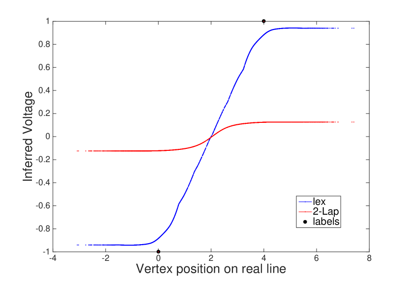
Figure 1: Lex vs 2-Laplacian on 1D gaussian clusters.

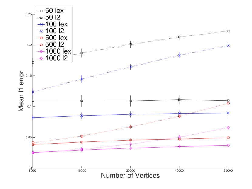
Figure 2: kNN graphs on samples from 4D cube.

Analogous to our inf-minimizers, minimal Lipschitz extensions of functions in Euclidean space and over more general metric spaces have been studied extensively in Mathematics (Kirszbraun (1934), McShane (1934), Whitney (1934)). von Luxburg and Bousquet (2003) employ Lipschitz extensions on metric spaces for classification and relate these to Support Vector Machines. Their work inspired improvements in classification and regression in metric spaces with low doubling dimension (Gottlieb et al. (2013), Gottlieb et al. (2013b)). Theoretically fast, although not actually practical, algorithms have been given for constructing minimal Lipschitz extensions of functions on low-dimensional Euclidean spaces (Fefferman (2009a), Fefferman and Klartag (2009), Fefferman (2009b)). Sinop and Grady (2007) suggest using inf-minimizers for binary classification problems on graphs. For this special case, where all of the given values are either 0 or 1, they present an $O(m+n\log n)$ time algorithm for computing an inf-minimizer. The case of general given values, which we solve in this paper, is much more complicated. To compensate for the non-uniqueness of inf-minimizers, they suggest choosing the inf-minimizer that minimizes (2) with $p=2$. We believe that the lex-minimizer is a more natural choice.

The analog of our lex-minimizer over continuous spaces is called the absolutely minimal Lipschitz extension (AMLE). Starting with the work of Aronsson (1967), there have been several characterizations and proofs of the existence and uniqueness of the AMLE (Jensen (1993), Crandall et al. (2001), Barles and Busca (2001), Aronsson et al. (2004)). Many of these results were later extended to general metric spaces, including graphs (Milman (1999), Peres et al. (2011), Naor and Sheffield (2010), Sheffield and Smart (2010)). However, to the best of our knowledge, fast algorithms for computing lex-minimizers on graphs were not known. For the special case of undirected, unweighted graphs, Lazarus et al. (1999) presented both a polynomial-time algorithm and an iterative method. Oberman (2011) suggested computing the AMLE in Euclidean space by first discretizing the problem and then solving the corresponding graph problem by an iterative method. However, no run-time guarantees were obtained for either iterative method.

2 Notation and Basic Definitions

Lexicographic Ordering.

Given a vector $r\in\mathbb{R}^{m},$ let $\pi_{r}$ denote a permutation that sorts $r$ in non-increasing order by absolute value, i.e., $\forall i\in[m-1],|r(\pi_{r}(i))|\geq|r(\pi_{r}(i+1))|.$ Given two vectors $r,s\in\mathbb{R}^{m},$ we write $r\preceq s$ to indicate that $r$ is smaller than $s$ in the lexicographic ordering on sorted absolute values, i.e.

$$\exists j\in[m],\left|r(\pi_{r}(j))\right|<\left|s(\pi_{s}(j))\right|\text{ and }\forall i\in[j-1],\left|r(\pi_{r}(i))\right|=\left|s(\pi_{s}(i))\right|$$

or $$\forall i\in[m],\left|r(\pi_{r}(i))\right|=\left|s(\pi_{s}(i))\right|.$$

Note that it is possible that $r\preceq s$ and $s\preceq r$ while $r\neq s$. It is a total relation: for every $r$ and $s$ at least one of $r\preceq s$ or $s\preceq r$ is true.

Graphs and Matrices.

We will work with weighted graphs. Unless explicitly stated, we will assume that they are undirected. For a graph $G$, we let $V_{G}$ be its set of vertices, $E_{G}$ be its set of edges, and $\ell_{G}\mathrel{\mathop{\mathchar 58\relax}}E_{G}\to\mathbb{R}_{+}$ be the assignment of positive lengths to the edges. We let $|V_{G}|=n,$ and $|E_{G}|=m.$ We assume $\ell_{G}$ is symmetric, i.e., $\ell_{G}(x,y)=\ell_{G}(y,x).$ When $G$ is clear from the context, we drop the subscript.

A path $P$ in $G$ is an ordered sequence of (not necessarily distinct) vertices $P=(x_{0},x_{1},\ldots,x_{k}),$ such that $(x_{i-1},x_{i})\in E$ for $i\in[k].$ The endpoints of $P$ are denoted by $\partial_{0}P=x_{0},\partial_{1}P=x_{k}.$ The set of interior vertices of $P$ is defined to be $\operatorname{int}(P)=\{x_{i}\mathrel{\mathop{\mathchar 58\relax}}0<i<k\}.$ For $0\leq i<j\leq k,$ we use the notation $P[x_{i}\mathrel{\mathop{\mathchar 58\relax}}x_{j}]$ to denote the subpath $(x_{i},\ldots,x_{j}).$ The length of $P$ is $\ell(P)=\sum_{i=1}^{k}\ell(x_{i-1},x_{i}).$

A function $v_{0}\mathrel{\mathop{\mathchar 58\relax}}V\to\mathbb{R}\cup\{*\}$ is called a voltage assignment (to $G$). A vertex $x\in V$ is a terminal with respect to $v_{0}$ iff $v_{0}(x)\neq*.$ The other vertices, for which $v_{0}(x)=*$, are non-terminals. We let $T(v_{0})$ denote the set of terminals with respect to $v_{0}.$ If $T(v_{0})=V,$ we call $v_{0}$ a complete voltage assignment (to $G$). We say that an assignment $v\mathrel{\mathop{\mathchar 58\relax}}V\to\mathbb{R}\cup\{*\}$ extends $v_{0}$ if $v(x)=v_{0}(x)$ for all $x$ such that $v_{0}(x)\neq*$.

Given an assignment $v_{0}\mathrel{\mathop{\mathchar 58\relax}}V\to\mathbb{R}\cup\{*\}$, and two terminals $x,y\in T(v_{0})$ for which $(x,y)\in E$, we define the gradient on $(x,y)$ due to $v_{0}$ to be

$$\vspace{-6pt}\mathsf{grad}_{G}[v_{0}](x,y)=\left.\frac{v_{0}(x)-v_{0}(y)}{\ell(x,y)}\right..$$

It may be useful to view $\mathsf{grad}_{G}[v_{0}](x,y)$ as the current in the edge $(x,y)$ induced by voltages $v_{0}$. When $v_{0}$ is a complete voltage assignment, we interpret $\mathsf{grad}_{G}[v_{0}]$ as a vector in $\mathbb{R}^{m},$ with one entry for each edge. However, for convenience, we define $\mathsf{grad}_{G}[v_{0}](x,y)=-\mathsf{grad}_{G}[v_{0}](y,x).$ When $G$ is clear from the context, we drop the subscript.

A graph $G$ along with a voltage assignment $v$ to $G$ is called a partially-labeled graph, denoted $(G,v).$ We say that a partially-labeled graph $(G,v_{0})$ is a well-posed instance if for every maximal connected component $H$ of $G,$ we have $T(v_{0})\cap V_{H}\neq\emptyset.$

A path $P$ in a partially-labeled graph $(G,v_{0})$ is called a terminal path if both endpoints are terminals. We define $\nabla P(v_{0})$ to be its gradient:

$$\vspace{-6pt}\nabla P(v_{0})=\left.\frac{v_{0}(\partial_{0}P)-v_{0}(\partial_{1}P)}{\ell(P)}\right..$$

If $P$ contains no terminal-terminal edges (and hence, contains at least one non-terminal), it is a free terminal path.

Lex-Minimization.

An instance of the Lex-Minimization problem is described by a partially-labeled graph $(G,v_{0}).$ The objective is to compute a complete voltage assignment $v\mathrel{\mathop{\mathchar 58\relax}}V_{G}\to\mathbb{R}$ extending $v_{0}$ that lex-minimizes $\mathsf{grad}[v].$

Definition 2.1 (Lex-minimizer)

Given a partially-labeled graph $(G,v_{0}),$ we define $\mathsf{lex}_{G}[v_{0}]$ to be a complete voltage assignment to $V$ that extends $v_{0},$ and such that for every other complete assignment $v^{\prime}\mathrel{\mathop{\mathchar 58\relax}}V_{G}\to\mathbb{R}$ that extends $v_{0},$ we have $\mathsf{grad}_{G}[\mathsf{lex}_{G}[v_{0}]]\preceq\mathsf{grad}_{G}[v^{\prime}].$ That is, $\mathsf{lex}_{G}[v_{0}]$ achieves a lexicographically-minimal gradient assignment to the edges.

We call $\mathsf{lex}_{G}[v_{0}]$ the lex-minimizer for $(G,v_{0})$. Note that if $T(v_{0})=V_{G},$ then trivially, $\mathsf{lex}_{G}[v_{0}]=v_{0}.$

3 Basic Properties of Lex-Minimizers

Lazarus et al. (1999) established that lex-minimizers in unweighted and undirected graphs exist, are unique, and may be computed by an elementary meta-algorithm. We state and prove these facts for undirected weighted graphs, and defer the discussion of the directed case to Section 5. We also state for directed and weighted graphs characterizations of lex-minimizers that were established by Peres et al. (2011), Naor and Sheffield (2010) and Sheffield and Smart (2010) for unweighted graphs. These results are essential for the analyses of our algorithms. We defer most proofs to Appendix A.

Definition 3.1

A steepest fixable path in an instance $(G,v_{0})$ is a free terminal path $P$ that has the largest gradient $\nabla P(v_{0})$ amongst such paths.

Observe that a steepest fixable path with $\nabla P(v_{0})\neq 0$ must be a simple path.

Definition 3.2

Given a steepest fixable path $P$ in an instance $(G,v_{0}),$ we define $\mathsf{fix}_{G}[v_{0},P]\mathrel{\mathop{\mathchar 58\relax}}V_{G}\to\mathbb{R}\cup\{*\}$ to be the voltage assignment defined as follows

$$\mathsf{fix}_{G}[v_{0},P](x)=\begin{cases}v_{0}(\partial_{0}P)-\nabla P(v_{0})\cdot\ell_{G}(P[\partial_{0}P\mathrel{\mathop{\mathchar 58\relax}}x])&x\in\operatorname{int}(P)\setminus T(v_{0}),\\ v_{0}(x)&\text{otherwise.}\end{cases}$$

We say that the vertices $x\in\operatorname{int}(P)$ are fixed by the operation $\mathsf{fix}[v_{0},P].$ If we define $v_{1}=\mathsf{fix}_{G}[v_{0},P],$ where $P=(x_{0},\ldots,x_{r})$ is the steepest fixable path in $(G,v_{0}),$ then it is easy to argue that for every $i\in[r],$ we have $\mathsf{grad}[v_{1}](x_{i-1},x_{i})=\nabla P$ (see Lemma A.5). The meta-algorithm Meta-Lex, spelled out as Algorithm 1, entails repeatedly fixing steepest fixable paths. While it is possible to have multiple steepest fixable paths, the result of fixing all of them does not depend on the order in which they are fixed.

Theorem 3.3

Given a well-posed instance $(G,v_{0})$, the meta-algorithm Meta-Lex, which repeatedly fixes steepest fixable paths, produces the unique lex-minimizer extending $v_{0}$.

Corollary 3.4

Given a well-posed instance $(G,v_{0})$ such that $T(v_{0})\neq V_{G},$ let $P$ be a steepest fixable path in $(G,v_{0}).$ Then, $(G,\mathsf{fix}[v_{0},P])$ is also a well-posed instance, and $\mathsf{lex}_{G}[\mathsf{fix}[v_{0},P]]=\mathsf{lex}_{G}[v_{0}].$

Since a lex-minimal element must be an inf-minimizer, we also obtain the following corollary, that can also be proved using LP duality.

Lemma 3.5

Suppose we have a well-posed instance $(G,v_{0}).$ Then, there exists a complete voltage assignment $v$ extending $v_{0}$ such that $\left\|\mathsf{grad}[v]\right\|_{\infty}\leq\alpha$, iff every terminal path $P$ in $(G,v_{0})$ satisfies $\nabla P(v_{0})\leq\alpha.$

3.1 Stability

The following theorem states that $\mathsf{lex}_{G}[v_{0}]$ is monotonic with respect to $v_{0}$ and it respects scaling and translation of $v_{0}$.

Theorem 3.6

Let $(G,v_{0})$ be a well-posed instance with $T\mathrel{\mathop{\mathchar 58\relax}}=T(v_{0})$ as the set of terminals. Then the following statements hold.

1. For any $c,d\in\mathbb{R}$, $v_{1}$ a partial assignment with terminals $T(v_{1})=T$ and $v_{1}(t)=cv_{0}(t)+d$ for all $t\in T$. Then, $\mathsf{lex}_{G}[v_{1}](i)=c\cdot\mathsf{lex}_{G}[v_{0}](i)+d$ for all $i\in V_{G}$.

2. $v_{1}$ a partial assignment with terminals $T(v_{1})=T.$ Suppose further that $v_{1}(t)\geq v_{0}(t)$ for all $t\in T.$ Then, $\mathsf{lex}_{G}[v_{1}](i)\geq\mathsf{lex}_{G}[v_{0}](i)$ for all $i\in V_{G}$.

As a corollary, the above theorem gives a nice stability property that lex-minimal elements satisfy.

Corollary 3.7

Given well-posed instances $(G,v_{0})$, $(G,v_{1})$ such that $T\mathrel{\mathop{\mathchar 58\relax}}=T(v_{0})=T(v_{1})$, let $\epsilon\mathrel{\mathop{\mathchar 58\relax}}=\max_{t\in T}|v_{0}(t)-v_{1}(t)|$. Then $|\mathsf{lex}_{G}[v_{0}](i)-\mathsf{lex}_{G}[v_{1}](i)|\leq\epsilon\text{ for all }i\in V_{G}.$

3.2 Alternate Characterizations

There are at least two other seemingly disparate definitions that are equivalent to lex-minimal voltages.

$l_{p}$-norm Minimizers.

As mentioned in the introduction, for a well-posed instance $(G,v_{0})$ the lex-minimizer is also the limit of $l_{p}$ minimizers. This follows from existing results about the limit of $l_{p}$-minimizers (Egger and Huotari (1990)) in affine spaces, since $\{\mathsf{grad}[v]\ |\ v\text{ is complete},v\text{ extends }v_{0}\}$ forms an affine subspace of $\mathbb{R}^{m}.$ Thus, we have the following theorem:

Theorem 3.8 (Limit of $l_{p}$-minimizers, follows from Egger and Huotari (1990))

For any $p\in(1,\infty),$ given a well-posed instance $(G,v_{0})$ define $v_{p}$ to be the unique complete voltage assignment extending $v_{0}$ and minimizing $\left\|\mathsf{grad}[v]\right\|_{p},$ i.e.

$$v_{p}=\operatorname*{arg\,min}_{\begin{subarray}{c}v\text{ is complete}\\ v\text{ extends }v_{0}\end{subarray}}\left\|\mathsf{grad}[v]\right\|_{p}.$$

Then, $\lim_{p\to\infty}v_{p}=\mathsf{lex}_{G}[v_{0}].$

Max-Min Gradient Averaging.

Consider a well-posed instance $(G,v_{0}),$ and a complete voltage assignment $v$ extending $v_{0}.$ If $G$ is such that $\ell(e)=1$ for all $e\in E_{G},$ it is easy to see that $\mathsf{lex}=\mathsf{lex}_{G}[v_{0}]$ satisfies the following simple condition for all $x\in V_{G}\setminus T(v_{0}),$

$$\mathsf{lex}(x)=\frac{1}{2}\left(\max_{(x,y)\in E_{G}}\mathsf{lex}(y)+\min_{(x,z)\in E_{G}}\mathsf{lex}(z)\right).$$

This condition should be contrasted to the optimality condition for $l_{2}$-regularization on these instances, which gives for all non-terminals $x,$ the optimal voltage $v$ satisfies $v(x)=\frac{1}{\mathsf{deg}(x)}\sum_{y\mathrel{\mathop{\mathchar 58\relax}}(x,y)\in E_{G}}v(y).$

To prove the above claim, consider locally changing $\mathsf{lex}$ at $x$ and observe that the gradients of edges not incident at $x$ remain unchanged, and at least one of edges incident at $x$ will have a strictly larger gradient, contradicting lex-minimality. For general graphs, this condition of local optimality can still be characterized by a simple max-min gradient averaging property as described below.

Definition 3.9 (Max-Min Gradient Averaging)

Given a well-posed instance $(G,v_{0}),$ and a complete voltage assignment $v$ extending $v_{0},$ we say that $v$ satisfies the max-min gradient averaging property (w.r.t. $(G,v_{0})$) if for every $x\in V_{G}\setminus T(v_{0}),$ we have

$$\vspace{-6pt}\max_{y\mathrel{\mathop{\mathchar 58\relax}}(x,y)\in E_{G}}\mathsf{grad}[v](x,y)=-\min_{y\mathrel{\mathop{\mathchar 58\relax}}(x,y)\in E_{G}}\mathsf{grad}[v](x,y).$$

As stated in the theorem below, $\mathsf{lex}_{G}[v_{0}]$ is the unique assignment satisfying max-min gradient averaging property. Sheffield and Smart (2010) proved a variant of this statement for weighted graphs. For completeness, we present a proof in the appendix.

Theorem 3.10

Given a well-posed instance $(G,v_{0}),$ $\mathsf{lex}_{G}[v_{0}]$ satisfies max-min gradient averaging property. Moreover, it is the unique complete voltage assignment extending $v_{0}$ that satisfies this property w.r.t. $(G,v_{0}).$

An advantage of this characterization is that it can be verified quickly. This is particularly useful for implementations for computing the lex-minimizer.

4 Algorithms

We now sketch the ideas behind our algorithms and give precise statements of our results. A full description of all the algorithms is included in the appendix.

We define the pressure of a vertex to be the gradient of the steepest terminal path through it:

$$\mathsf{pressure}[v_{0}](x)=\max\{\nabla P(v_{0})\ |\ P\textrm{ is a terminal path in $(G,v_{0})$ and }x\in P\}.$$

Observe that in a graph with no terminal-terminal edges, a free terminal path is a steepest fixable path iff its gradient is equal to the highest pressure amongst all vertices. Moreover, vertices that lie on steepest fixable paths are exactly the vertices with the highest pressure. For a given $\alpha>0,$ in order to identify vertices with pressure exceeding $\alpha,$ we compute vectors $\mathsf{vHigh}[\alpha](x)$ and $\mathsf{vLow}[\alpha](x)$ defined as follows in terms of ${\mathsf{dist}}$, the metric on $V$ induced by $\ell$:

$$\mathsf{vLow}[\alpha](x)=\min_{t\in T(v_{0})}\{v_{0}(t)+\alpha\cdot{\mathsf{dist}}(x,t)\}\qquad\mathsf{vHigh}[\alpha](x)=\max_{t\in T(v_{0})}\{v_{0}(t)-\alpha\cdot{\mathsf{dist}}(t,x)\}.$$

4.1 Lex-minimization on Star Graphs

We first consider the problem of computing the lex-minimizer on a star graph in which every vertex but the center is a terminal. This special case is a subroutine in the general algorithm, and also motivates some of our techniques.

Let $x$ be the center vertex, $T$ be the set of terminals, and all edges be of the form $(x,t)$ with $t\in T$. The initial voltage assignment is given by $v\mathrel{\mathop{\mathchar 58\relax}}T\to\mathbb{R},$ and we abbreviate ${\mathsf{dist}}(x,t)$ by $\mathsf{d}(t)=\ell(x,t).$ From Corollary 3.4 we know that we can determine the value of the lex minimizer at $x$ by finding a steepest fixable path. By definition, we need to find $t_{1},t_{2}\in T$ that maximize the gradient of the path from $t_{1}$ to $t_{2},$ $\nabla(t_{1},t_{2})=\frac{v(t_{1})-v(t_{2})}{\mathsf{d}(t_{2})+\mathsf{d}(t_{2})}.$ As observed above, this is equivalent to finding a terminal with the highest pressure. We now present a simple randomized algorithm for this problem that runs in expected linear time.

Given a terminal $t_{1}$, we can compute its pressure $\alpha$ along with the terminal $t_{2}$ such that $|\nabla(t_{1},t_{2})|=\alpha$ in time $O(\left|T\right|)$ by scanning over the terminals in $T$. Consider doing this for a random terminal $t_{1}$. We will show that in linear time one can then find the subset of terminals $T^{\prime}\subset T$ whose pressure is greater than $\alpha$. Assuming this, we complete the analysis of the algorithm. If $T^{\prime}=\emptyset,$ $t_{1}$ is a vertex with highest pressure. Hence the path from $t_{1}$ to $t_{2}$ is a steepest fixable path, and we return $(t_{1},t_{2}).$ If $T^{\prime}\neq\emptyset,$ the terminal with the highest pressure must be in $T^{\prime},$ and we recurse by picking a new random $t_{1}\in T^{\prime}.$ As the size of $T^{\prime}$ will halve in expectation at each iteration, the expected time of the algorithm on the star is $O(|T|)$.

To determine which terminals have pressure exceeding $\alpha$, we observe that the condition $\exists t_{2}\mathrel{\mathop{\mathchar 58\relax}}\alpha<\nabla(t_{1},t_{2})=\frac{v(t_{1})-v(t_{2})}{\mathsf{d}(t_{1})+\mathsf{d}(t_{2})},$ is equivalent to $\exists t_{2}\mathrel{\mathop{\mathchar 58\relax}}v(t_{2})+\alpha\mathsf{d}(t_{2})<v(t_{1})-\alpha\mathsf{d}(t_{1}).$ This, in turn, is equivalent to $\mathsf{vLow}[\alpha](x)<v(t_{1})-\alpha\mathsf{d}(t_{1}).$ We can compute $\mathsf{vLow}[\alpha](x)$ in deterministic $O(|T|)$ time. Similarly, we can check if $\exists t_{2}\mathrel{\mathop{\mathchar 58\relax}}\alpha<\nabla(t_{2},t_{1})$ by checking if $\mathsf{vHigh}[\alpha](x)>v_{t_{1}}+\alpha\mathsf{d}(t_{1}).$ Thus, in linear time, we can compute the set $T^{\prime}$ of terminals with pressure exceeding $\alpha$. The above algorithm is described in Algorithm 10.

Theorem 4.1

Given a set of terminals $T,$ initial voltages $v\mathrel{\mathop{\mathchar 58\relax}}T\to\mathbb{R},$ and distances $\mathsf{d}\mathrel{\mathop{\mathchar 58\relax}}T\to\mathbb{R}_{+},$ StarSteepestPath$(T,v,\mathsf{d})$ returns $(t_{1},t_{2})$ maximizing $\frac{v(t_{1})-v(t_{2})}{\mathsf{d}(t_{1})+\mathsf{d}(t_{2})},$ and runs in expected time $O(|T|).$

4.2 Lex-minimization on General Graphs

Theorem 3.3, tells us that Meta-Lex  will compute lex-minimizers given an algorithm for finding a steepest fixable path in $(G,v_{0}).$ Recall that finding a steepest fixable path is equivalent to finding a path with gradient equal to the highest pressure amongst all vertices. In this section, we show how to do this in expected time $O(m+n\log n)$.

We describe an algorithm VertexSteepestPath  that finds a terminal path $P$ through any vertex $x$ such that $\nabla P(v_{0})=\mathsf{pressure}[v_{0}](x)$ in expected $O(m+n\log n)$ time. Using Dijkstra’s algorithm, we compute ${\mathsf{dist}}(x,t)$ for all $t\in T.$ If $x\in T(v_{0}),$ then there must be a terminal path $P$ that starts at $x$ that has $\nabla P(v_{0})=\mathsf{pressure}[v_{0}](x).$ To compute such a $P$ we examine all $t\in T(v_{0})$ in $O(|T|)$ time to find the $t$ that maximizes $|\nabla(x,t)|=\frac{|v(x)-v(t)|}{{\mathsf{dist}}(x,t)},$ and then return a shortest path between $x$ and that $t.$

If $x\notin T(v_{0}),$ then the steepest path through $x$ between terminals $t_{1}$ and $t_{2}$ must consist of shortest paths between $x$ and $t_{1}$ and between $x$ and $t_{2}$. Thus, we can reduce the problem to that of finding the steepest path in a star graph where $x$ is the only non-terminal and is connected to each terminal $t$ by an edge of length ${\mathsf{dist}}(x,t).$ By Theorem 4.1, we can find this steepest path in $O(|T|)$ expected time. The above algorithm is formally described as Algorithm 9.

Theorem 4.2

Given a well-posed instance $(G,v_{0}),$ and a vertex $x\in V_{G},$ VertexSteepestPath$(G,v_{0},x)$ returns a terminal path $P$ through $x$ such that $\nabla P(v_{0})=\mathsf{pressure}[v_{0}](x),$ in $O(m+n\log n)$ expected time.

As in the algorithm for the star graph, we need to identify the vertices whose pressure exceeds a given $\alpha$. For a fixed $\alpha,$ we can compute $\mathsf{vLow}[\alpha](x)$ and $\mathsf{vHigh}[\alpha](x)$ for all $x\in V_{G}$ using a simple modification of Dijkstra’s algorithm in $O(m+n\log n)$ time. We describe the algorithms CompVHigh, CompVLow for these tasks in Algorithms 3 and 4. The following lemma encapsulates the usefulness of $\mathsf{vLow}$ and $\mathsf{vHigh}.$

Lemma 4.3

For every $x\in V_{G},$ $\mathsf{pressure}[v_{0}](x)>\alpha$ iff $\mathsf{vHigh}[\alpha](x)>\mathsf{vLow}[\alpha](x).$

It immediately follows that the algorithm CompHighPressGraph$(G,v_{0},\alpha)$ described in Algorithm 6 computes the vertex induced subgraph on the vertex set $\{x\in V_{G}|\ \mathsf{pressure}[v_{0}](x)>\alpha\}.$

We can combine these algorithms into an algorithm SteepestPath  that finds the steepest fixable path in $(G,v_{0})$ in $O(m+n\log n)$ expected time. We may assume that there are no terminal-terminal edges in $G.$ We sample an edge $(x_{1},x_{2})$ uniformly at random from $E_{G}$, and a terminal $x_{3}$ uniformly at random from $V_{G}.$ For $i=1,2,3,$ we compute the steepest terminal path $P_{i}$ containing $x_{i}.$ By Theorem 4.2, this can be done in $O(m+n\log n)$ expected time. Let $\alpha$ be the largest gradient $\max_{i}\nabla P_{i}.$ As mentioned above, we can identify $G^{\prime},$ the induced subgraph on vertices $x$ with pressure exceeding $\alpha$, in $O(m+n\log n)$ time. If $G^{\prime}$ is empty, we know that the path $P_{i}$ with largest gradient is a steepest fixable path. If not, a steepest fixable path in $(G,v_{0})$ must be in $G^{\prime},$ and hence we can recurse on $G^{\prime}.$ Since we picked a uniformly random edge, and a uniformly random vertex, the expected size of $G^{\prime}$ is at most half that of $G$. Thus, we obtain an expected running time of $O(m+n\log n).$ This algorithm is described in detail in Algorithm 7.

Theorem 4.4

Given a well-posed instance $(G,v_{0})$ with $E_{G}\cap(T(v_{0})\times T(v_{0}))=\emptyset$, SteepestPath$(G,v_{0})$ returns a steepest fixable path in $(G,v_{0}),$ and runs in $O(m+n\log n)$ expected time.

By using SteepestPath  in Meta-Lex, we get the CompLexMin, shown in Algorithm 1. From Theorem 3.3 and Theorem 4.4, we immediately get the following corollary.

Corollary 4.5

Given a well-posed instance $(G,v_{0})$ as input, algorithm CompLexMin  computes a lex-minimizing assignment that extends $v_{0}$ in $O(n(m+n\log n))$ expected time.

4.3 Linear-time Algorithm for Inf-minimization

Given the algorithms in the previous section, it is straightforward to construct an infinity minimizer. Let $\alpha^{\star}$ be the gradient of the steepest terminal path. From Lemma 3.5, we know that the norm of the inf minimizer is $\alpha^{\star}$. Considering all trivial terminal paths (terminal-terminal edges), and using SteepestPath, we can compute $\alpha^{\star}$ in randomized $O(m+n\log n)$ time. It is well known (McShane (1934); Whitney (1934)) that $v_{1}=\mathsf{vLow}[\alpha^{\star}]$ and $v_{2}=\mathsf{vHigh}[\alpha^{\star}]$ are inf-minimizers. It is also known that $\frac{1}{2}(v_{1}+v_{2})$ is the inf-minimizer that minimizes the maximum $\ell_{\infty}$-norm distance to all inf-minimizers. In the case of path graphs, this was observed by Gaffney and Powell (1976) and independently by Micchelli et al. (1976). For completeness, the algorithm is presented as Algorithm 5, and we have the following result.

Theorem 4.6

Given a well-posed instance $(G,v_{0}),$ CompInfMin$(G,v_{0})$ returns a complete voltage assignment $v$ for $G$ extending $v_{0}$ that minimizes $\left\|\mathsf{grad}[v]\right\|_{\infty},$ and runs in randomized $O(m+n\log n)$ time.

4.4 Faster Algorithms for Lex-minimization

The lex-minimizer has additional structure that allows one to compute it by more efficient algorithms. One observation that leads to a faster implementation is that fixing a steepest fixable path does not increase the pressure at vertices, provided that one appropriately ignores terminal-terminal edges. Thus, if $G^{(\alpha)}$ is a subgraph that we identified with pressure greater than $\alpha,$ we can iteratively fix all steepest fixable paths $P$ in $G^{(\alpha)}$ with $\nabla P>\alpha.$ Another simple observation is that if $G^{(\alpha)}$ is disconnected, we can simply recurse on each of the connected components. A complete description of an the algorithm CompFastLexMin based on these idea is given in Algorithm 11. The algorithm provably computes $\mathsf{lex}_{G}(v_{0}),$ and it is possible to implement it so that the space requirement is only $O(m+n).$ Although, we are unable to prove theoretical bounds on the running time that are better than $O(n(m+n\log n))$, it runs extremely quickly in practice. We used it to perform the experiments in this paper. For random regular graphs and Delaunay graphs, with $n=0.5\times 10^{6}$ vertices and around 2 million edges $m\sim 1.5-2\times 10^{6}$, it takes a couple of minutes on a 2009 MacBook Pro. Similar times are observed for other model graphs of this size such as random regular graphs and real world networks. An implementation of this algorithm may be found at https://github.com/danspielman/YINSlex.

5 Directed Graphs

Our definitions and algorithms, including those for regularization, extend to directed graphs with only small modifications. We view directed edges as diodes and only consider potential differences in the direction of the edge. For a complete voltage assignment $v$ on the vertices of a directed graph $G$, we define the directed gradient on $(x,y)$ due to $v$ to be $\mathsf{grad}^{+}_{G}[v](x,y)=\max\left\{\frac{v(x)-v(y)}{\ell(x,y)},0\right\}.$ Given a partially-labelled directed graph $(G,v_{0})$, we say that a a complete voltage assignment $v$ is a lex-minimizer if it extends $v_{0}$ and for other complete voltage assignment $v^{\prime}$ that extends $v_{0}$ we have $\mathsf{grad}^{+}_{G}[v]\preceq\mathsf{grad}^{+}_{G}[v^{\prime}].$ We say that a partially-labelled directed graph $(G,v_{0})$ is a well-posed directed instance if every free vertex appears in a directed path between two terminals.

The main difference between the directed and undirected cases is that the directed lex-minimizer is not necessarily unique. To maintain clarity of exposition, we chose to focus on undirected graphs so far. For directed graphs, we have the following corresponding structural results.

Theorem 5.1

Given a well-posed instance $(G,v_{0})$ on a directed graph $G$, there exists a lex-minimizer, and the set of all lex-minimizers is a convex set. Moreover, for every two lex-minimizers $v$ and $v^{\prime}$, we have $\mathsf{grad}^{+}_{G}[v]=\mathsf{grad}^{+}_{G}[v^{\prime}]$.

However, note that in the case of directed graphs, the lex-minimizer need not be unique. We still have a weaker version of Theorem 3.3 for directed graphs.

Theorem 5.2

Given a well-posed instance $(G,v_{0})$ on a directed graph $G$, let $v_{1}$ be the partial voltage assignment extending $v_{0}$ obtained by repeatedly fixing steepest fixable (directed) paths $P$ with $\nabla P>0.$ Then, any lex-minimizer of $(G,v_{0})$ must extend $v_{1}.$ Moreover, for every edge $e\in E_{G}\setminus(T(V_{1})\times T(V_{1})),$ any lex-minimizer $v$ of $(G,v_{0})$ must satisfy $\mathsf{grad}^{+}[v](e)=0.$

When the value of the lex-minimizer at a vertex is not uniquely determined, it is constrained to an interval. In our experiments, we pick the convention that when the voltage at a vertex is constrained to an interval $({-\infty},a]$ or $[a,\infty)$, we assign $a$ to the terminal. When it is constrained to a finite interval, we assign a voltage closest to the median of the original voltages.

6 Experiments on WebSpam

We demonstrate the performance of our lex-minimization algorithms on directed graphs by using them to detect spam webpages as in Zhou et al. (2007). We use the dataset webspam-uk2006-2.0 described in Castillo et al. (2006). This collection includes 11,402 hosts, out of which 7,473 (65.5 %) are labeled, either as spam or normal. Each host corresponds to the collection of web pages it serves. Of the hosts, 1924 are labeled spam (25.7 % of all labels). We consider the problem of flagging some hosts as spam, given only a small fraction of the labels for training. We assign a value of $1$ to the spam hosts, and a value of $0$ to the normal ones. We then compute a lex minimizer and examine the effect of flagging as spam all hosts with a value greater than some threshold.

Following Zhou et al. (2007), we create edges between hosts with lengths equal to the reciprocal of the number of links from one to the other. We run our experiments only on the largest strongly connected component of the graph, which contains 7945 hosts of which 5552 are labeled. 16 % of the nodes in this subgraph are labeled spam. To create training and test data, for a given value $p$, we select a random subset of $p$ % of the spam labels and a random subset of $p$ % of the normal labels to use for training. The remaining labels are used for testing. We report results for $p=5$ and $p=20$.

Again following Zhou et al. (2007), we plot the precision and recall of different choices of threshold for flagging pages as spam. Recall is the fraction of spam pages our algorithm flags as spam, and precision is the fraction of pages our algorithm flags as spam that actually are spam. Amongst the algorithms studied by Zhou et al. (2007), the top performer was their algorithm based on sampling according to a random-walk that follows in-links from other hosts. We compare their algorithm with the classification we get by directing edges in the opposite directions of links. This has the effect that a link to a spam host is evidence of spamminess, and a link from a normal host is evidence of normality.

Results are shown in Figure 3. While we are not able to reliably flag all spam hosts, we see that in the range of 10-50 % recall, we are able to flag spam with precision above 82 %. We see that the performance of directed lex-minimization does not degrade rapidly when from the “large training set” regime of $p=20$, to the “small training set” regime of $p=5$.

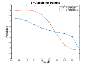
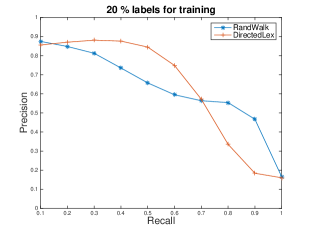
Figure 3: Recall and precision in the web spam classification experiment. Each data point shown was computed as an average over 100 runs. The largest standard deviation of the mean precision across the plotted recall values was less than 1.3 %. The algorithm of Zhou et al. (2007) appears as RandWalk. Our directed lex-minimization algorithm appears as DirectedLex.

For comparison, in Appendix C, we show the performance of our algorithm and that of Zhou et al. (2007) both with link directions reversed, as well as the performance of undirected lex-minimization and Laplacian inference, all of which are significantly worse.

7 $l_{0}$-Regularization of Vertex Values

We now explain how we can accommodate noise in both the given voltages and in the given lengths of edges. We can find the minimum number of labels to ignore, or the minimum increase in edges lengths needed so that there exists an extension whose gradients have $l_{\infty}$-norm lower than a given target. After determining which labels to ignore or the needed increment in edge lengths, we recommend computing a lex minimizer.

The algorithms we present in this section are essentially the same for directed and undirected graphs.

7.1 $l_{0}$-Vertex Regularization for Inf-minimization

The $l_{0}$-regularization of vertex labels can be viewed as a problem of outlier removal: the vector we compute is allowed to disagree with $v_{0}$ on up to $k$ terminals. Given a voltage assignment $v$ and a subset $T\subset V$ of the vertices, by $v(T)$ we mean the vector obtained by restricting $v$ to $T$. We define the $l_{0}$-Vertex Regularization for $l_{\infty}$ problem to be

$$\min_{v\in{\rm I\kern-2.0ptR}^{n}}\,\,\left\|\mathsf{grad}_{G}[v]\right\|_{\infty}\qquad\text{subject to }\left\|v(T)-v_{0}(T)\right\|_{0}\leq k,$$ (3)

where $v(T)$ is the vector of values of $v$ on the terminals $T$.

In Appendix D, we describe an approximation algorithm Approx-Outlier that approximately solves program (3). The precise statement we prove in Appendix D is given in the following theorem.

Theorem 7.1 (Approximate $l_{0}$-vertex regularization)

The algorithm Approx-Outlier takes a positive integer $k$ and a partially-labeled graph $(G,v_{0})$, and outputs an assignment $v$ with $\left\|v(T)-v_{0}(T)\right\|_{0}\leq 2k$, and $\left\|\mathsf{grad}_{G}[v]\right\|_{\infty}\leq\alpha^{*}$, where $\alpha^{*}$ is the optimum value of program (3). The algorithm runs in time $O(k(m+n\log n))$.

In Appendix D, we also describe an algorithm Outlier that exactly solves program (3) in polynomial time, and we prove its correctness.

Theorem 7.2 (Exact $l_{0}$-vertex regularization)

The algorithm Outlier takes a positive integer $k$ and a partially-labeled graph $(G,v_{0})$ solves program (3) exactly. The algorithm runs in polynomial time.

We give a proof of Theorem 7.2 in Appendix D. To do this, we reduce the program (3) to the problem of minimizing the required $l_{0}$-budget needed to achieve a fixed gradient $\alpha$ using a binary search over a set of $O(n^{2})$ gradients. This latter problem we reduce in polynomial time to Minimum Vertex Cover (VC) on a transitively closed, directed acyclic graph (a TC-DAG). VC on a TC-DAG can be solved exactly in polynomial time by a reduction to the Maximum Bipartite Matching Problem (Fulkerson (1956)). The problem was phrased by Fulkerson as one of finding a maximum antichain of a finite poset. Any transitively closed DAG corresponds directly to the comparability graph of a poset. A maximum antichain of a poset is a maximum independent set of a the comparability graph of the poset, and hence its complement is a minimum vertex cover of the comparability graph. We refer to the algorithm developed by Fulkerson as Konig-Cover.

Theorem 7.3

The algorithm Konig-Cover computes a minimum vertex cover for any transitively closed DAG $G$ in polynomial time.

7.2 Hardness of $l_{0}$ regularization for $l_{2}$

The result that $l_{0}$-regularized inf-minimization can be solved exactly in polynomial time is surprising, especially because the analogous problem for 2-Laplacian minimization turns out to be NP-Hard.

We define the the $l_{0}$ vertex regularization for $l_{2}$ for a partially-labeled graph $(G,v_{0})$ and an integer $k$ by

$$\min_{v\in\mathbb{R}^{n}\mathrel{\mathop{\mathchar 58\relax}}\left\|v(T)-v_{0}(T)\right\|_{0}\leq k}v^{T}Lv,$$

where $L$ is the Laplacian of $G$.

Theorem 7.4

$l_{0}$ vertex regularization for $l_{2}$ is NP-Hard.

In Appendix E we prove Theorem 7.4 by giving a polynomial time (Karp) reduction from the NP-Hard minimum bisection problem to $l_{0}$ vertex regularization for $l_{2}$.

8 $l_{1}$-Edge and Vertex Regularization of Inf-minimizers

Consider a partially-labeled graph $(G,v_{0})$ and an $\alpha>0$. The set of voltage assignments given by

$$\left\{v\mathrel{\mathop{\mathchar 58\relax}}v\text{ extends }v_{0}\text{ and }\left\|\mathsf{grad}_{G}[v]\right\|_{\infty}\leq\alpha\right\}$$

is convex. Going further, let us consider the edge lengths in a graph to be specified by a vector $\ell\in{\rm I\kern-2.0ptR}^{E}$. Now the set of voltages $v$ and and lengths $\ell$ which achieve $\|\mathsf{grad}_{G(\ell)}[v]\|_{\infty}\leq\alpha$ is jointly convex in $v$ and $\ell$. To see this, observe that

$$\|\mathsf{grad}_{G(\ell)}[v]\|_{\infty}\leq\alpha\Leftrightarrow\forall(u,v)\in E\mathrel{\mathop{\mathchar 58\relax}}\,{-\alpha\ell(u,v)}\leq v(u)-v(v)\leq\alpha\ell(u,v).$$ (4)

Furthermore, the condition “$v$ extends $v_{0}$” is a linear constraint on $v$, which we express as $v(T)=v_{0}(T)$. From the above, it is clear that the gradient condition corresponds to a convex set, as it is an intersection of half-spaces. These half-spaces are given by $O(m)$ linear inequalities. We can leverage this to phrase many regularized variants of inf-minimization as convex programs, and in some cases linear programs.

For example, we may consider a variant of inf-minimization combined with an $l_{1}$-budget for changing lengths of edges and values on terminals. Given a parameter $\gamma>0$ which specifies the relative cost of regularizing terminals to regularizing edges, the problem is as follows

$$\operatorname*{arg\,min}_{v\in{\rm I\kern-2.0ptR}^{n},s\in{\rm I\kern-2.0ptR}^{m},s\geq 0}\,\left\|s\right\|_{1}+\gamma\left\|v(T)-v_{0}(T)\right\|_{1}\\ \qquad\text{subject to }\left\|\mathsf{grad}_{G(\ell+s)}[v]\right\|_{\infty}\leq\alpha.$$ (5)

From our observation (4), it follows that problem (5) may be expressed as a linear program with $O(n)$ variables and $O(m)$ constraints. We can use ideas from Daitch and Spielman (2008) to solve the resulting linear program in time $\widetilde{O}(m^{1.5})$ by an interior point method with a special purpose linear equation solver. The reason is that the linear equations the IPM must solve at each iteration may be reduced to linear equations in symmetric, diagonally dominant matrices, and these may be solved in nearly-linear time (Cohen et al. (2014)).

Conclusion.

We propose the use of inf and lex minimizers for regression on graphs. We present simple algorithms for computing them that are provably fast and correct, and can also be implemented efficiently. We also present a framework and polynomial time algorithms for regularization in this setting. The initial experiments reported in the paper indicate that these algorithms give pretty good results on real and synthetic datasets. The results seem to compare quite favorably to other algorithms, particularly in the regime of tiny labeled sets. We are testing these algorithms on several other graph learning questions, and plan to report on them in a forthcoming experimental paper. We believe that inf and lex minimizers, and the associated ideas presented in the paper, should be useful primitives that can be profitably combined with other approaches to learning on graphs.

Appendix A Basic Properties of Lex-Minimizers

A.1 Meta Algorithm

Algorithm 1: Algorithm Meta-Lex: Given a well-posed instance $(G,v_{0})$, outputs $\mathsf{lex}_{G}[v_{0}]$. for $i=1,2,\ldots\mathrel{\mathop{\mathchar 58\relax}}$ 1. if $T(v_{i-1})=V_{G},$ then return $v_{i-1}$. 2. $E^{\prime}=E_{G}\setminus(T(v_{i-1})\times T(v_{i-1}))$, $G^{\prime}\mathrel{\mathop{\mathchar 58\relax}}=(V_{G},E^{\prime})$. 3. Let $P^{\star}_{i}$ be a steepest fixable path in $(G^{\prime},v_{i-1}).$ Let $\alpha^{\star}_{i}\leftarrow\nabla P^{\star}(v_{i-1}).$ 4. $v_{i}\leftarrow\mathsf{fix}[v_{i-1},P^{\star}_{i}].$

In this subsection, we prove the results that appeared in section 2. We start with a simple observation.

Proposition A.1

Given a well-posed instance $(G,v_{0})$ such that $T(v_{0})\neq V,$ let $P$ be a steepest fixable path in $(G,v_{0}).$ Then, $\mathsf{fix}[v_{0},P]$ extends $v_{0},$ and $(G,\mathsf{fix}[v_{0},P])$ is also a well-posed instance.

The properties we prove below do not depend on the choice of the steepest fixable path.

Proposition A.2

For any well-posed instance $(G,v_{0}),$ with $|V_{G}|=n,$ Meta-Lex$(G,v_{0})$ terminates in at most $n$ iterations, and outputs a complete voltage assignment $v$ that extends $v_{0}.$

• Proof of Proposition A.2:   By Proposition A.1, at any iteration $i,$ $v_{i-1}$ extends $v_{0}$ and $(G^{\prime},v_{i-1})$ is a well-posed instance. Meta-Lex only outputs $v_{i-1}$ iff $T(v_{i-1})=V,$ which means $v_{i-1}$ is a complete voltage assignment. For any $v_{i-1}$ that is not complete, for any $x\in V\setminus T(v_{i-1}),$ we must have a free terminal path in $(G^{\prime},v_{i-1})$ that contains $x$. Hence, a steepest fixable path $P^{\star}_{i}$ exists in $(G^{\prime},v_{i-1}).$ Since $P^{\star}_{i}$ is a free terminal path, $\mathsf{fix}[v_{i-1},P^{\star}_{i}]$ fixes the voltage for at least one non-terminal. Thus, Meta-Lex$(G,v_{0})$ must complete in at most $n$ iterations. $\Box$

For the following lemmas, consider a run of Meta-Lex with well-posed instance $(G,v_{0})$ as input. Let $v_{\mathsf{out}}$ be the complete voltage assignment output by Meta-Lex. Let $E_{i}$ be the set of edges $E^{\prime}$ and $G_{i}$ be the graph $G^{\prime}$ constructed in iteration $i$ of Meta-Lex.

Lemma A.3

For every edge $e\in E_{i-1}\setminus E_{i},$ we have $\left|\mathsf{grad}[v_{\mathsf{out}}](e)\right|\leq\alpha_{i}^{\star}.$ Moreover, $\alpha^{\star}_{i}$ is non-increasing with $i.$

• Proof of Lemma A.3:   Let $P^{\star}_{i}=(x_{0},\ldots,x_{r})$ be a steepest fixable path in iteration $i$ (when we deal with instance $(G_{i-1},v_{i-1})$). Consider a terminal path $P_{i+1}$ in $(G_{i},v_{i})$ such that $\{\partial_{0}P_{i+1},\partial_{1}P_{i+1}\}\cap(T(v_{i})\setminus T(v_{i-1}))\neq\emptyset.$ We claim that $\nabla P_{i+1}(v_{i})\leq\alpha^{\star}_{i}.$ On the contrary, assume that $\nabla P_{i+1}(v_{i})>\alpha^{\star}_{i}.$ Consider the case $\partial_{0}P_{i+1}\in T(v_{i})\setminus T(v_{i-1}),\partial_{1}P_{1}\in T(v_{i-1}).$ By the definition of $v_{i},$ we must have $\partial_{0}P_{i+1}=x_{j}$ for some $j\in[r-1].$ Let $P^{\prime}_{i+1}$ be the path formed by joining paths $P^{\star}_{i}[x_{0}\mathrel{\mathop{\mathchar 58\relax}}x_{j}]$ and $P_{i+1}.$ $P^{\prime}_{i+1}$ is a free terminal path in $(G_{i-1},v_{i-1}).$ We have,

  $$v_{i-1}(x_{0})-v_{i-1}(\partial_{1}P_{i+1}) =(v_{i}(x_{0})-v_{i}(x_{j}))+(v_{i}(\partial_{0}P_{i+1})-v_{i}(\partial_{1}P_{i+1}))$$

  $$>\alpha^{\star}_{i}\cdot\ell(P_{i}^{\star}[x_{0}\mathrel{\mathop{\mathchar 58\relax}}x_{j}])+\alpha^{\star}_{i}\cdot\ell(P_{i+1})=\alpha^{\star}_{i}\cdot\ell(P_{i+1}^{\prime}),$$

  giving $\nabla P^{\prime}_{i+1}(v_{i})>\alpha^{\star}_{i},$ which is a contradiction since the steepest fixable path $P^{\star}_{i}$ in $(G_{i-1},v_{i-1})$ has gradient $\alpha^{\star}_{i}$. The other cases can be handled similarly.

  Applying the above claim to an edge $e\in E_{i-1}\setminus E_{i},$ whose gradient is fixed for the first time in iteration $i,$ we obtain that $\mathsf{grad}[v_{i+1}](e)\leq\alpha_{i}^{\star}.$ If $v$ is the complete voltage assignment output by Meta-Lex, since $v$ extends $v_{i+1},$ we get $\mathsf{grad}[v_{\mathsf{out}}](e)\leq\alpha^{\star}_{i}$. Applying the claim to the symmetric edge, we obtain $-\mathsf{grad}[v_{\mathsf{out}}](e)\leq\alpha_{i}^{\star},$ implying $|\mathsf{grad}[v_{\mathsf{out}}](e)|\leq\alpha_{i}^{\star}.$

Consider any free terminal path $P_{i+1}$ in $(G_{i},v_{i}).$ If $P_{i+1}$ is also a terminal path in $(G_{i-1},v_{i-1}),$ it is a free terminal path in $(G_{i-1},v_{i-1}).$ In addition, since a steepest fixable path $P^{\star}_{i}$ in $(G_{i-1},v_{i-1})$ has $\nabla P^{\star}_{i}=\alpha^{\star}_{i},$ we get $\nabla P_{i+1}(v_{i})=\nabla P_{i+1}(v_{i-1})\leq\alpha_{i}^{\star}.$ Otherwise, we must have $\{\partial_{0}P_{i+1},\partial_{1}P_{i+1}\}\cap(T(v_{i})\setminus T(v_{i-1}))\neq\emptyset,$ and we can deduce $\nabla P_{i+1}(v_{i})\leq\alpha_{i}^{\star}$ using the above claim. Thus, all free terminal paths $P_{i+1}$ in $(G_{i},v_{i})$ satisfy $\nabla P_{i+1}(v_{i})\leq\alpha^{\star}_{i}.$ In particular, $\alpha^{\star}_{i+1}=\nabla P^{\star}_{i+1}(v_{i})\leq\alpha^{\star}_{i}.$ Thus, $\alpha^{\star}_{i}$ is non-increasing with $i.$ $\Box$

Lemma A.4

For any complete voltage assignment $v$ for $G$ that extends $v_{0},$ if $v\neq v_{\mathsf{out}},$ we have $\mathsf{grad}[v]\not\preceq\mathsf{grad}[v_{\mathsf{out}}],$ and hence $\mathsf{grad}[v_{\mathsf{out}}]\preceq\mathsf{grad}[v].$

• Proof of Lemma A.4:   Consider any complete voltage assignment $v$ for $G$ that extends $v_{0},$ such that $v\neq v_{\mathsf{out}}.$ Thus, there exists a unique $i$ such that $v$ extends $v_{i-1}$ but does not extend $v_{i}.$ We will argue that $\mathsf{grad}[v]\not\preceq\mathsf{grad}[v_{\mathsf{out}}],$ and hence $\mathsf{grad}[v_{\mathsf{out}}]\preceq\mathsf{grad}[v].$ For every edge $e\in E\setminus E_{i-1}$ that has been fixed so far, $\mathsf{grad}[v](e)=\mathsf{grad}[v_{i-1}](e)=\mathsf{grad}[v_{\mathsf{out}}](e),$ and hence we can ignore these edges.

  Since $v$ extends $v_{i-1}$ but not $v_{i},$ there exists an $x\in T(v_{i})\setminus T(v_{i-1})$ such that $v(x)\neq v_{i}(x)=v_{\mathsf{out}}(x).$ Assume $v(x)<v_{i}(x)$ (the other case is symmetric). If $P^{\star}_{i}=(x_{0},\ldots,x_{r})$ is the steepest fixable path with gradient $\alpha^{\star}_{i}$ picked in iteration $i,$ we must have $x=x_{j}$ for some $j\in[r-1].$ Thus,

  $$\sum_{k=1}^{j}(v(x_{k-1})-v(x_{k}))=v(x_{0})-v(x_{j})>v_{i}(x_{0})-v_{i}(x_{j})=\alpha^{\star}_{i}\cdot\ell(P^{\star}_{i}[x_{0}\mathrel{\mathop{\mathchar 58\relax}}x_{j}])=\alpha^{\star}_{i}\cdot\sum_{k=1}^{j}\ell(x_{k-1},x_{k}).$$

  Thus, for some $k\in[j],$ we must have $\mathsf{grad}[v](x_{k-1},x_{k})>\alpha_{i}^{\star}.$ Since $P^{*}_{i}$ is a path in $G_{i-1}$, we have $\{x_{k-1},x_{k}\}\not\subseteq T(v_{i-1})$. This gives $(x_{k-1},x_{k})\in(E_{i-1}\setminus E_{i}).$ But then, from Lemma A.3, it follows that for all $e\in(E_{i-1}\setminus E_{i}),$ we have $|\mathsf{grad}[v_{\mathsf{out}}](e)|\leq\alpha_{i}^{\star}.$ Thus, we have $\mathsf{grad}[v]\not\preceq\mathsf{grad}[v_{\mathsf{out}}].$ $\Box$

Lemma A.5

Let $P=(x_{0},\ldots,x_{r})$ be a steepest fixable path such that it does not have any edges in $T(v_{0})\times T(v_{0})$ and $v_{1}=\mathsf{fix}_{G}[v_{0},P]$. Then for every $i\in[r],$ we have $\mathsf{grad}[v_{1}](x_{i-1},x_{i})=\nabla P.$

• Proof of Lemma A.5:   Suppose this is not true and let $j\in[r]$ be the minimum number such that $\mathsf{grad}[v_{1}](x_{j-1},x_{j})\neq\nabla P.$ By definition of $v_{1}$ we would necessarily have $j<r$ and $v_{j}\in T(v_{0}).$ Suppose $\mathsf{grad}[v_{1}](x_{j-1},x_{j})<\nabla P.$ We would then have $v_{1}(x_{0})-v_{1}(x_{j})<\nabla P*\ell(P[x_{0}\mathrel{\mathop{\mathchar 58\relax}}x_{j}]).$ Since $P$ does not have any edges in $T(v_{0})\times T(v_{0})$, $P_{1}\mathrel{\mathop{\mathchar 58\relax}}=(x_{j},...,x_{r})$ would be a free terminal path with $\nabla P_{1}>\nabla P.$ This is a contradiction. Other cases can be ruled out similarly.

  $\Box$

• Proof of Theorem 3.3:   Consider an arbitrary run of Meta-Lex on $(G,v_{0}).$ Let $v_{\mathsf{out}}$ be the complete voltage assignment output by Meta-Lex. Proposition A.1 implies that $v_{\mathsf{out}}$ extends $v_{0}.$ Lemma A.4 implies that for any complete voltage assignment $v\neq v_{\mathsf{out}}$ that extends $v_{0},$ we have $\mathsf{grad}[v_{\mathsf{out}}]\preceq\mathsf{grad}[v].$ Thus, $v_{\mathsf{out}}$ is a lex-minimizer. Moreover, the lemma also gives that for any such $v,$ $\mathsf{grad}[v]\not\preceq\mathsf{grad}[v_{\mathsf{out}}].$ and hence $v_{\mathsf{out}}$ is a unique lex-minimizer. Thus, $v_{\mathsf{out}}$ is the unique voltage assignment satisfying Def. 2.1, and we denote it as $\mathsf{lex}_{G}[v_{0}].$ Since we started with an arbitrary run of Meta-Lex, uniqueness implies that every run of Meta-Lex on $(G,v_{0})$ must output $\mathsf{lex}_{G}[v_{0}].$ $\Box$

• Proof of Lemma 3.5:   Suppose we have a complete voltage assignment $v$ extending $v_{0},$ such that $\left\|\mathsf{grad}[v]\right\|_{\infty}\leq\alpha.$ For any terminal path $P=(x_{0},\ldots,x_{r}),$ we get,

  $$\nabla P(v_{0})=v_{0}(\partial_{0}P)-v_{0}(\partial_{1}P)=v(\partial_{0}P)-v(\partial_{1}P)=\sum_{i=1}^{r}\mathsf{grad}[v](x_{i-1},x_{i})\leq\alpha\cdot\sum_{i=1}^{r}\ell(x_{i-1},x_{i})=\alpha\cdot\ell(P),$$

  giving $\nabla P(v_{0})\leq\alpha.$

  On the other hand, suppose every terminal path $P$ in $(G,v_{0})$ satisfies $\nabla P(v_{0})\leq\alpha.$ Consider $v=\mathsf{lex}_{G}[v_{0}].$ We know that $v$ extends $v_{0}.$ For every edge $e\in E_{G}\cap T(v_{0})\times T(v_{0}),$ $e$ is a (trivial) terminal path in $(G,v_{0}),$ and hence has satisfies $\mathsf{grad}[v](e)=\mathsf{grad}[v_{0}](e)=\nabla{e}(v_{0})\leq\alpha.$ Considering the reverse edge, we also obtain $-\mathsf{grad}[v](e)\leq\alpha.$ Thus, $|\mathsf{grad}[v](e)|\leq\alpha.$ Moreover, using Lemma A.3, we know that for edge $e\in E_{G}\setminus T(v_{0})\times T(v_{0}),$ $|\mathsf{grad}[v](e)|\leq\alpha_{1}^{\star}=\nabla P_{1}^{\star}\leq\alpha$ since $P_{1}$ is a terminal path in $(G,v_{0}).$ Thus, for every $e\in E_{G},$ $|\mathsf{grad}[v](e)|\leq\alpha,$ and hence $\left\|\mathsf{grad}[v]\right\|_{\infty}\leq\alpha.$ $\Box$

A.2 Stability

In this subsection, we sketch a proof of the monotonicity of lex-minimizers and show how it implies the stability property claimed earlier.

For any well-posed $(G,v_{0}),$ there could be several possible executions of Meta-Lex, each characterized by the sequence of paths $P^{\star}_{i}.$ We can apply Theorem 3.3 to deduce the following structural result about the lex-minimizer.

Corollary A.6

For any well-posed instance $(G,v_{0}),$ consider a sequence of paths $(P_{1},\ldots,P_{r})$ and voltage assignments $(v_{1},\ldots,v_{r})$ for some positive integer $r$ such that:

1. $P^{\star}_{i}$ is a steepest fixable path in $(G_{i-1},v_{i-1})$ for $i=1,\ldots,r.$

2. $v_{i}=\mathsf{fix}[v_{i-1},P^{\star}_{i}]$ for $i=1,\ldots,r.$

3. $T(v_{r})=V_{G}.$

Then, we have $v_{r}=\mathsf{lex}_{G}[v_{0}].$

We call such a sequence of paths and voltages to be a decomposition of $\mathsf{lex}_{G}[v_{0}].$ Again, note that $\mathsf{lex}_{G}[v_{0}]$ can possibly have multiple decompositions. However, any two such decompositions are consistent in the sense that they produce the same voltage assignment.

• Proof of Corollary 3.7:   We first define some operations on partial assignments which simplifies the notation. Let $v_{0},v_{1}$ be any two partial assignments with the same set of terminals $T\mathrel{\mathop{\mathchar 58\relax}}=T(v_{0})=T(v_{1})$ and $c,d\in\mathbb{R}$. By $cv_{0}+d$ we mean a partial assignment $v$ with $T(v)=T$ satisfying $v(t)=cv_{0}(t)+d$ for all $t\in T$. Also, by $v_{0}+v_{1}$ we mean a partial assignment $v$ with $T(v)=T$ satisfying $v(t)=v_{0}(t)+v_{1}(t)$ for all $t\in T.$ Also, we say $v_{1}\geq v_{0}$ if $v_{1}(t)\geq v_{0}(t)$ for all $t\in T$.

Now we can show how Corollary 3.7 follows from Theorem 3.6. Let $v\mathrel{\mathop{\mathchar 58\relax}}=v_{1}-v_{0}$, and $\left\|v\right\|_{\infty}=\epsilon$, for some $\epsilon>0.$ Therefore, $v_{0}+\epsilon\geq v_{1}\geq v_{0}-\epsilon.$ Theorem 3.6 then implies that $\mathsf{lex}_{G}[v_{0}]+\epsilon\geq\mathsf{lex}[v_{1}]\geq\mathsf{lex}[v_{0}]-\epsilon,$ hence proving the corollary. $\Box$

• Proof sketch of Theorem 3.6:   It is easy to see that the first statement holds. For the second statement, we first observe that if there is a sequence of paths $P_{1},...,P_{r}$ that is simultaneously a decomposition of both $\mathsf{lex}[v_{0}]$ and $\mathsf{lex}[v_{1}]$, then this is easy to see. If such a path sequence doesn’t exist, then we look at $v_{t}\mathrel{\mathop{\mathchar 58\relax}}=v_{0}+t(v_{1}-v_{0})$. We state here without a proof (though the proof is elementary) that we can then split the interval $[0,1]$ into finitely many subintervals $[a_{0},a_{1}],[a_{1},a_{2}],..,[a_{k-1},a_{k}]$, with $a_{0}=0,a_{k}=1$, such that for any $i$, there is a path sequence $P_{1},...,P_{r}$ which is a decomposition of $\mathsf{lex}[v_{t}]$ for all $t\in[a_{i},a_{i+1}]$. We then observe that $v_{0}=v_{a_{0}}\leq v_{a_{1}}\leq...v_{a_{k}}=v_{1}.$ Since for every $a_{i},a_{i+1}$, there is a path sequence which is simultaneously a decomposition of both $\mathsf{lex}[v_{a_{i}}]$ and $\mathsf{lex}[v_{a_{i+1}}]$, we immediately get

  $$\mathsf{lex}[v_{0}]=\mathsf{lex}[v_{a_{0}}]\leq\mathsf{lex}[v_{a_{1}}]\leq...\leq\mathsf{lex}[v_{a_{k}}]=\mathsf{lex}[v_{1}].$$

  $\Box$

A.3 Alternate Characterizations

• Proof of Theorem 3.10:   We know that $\mathsf{lex}_{G}[v_{0}]$ extends $v_{0}.$ We first prove that $v=\mathsf{lex}_{G}[v_{0}]$ satisfies the max-min gradient averaging property. Assume to the contrary. Thus, there exists $x\in V_{G}\setminus T(v_{0})$ such that

  $$\max_{y\mathrel{\mathop{\mathchar 58\relax}}(x,y)\in E_{G}}\mathsf{grad}[v](x,y)\neq-\min_{y\mathrel{\mathop{\mathchar 58\relax}}(x,y)\in E_{G}}\mathsf{grad}[v](x,y).$$

  Assume that $\max_{(x,y)\in E_{G}}\mathsf{grad}[v](x,y)\geq-\min_{(x,y)\in E_{G}}\mathsf{grad}[v](x,y).$ Then, consider $v^{\prime}$ extending $v_{0}$ that is identical to $v$ except for $v^{\prime}(x)=v(x)-\epsilon$ for $\epsilon>0.$ For $\epsilon$ small enough, we get that

  $$\max_{y\mathrel{\mathop{\mathchar 58\relax}}(x,y)\in E_{G}}\mathsf{grad}[v^{\prime}](x,y)<\max_{y\mathrel{\mathop{\mathchar 58\relax}}(x,y)\in E_{G}}\mathsf{grad}[v](x,y)$$

  and

  $$-\min_{y\mathrel{\mathop{\mathchar 58\relax}}(x,y)\in E_{G}}\mathsf{grad}[v^{\prime}](x,y)<\max_{y\mathrel{\mathop{\mathchar 58\relax}}(x,y)\in E_{G}}\mathsf{grad}[v](x,y).$$

  The gradient of edges not incident on the vertex $x$ is left unchanged. This implies that $\mathsf{grad}[v]\not\preceq\mathsf{grad}[v^{\prime}],$ contradicting the assumption that $v$ is the lex-minimizer. (The other case is similar).

  For the other direction. Consider a complete voltage assignment $v$ extending $v_{0}$ that satisfies the max-min gradient averaging property w.r.t. $(G,v_{0}).$ Let

  $$\alpha=\max_{\begin{subarray}{c}(x,y)\in E_{G}\\ x\in V\setminus T(v_{0})\end{subarray}}\mathsf{grad}[v](x,y)\geq 0$$

  be the maximum edge gradient, and consider any edge $(x_{0},x_{1})\in E_{G}$ such that $\mathsf{grad}[v](x_{1},x_{0})=\alpha,$ with $x_{1}\in V\setminus T(v_{0}).$ If $\alpha=0,$ $\mathsf{grad}[v]$ is identically zero, and is trivially the lex-minimal gradient assignment. Thus, both $v$ and $\mathsf{lex}_{G}[v_{0}]$ are constant on each connected component. Since $(G,v_{0})$ is well-posed, there is at least one terminal in each component, and hence $v$ and $\mathsf{lex}_{G}[v_{0}]$ must be identical.

  Now assume $\alpha>0.$ By the max-min gradient averaging property, $\exists x_{2}\in V_{G}$ such that $(x_{1},x_{2})\in E_{G}$ and

  $$\mathsf{grad}[v](x_{1},x_{2})=\min_{y\mathrel{\mathop{\mathchar 58\relax}}(x_{1},y)\in E_{G}}\mathsf{grad}[v](x_{1},y) =-\max_{y\mathrel{\mathop{\mathchar 58\relax}}(x_{1},y)\in E_{G}}\mathsf{grad}[v](x_{1},y)$$

  $$\leq-\mathsf{grad}[v](x_{1},x_{0})=-\alpha.$$

  Thus, $\mathsf{grad}[v](x_{2},x_{1})\geq\alpha.$ Since $\alpha$ is the maximum edge gradient, we must have $\mathsf{grad}[v](x_{2},x_{1})=\alpha.$ Moreover, $v(x_{2})>v(x_{1})>v(x_{0}),$ thus $x_{2}\neq x_{0}.$ We can inductively apply this argument at $x_{2}$ until we hit a terminal. Similarly, if $x_{0}\notin T(v_{0})$ we can extend the path in the other direction. Consequently, we obtain a path $P=(x_{j},\ldots,x_{2},x_{1},x_{0},x_{-1},\ldots,x_{k})$ with all vertices as distinct, such that $x_{j},x_{k}\in T(v_{0}),$ and $x_{i}\in V\setminus T(v_{0})$ for all $i\in[j+1,k-1].$ Moreover, $\mathsf{grad}[v](x_{i},x_{i-1})=\alpha$ for all $j<i\leq k.$ Thus, $P$ is a free terminal path with $\nabla P[v_{0}]=\alpha.$

  Moreover, since $v$ is a voltage assignment extending $v_{0}$ with $\left\|\mathsf{grad}[v]\right\|_{\infty}=\alpha,$ using Lemma 3.5, we know that every terminal path $P^{\prime}$ in $(G,v_{0})$ must satisfy $\nabla P^{\prime}(v_{0})\leq\alpha.$ Thus, $P$ is a steepest fixable path in $(G,v_{0}).$ Thus, letting $v_{1}=\mathsf{fix}[v_{0},P],$ using Corollary 3.4, we obtain that $\mathsf{lex}_{G}[v_{1}]=\mathsf{lex}_{G}[v_{0}].$ Moreover, since $\alpha=\nabla P[v_{0}]=\mathsf{grad}[v](x_{i},x_{i-1})$ for all $i\in(j,k],$ we get $v_{1}(x_{i})=v(x_{i})$ for all $i\in(j,k).$ Thus, $v$ extends $v_{1}.$

  We can iterate this argument for $r$ iterations until $T(v_{r})=V_{G},$ giving $v=v_{r}$ and $v_{r}=\mathsf{lex}_{G}[v_{r}]=\mathsf{lex}_{G}[v_{0}].$ (Since we are fixing at least one terminal at each iteration, this procedure terminates). Thus, we get $v=\mathsf{lex}_{G}[v_{0}].$ $\Box$

Appendix B Description of the Algorithms

Algorithm 2: ModDijkstra$(G,v_{0},\alpha)$: Given a well-posed instance $(G,v_{0}),$ a gradient value $\alpha\geq 0,$ outputs a complete voltage assignment $v$ for $G,$ and an array $\mathsf{parent}\mathrel{\mathop{\mathchar 58\relax}}V\to V\cup\{\mathsf{null}\}.$ 1. for $x\in V_{G},$ 2. Add $x$ to a fibonacci heap, with ${\mathsf{key}}(x)=+\infty.$ 3. $\mathsf{finished}(x)\leftarrow\mbox{\bf false\ }$ 4. for $x\in T(v_{0})$ 5. Decrease ${\mathsf{key}}(x)$ to $v_{0}(x).$ 6. $\mathsf{parent}(x)\leftarrow\mathsf{null}.$ 7. while heap is not empty 8. $x\leftarrow$ pop element with minimum $\mathsf{key}$ from heap 9. $v(x)\leftarrow{\mathsf{key}}(x).$ ${\mathsf{finished}}(x)\leftarrow\mbox{\bf true\ }.$ 10. for $y\mathrel{\mathop{\mathchar 58\relax}}(x,y)\in E_{G}$ 11. if ${\mathsf{finished}}(y)=\mbox{\bf false\ }$ 12. if ${\mathsf{key}}(y)>v(x)+\alpha\cdot\ell(x,y)$ 13. Decrease ${\mathsf{key}}(y)$ to $v(x)+\alpha\cdot\ell(x,y).$ 14. $\mathsf{parent}(y)\leftarrow x.$ 15. return $(v,\mathsf{parent})$

Theorem B.1

For a well-posed instance $(G,V_{0})$ and a gradient value $\alpha\geq 0,$ let $(v,\mathsf{parent})\leftarrow$ ModDijkstra$(G,v_{0},\alpha).$ Then, $v$ is a complete voltage assignment such that, $\forall x\in V_{G},$ $v(x)=\min_{t\in T(v_{0})}\{v_{0}(t)+\alpha{\mathsf{dist}}(x,t)\}.$ Moreover, the pointer array $\mathsf{parent}$ satisfies $\forall x\notin T(v_{0}),$ $\mathsf{parent}(x)\neq{\mathsf{null}}$ and $v(x)=v(\mathsf{parent}(x))+\alpha\cdot\ell(x,\mathsf{parent}(x)).$

Algorithm 3: Algorithm CompVLow$(G,v_{0},\alpha)$: Given a well-posed instance $(G,v_{0}),$ a gradient value $\alpha\geq 0,$ outputs $\mathsf{vLow},$ a complete voltage assignment for $G,$ and an array $\mathsf{LParent}$ $\mathrel{\mathop{\mathchar 58\relax}}V\to V\cup\{\mathsf{null}\}$. 1. $(\mathsf{vLow},\mathsf{LParent})\leftarrow$ ModDijkstra$(G,v_{0},\alpha)$ 2. return $(\mathsf{vLow},\mathsf{LParent})$

Algorithm 4: Algorithm CompVHigh$(G,v_{0},\alpha)$: Given a well-posed instance $(G,v_{0}),$ a gradient value $\alpha\geq 0$, outputs $\mathsf{vHigh},$ a complete voltage assignment for $G$, and an array $\mathsf{HParent}\mathrel{\mathop{\mathchar 58\relax}}V\to V\cup\{\mathsf{null}\}$. 1. for $x\in V_{G}$ 2. if $x\in T(v_{0})$ then $v_{1}(x)\leftarrow-v_{0}(x)$ else $v_{1}(x)\leftarrow v_{1}(x).$ 3. $(\mathsf{temp},\mathsf{HParent})\leftarrow$ ModDijkstra$(G,v_{1},\alpha)$ 4. for $x\in V_{G}\mathrel{\mathop{\mathchar 58\relax}}\mathsf{vHigh}(x)\leftarrow-\mathsf{temp}(x)$ 5. return $(\mathsf{vHigh},\mathsf{HParent})$

Corollary B.2

For a well-posed instance $(G,V_{0})$ and a gradient value $\alpha\geq 0,$ let $(\mathsf{vLow}[\alpha],\mathsf{LParent})\leftarrow$ CompVLow$(G,v_{0},\alpha)$ and $(\mathsf{vHigh}[\alpha],\mathsf{HParent})\leftarrow$ CompVHigh$(G,v_{0},\alpha).$ Then, $\mathsf{vLow}[\alpha],\mathsf{vHigh}[\alpha]$ are complete voltage assignments for $G$ such that, $\forall x\in V_{G},$

$$\mathsf{vLow}[\alpha](x)=\min_{t\in T(v_{0})}\{v_{0}(t)+\alpha\cdot{\mathsf{dist}}(x,t)\} \mathsf{vHigh}[\alpha](x)=\max_{t\in T(v_{0})}\{v_{0}(t)-\alpha\cdot{\mathsf{dist}}(t,x)\}.$$

Moreover, the pointer arrays $\mathsf{LParent},\mathsf{HParent}$ satisfy $\forall x\notin T(v_{0}),$ $\mathsf{LParent}(x),\mathsf{HParent}(x)\neq{\mathsf{null}}$ and

$$\mathsf{vLow}[\alpha](x) =\mathsf{vLow}[\alpha](\mathsf{LParent}(x))+\alpha\cdot\ell(x,\mathsf{LParent}(x)),$$

$$\mathsf{vHigh}[\alpha](x) =\mathsf{vHigh}[\alpha](\mathsf{HParent}(x))-\alpha\cdot\ell(x,\mathsf{HParent}(x)).$$

Algorithm 5: Algorithm CompInfMin$(G,v_{0})$: Given a well-posed instance $(G,v_{0})$, outputs a complete voltage assignment $\mathsf{{v}}$ for $G,$ extending $v_{0}$ that minimizes $\left\|\mathsf{grad}[\mathsf{{v}}]\right\|_{\infty}$. 1. $\alpha\leftarrow\max\{|\mathsf{grad}[v_{0}](e)|\ |\ e\in E_{G}\cap(T(v_{0})\times T(v_{0}))\}.$ 2. $E_{G}\leftarrow E_{G}\setminus(T(v_{0})\times T(v_{0}))$ 3. $P\leftarrow$SteepestPath$(G,v_{0}).$ 4. $\alpha\leftarrow\max\{\alpha,\nabla P(v_{0})\}$ 5. $(\mathsf{vLow},\mathsf{LParent})\leftarrow$ CompVLow$(G,v_{0},\alpha)$ 6. $(\mathsf{vHigh},\mathsf{HParent})\leftarrow$ CompVHigh$(G,v_{0},\alpha)$ 7. for $x\in V_{G}$ 8. if $x\in T(v_{0})$ 9. then $\mathsf{v}(x)\leftarrow v_{0}(x)$ 10. else $\mathsf{{v}}(x)\leftarrow\frac{1}{2}\cdot(\mathsf{vLow}(x)+\mathsf{vHigh}(x)).$ 11. return $\mathsf{{v}}$

Algorithm 6: Algorithm CompHighPressGraph$(G,v_{0},\alpha)$: Given a well-posed instance $(G,v_{0}),$ a gradient value $\alpha\geq 0$, outputs a minimal induced subgraph $G^{\prime}$ of $G$ where every vertex has $\mathsf{pressure}[v_{0}](\cdot)>\alpha.$ 1. $(\mathsf{vLow},\mathsf{LParent})\leftarrow$ CompVLow$(G,v_{0},\alpha)$ 2. $(\mathsf{vHigh},\mathsf{HParent})\leftarrow$ CompVHigh$(G,v_{0},\alpha)$ 3. $V_{G^{\prime}}\leftarrow\{x\in V_{G}\ |\ \mathsf{vHigh}(x)>\mathsf{vLow}(x)\ \}$ 4. $E_{G^{\prime}}\leftarrow\{(x,y)\in E_{G}\ |\ x,y\in V_{G^{\prime}}\}.$ 5. $G^{\prime}\leftarrow(V^{\prime},E^{\prime},\ell)$ 6. return $G^{\prime}$

• Proof of Lemma 4.3:  

  $$\mathsf{vHigh}[\alpha](x)>\mathsf{vLow}[\alpha](x)$$

  is equivalent to

  $$\max_{t\in T(v_{0})}\{v_{0}(t)-\alpha\cdot{\mathsf{dist}}(t,x)\}>\min_{t\in T(v_{0})}\{v_{0}(t)+\alpha\cdot{\mathsf{dist}}(x,t)\},$$

  which implies that there exists terminals $s,t\in T(v_{0})$ such that

  $$v_{0}(t)-\alpha\cdot{\mathsf{dist}}(t,x)>v_{0}(s)+\alpha\cdot{\mathsf{dist}}(x,s)$$

  thus,

  $$\mathsf{pressure}[v_{0}](x)\geq\frac{v_{0}(t)-v_{0}(s)}{{\mathsf{dist}}(t,x)+{\mathsf{dist}}(x,s)}>\alpha.$$

  So the inequality on $\mathsf{vHigh}$  and $\mathsf{vLow}$  implies that pressure is strictly greater than $\alpha$. On the other hand, if $\mathsf{pressure}[v_{0}](x)>\alpha$, there exists terminals $s,t\in T(v_{0})$ such that

  $$\frac{v_{0}(t)-v_{0}(s)}{{\mathsf{dist}}(t,x)+{\mathsf{dist}}(x,s)}=\mathsf{pressure}[v_{0}](x)>\alpha.$$

  Hence,

  $$v_{0}(t)-\alpha\cdot{\mathsf{dist}}(t,x)>v_{0}(s)+\alpha\cdot{\mathsf{dist}}(x,s)$$

  which implies $\mathsf{vHigh}[\alpha](x)>\mathsf{vLow}[\alpha](x)$. $\Box$

Algorithm 7: Algorithm SteepestPath$(G,v_{0})$: Given a well-posed instance $(G,v_{0}),$ with $T(v_{0})\neq V_{G},$ outputs a steepest free terminal path $P$ in $(G,v_{0}).$ 1. Sample uniformly random $e\in E_{G}.$ Let $e=(x_{1},x_{2}).$ 2. Sample uniformly random $x_{3}\in V_{G}.$ 3. for $i=1$ to $3$ 4. $P\leftarrow$ VertexSteepestPath$(G,v_{0},x_{i})$ 5. Let $j\in\operatorname*{arg\,max}_{j\in\{1,2,3\}}\nabla P_{j}(v_{0})$ 6. $G^{\prime}\leftarrow$ CompHighPressGraph$(G,v_{0},\nabla P_{j}(v_{0}))$ 7. if $E_{G^{\prime}}=\emptyset,$ 8. then return $P_{j}$ 9. else return SteepestPath$(G^{\prime},v_{0}|_{V_{G^{\prime}}})$

Algorithm 8: Algorithm CompLexMin$(G,v_{0})$: Given a well-posed instance $(G,v_{0}),$ with $T(v_{0})\neq V_{G}$, outputs $\mathsf{lex}_{G}[v_{0}]$. 1. while $T(v_{0})\neq V_{G}$ 2. $E_{G}\leftarrow E_{G}\setminus(T(v_{0})\times T(v_{0}))$ 3. $P\leftarrow$ SteepestPath$(G,v_{0})$ 4. $v_{0}\leftarrow$ $\mathsf{fix}$$[v_{0},P]$ 5. return $v_{0}$

Algorithm 9: Algorithm VertexSteepestPath$(G,v_{0},x)$: Given a well-posed instance $(G,v_{0}),$ and a vertex $x\in V_{G}$, outputs a steepest terminal path in $(G,v_{0})$ through $x$. 1. Using Dijkstra’s algorithm, compute ${\mathsf{dist}}(x,t)$ for all $t\in T(v_{0})$ 2. if $x\in T(v_{0})$ 3. $y\leftarrow\operatorname*{arg\,max}_{y\in T(v_{0})}\frac{|v_{0}(x)-v_{0}(y)|}{{\mathsf{dist}}(x,y)}$ 4. if $v_{0}(x)\geq v_{0}(y)$ 5. then return a shortest path from $x$ to $y$ 6. else return a shortest path from $y$ to $x$ 7. else 8. for $t\notin T(v_{0}),$ $\mathsf{d}(t)\leftarrow{\mathsf{dist}}(x,t)$ 9. $(t_{1},t_{2})\leftarrow$ StarSteepestPath$(T(v_{0}),v_{0}|_{T(v_{0})},\mathsf{d})$ 10. Let $P_{1}$ be a shortest path from $t_{1}$ to $x.$ Let $P_{2}$ be a shortest path from $x$ to $t_{2}.$ 11. $P\leftarrow(P_{1},P_{2}).$ return $P.$

Algorithm 10: StarSteepestPath$(T,v,\mathsf{d})$: Returns the steepest path in a star graph, with a single non-terminal connected to terminals in $T,$ with lengths given by $\mathsf{d}$, and voltages given by $v.$ 1. Sample $t_{1}$ uniformly and randomly from $T$ 2. Compute $t_{2}\in\operatorname*{arg\,max}_{t\in T}\frac{|v(t_{1})-v(t)|}{\mathsf{d}(t_{1})+\mathsf{d}(t)}$ 3. $\alpha\leftarrow\frac{|v(t_{2})-v(t_{1})|}{\mathsf{d}(t_{1})+\mathsf{d}(t_{2})}$ 4. Compute $v_{\mathsf{low}}\leftarrow\min_{t\in T}(v(t)+\alpha\cdot{\mathsf{d}}(t))$ 5. $T_{\mathsf{low}}\leftarrow\{t\in T\ |\ v(t)>v_{\mathsf{low}}+\alpha\cdot\mathsf{{d}}(t)\}$ 6. Compute $v_{\mathsf{high}}\leftarrow\max_{t\in T}(v(t)-\alpha\cdot{\mathsf{d}}(t))$ 7. $T_{\mathsf{high}}\leftarrow\{t\in T\ |\ v(t)<v_{\mathsf{high}}-\alpha\cdot\mathsf{{d}}(t)\}$ 8. $T^{\prime}\leftarrow T_{\mathsf{low}}\cup T_{\mathsf{high}}.$ 9. if $T^{\prime}=\emptyset$ 10. then if $v(t_{1})\geq v(t_{2})$ then return $(t_{1},t_{2})$ else return $(t_{2},t_{1})$ 11. else return StarSteepestPath$(T^{\prime},v|_{T^{\prime}},\mathsf{{d}}_{T^{\prime}})$

B.1 Faster Lex-minimization

Algorithm 11: Algorithm CompFastLexMin$(G,v_{0})$: Given a well-posed instance $(G,v_{0}),$ with $T(v_{0})\neq V_{G}$, outputs $\mathsf{lex}_{G}[v_{0}]$. 1. while $T(v_{0})\neq V_{G}$ 2. $v_{0}\leftarrow$ FixPathsAbovePress$(G,v_{0},0)$ 3. return $v_{0}$

Algorithm 12: Algorithm FixPathsAbovePress$(G,v_{0},\alpha)$: Given a well-posed instance $(G,v_{0}),$ with $T(v_{0})\neq V_{G}$, and a gradient value $\alpha,$ iteratively fixes all paths with gradient $>\alpha$. 1. while $T(v_{0})\neq V_{G}$ 2. $E_{G}\leftarrow E_{G}\setminus(T(v_{0})\times T(v_{0}))$ 3. Sample uniformly random $e\in E_{G}.$ Let $e=(x_{1},x_{2}).$ 4. Sample uniformly random $x_{3}\in V_{G}.$ 5. for $i=1$ to $3$ 6. $P_{i}\leftarrow$ VertexSteepestPath$(G,v_{0},x_{i})$ 7. Let $j\in\operatorname*{arg\,max}_{j\in\{1,2,3\}}\nabla P_{j}(v_{0})$ 8. $G^{\prime}\leftarrow$ CompHighPressGraph$(G,v_{0},\nabla P_{j}(v_{0}))$ 9. if $E_{G^{\prime}}=\emptyset,$ 10. then $v_{0}\leftarrow$ $\mathsf{fix}$$[v_{0},P]$ 11. else Let $G^{\prime}_{i},i=1,\ldots,r$ be the connected components of $G^{\prime}.$ 12. for $i=1,\ldots,r$ 13. $v_{i}\leftarrow$ FixPathsAbovePress$(G^{\prime}_{i},v_{0}|_{V_{G^{\prime}_{i}}},\nabla P_{j}(v_{0}))$ 14. for $x\in V_{G^{\prime}_{i}},$ set $v_{0}(x)\leftarrow v_{i}(x)$ 15. if $\alpha>0$ then $G\leftarrow$CompHighPressGraph$(G,v_{0},\alpha)$ 16. return $v_{0}$

Appendix C Experiments on WebSpam: Testing More Algorithms

For completeness, in this appendix we show how a number of algorithms perform on the web spam experiment of Section 6. We consider the following algorithms:

• RandWalk along in-links. For a detailed description see Zhou et al. [2007]. This algorithm essentially performs a Personalized PageRank random walk from each vertex $x$ and computes a spam-value for the vertex $x$ by taking a weighted average of the labels of the vertices where the random walk from $x$ terminates. Also shown in Section 6.

• DirectedLex, with edges in the opposite directions of links. This has the effect that a link to a spam host is evidence of spam, and a link from a normal host is evidence of normality. Also shown in Section 6.

• RandWalk along out-links.

• DirectedLex, with edges in the directions of links. This has the effect that a link from to a spam host is evidence of spam, and a link to a normal host is evidence of normality.

• UndirectedLex: Lex-minimization with links treated as undirected edges.

• Laplacian: $l_{2}$-regression with links treated as undirected edges.

• Directed 1-Nearest Neighbor: Uses shortest distance along paths following out-links. Spam-ratio is defined distance from normal hosts, divided by distance to spam hosts. Sites are flagged as spam when spam-ratio exceeds some threshold. We also tried following paths along in-links instead, but that gave much worse results.

We use the experimental setup described in Section 6. Results are shown in Figure 4. The alternative convention for DirectedLex orients edges in the directions of links. This takes a link from a spam host to be evidence of spam, and a link to a normal host to be evidence of normality. This approach performs significantly worse than our preferred convention, as one would intuitively expect. UndirectedLex and Laplacian approaches also perform significantly worse. Directed 1-Nearest Neighbor performs poorly, demonstrating that DirectedLex is very different from that approach. As observed by Zhou et al. [2007], sampling based on a random walk following out-links performs worse than following in-links. Up to 60 % recall, DirectedLex performs best, both in the regime of 5 % labels for training and in the regime of 20 % labels for training.

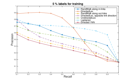
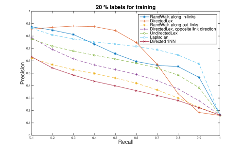
Figure 4: Recall and precision in the WebSpam classification experiment. Each data point shown was computed as an average over 100 runs. The largest standard deviation of the mean precision across the plotted recall values was less than 1.5 %. The algorithm of Zhou et al. [2007] appears as RandWalk (along in-links). We also show RandWalk along out-links. Our directed lex-minimization algorithm appears as DirectedLex. We also show DirectedLex with link directions reversed, along with UndirectedLex and Laplacian.

Appendix D $l_{0}$-Vertex Regularization Proofs

In this appendix, we prove Theorem 7.1 and Theorem 7.2. For the purposes of proving the second theorem, we introduce an alternative version of problem (3). The optimization problem here requires us to minimize $l_{0}$-regularization budget required to obtain an inf-minimizer with gradient below a given threshold:

$$\min_{v\in{\rm I\kern-2.0ptR}^{n}}\,\,\left\|v(T)-v_{0}(T)\right\|_{0}$$ (6)

$$\text{subject to }\left\|\mathsf{grad}_{G}[v]\right\|_{\infty}\leq\alpha.$$

We will also need the following graph construction.

Definition D.1

The $\alpha$-pressure terminal graph of a partially-labeled graph $(G,v_{0})$ is a directed unweighted graph $G_{\alpha}=(T(v_{0}),{\widehat{{E}}})$ such that $(s,t)\in{\widehat{{E}}}$ if and only if there is a terminal path $P$ from $s$ to $t$ in $G$ with

$$\nabla P(v_{0})>\alpha.$$

Note that the $\alpha$-pressure terminal graph has $O(n)$ vertices but may be dense, even when $G$ is not.

Algorithm 13: Algorithm Term-Pressure: Given a well-posed instance $(G,v_{0})$ and $\alpha\geq 0$, outputs $\alpha$ pressure terminal graph $G_{\alpha}$. Initialize $G_{\alpha}$ with vertex set $V_{\alpha}=T(v_{0})$ and edge set ${\widehat{{E}}}=\emptyset$. for each terminal $s\in T(v_{0})$ 1. Compute the distances to every other terminal $t$ by running Dijktra’s algorithm, allowing shortest paths that run through other terminals. 2. Use the resulting distances to check for every other terminal $t$ if there is a terminal path $P$ from $s$ to $t$ with $\nabla P(v_{0})>\alpha$. If there is, add edge $(s,t)$ to ${\widehat{{E}}}$.

Lemma D.2

The $\alpha$-pressure terminal graph of a voltage problem $(G,v_{0})$ can be computed in $O((m+n\log n)n)$ time using algorithm Term-Pressure (Algorithm 13).

• Proof:   The correctness of the algorithm follows from the fact that Dijkstra’s algorithm will identify all shortest distances between the terminals, and the pressure check will ensure that terminal pairs $(s,t)$ are added to ${\widehat{{E}}}$ if and only if they are the endpoints of a terminal path $P$ with $\nabla P(v_{0})>\alpha$. The running time is dominated by performing Dijkstra’s algorithm once for each terminal. A single run of Dijkstra’s algorithm takes $O(m+n\log n)$ time, and this is performed at most $n$ times, for a total running time of $O((m+n\log n)n)$. $\Box$

We make three observations that will turn out to be crucial for proving Theorems 7.1 and 7.2.

Observation D.3

$G_{\alpha}$ is a subgraph of $G_{\beta}$ for $\alpha\geq\beta$.

• Proof:   Suppose edge $(s,t)$ appears in $G_{\alpha}$, then for some path $P$

  $$\nabla P(v_{0})>\alpha\geq\beta,$$

  so the edge also appears in $G_{\beta}$. $\Box$

Observation D.4

$G_{\alpha}$ is transitively closed.

• Proof:   Suppose edges $(s,t)$ and $(t,r)$ appear in $G_{\alpha}$. Let $P_{(s,t)}$, $P_{(t,r)}$, $P_{(s,r)}$ be the respective shortest paths in $G$ between these terminal pairs. Then

  $$\nabla P_{(s,r)}(v_{0})=\frac{v_{0}(s)-v_{0}(r)}{\ell(P_{(s,r)})}\geq\frac{v_{0}(s)-v_{0}(r)}{\ell(P_{(s,t)})+\ell(P_{(t,r)})}=\frac{v_{0}(s)-v_{0}(t)+v_{0}(t)-v_{0}(r)}{\ell(P_{(s,t)})+\ell(P_{(t,r)})}$$ (7)

  $$\geq\min\left(\frac{v_{0}(s)-v_{0}(t)}{\ell(P_{(s,t)})},\frac{v_{0}(t)-v_{0}(r)}{\ell(P_{(t,r)})}\right)>\alpha.$$

  So edge $(s,r)$ also appears in $G_{\alpha}$. This is sufficient for $G_{\alpha}$ to be transitively closed. $\Box$

Observation D.5

$G_{\alpha}$ is a directed acyclic graph.

• Proof:   Suppose for a contradiction that a directed cycle appears in $G_{\alpha}$. Let $s$ and $t$ be two vertices in this cycle. Let $P_{(s,t)}$ and $P_{(t,s)}$ be the respective shortest paths in $G$ between these terminal pairs. Because $G_{\alpha}$ is transitively closed, both edges $(s,t)$ and $(t,s)$ must appear in $G_{\alpha}$. But $(s,t)\in{\widehat{{E}}}$ implies

  $$v_{0}(s)-v_{0}(t)>\alpha\ell(P_{(s,t)})>0,$$

  and similarly $(t,s)\in{\widehat{{E}}}$ implies

  $$v_{0}(t)-v_{0}(s)>\alpha\ell(P_{(t,s)})>0.$$

  This is a contradiction. $\Box$

The usefulness of the $\alpha$-pressure terminal graph is captured in the following lemma. We define a vertex cover of a directed graph to be a vertex set that constitutes a vertex cover in the same graph with all edges taken to be undirected.

Lemma D.6

Given a partially-labeled graph $(G,v_{0})$ and a set $U\subseteq V$, there exists a voltage assignment $v\in{\rm I\kern-2.0ptR}^{n}$ that satisfies

$$\left\{t\in T(v_{0})\mathrel{\mathop{\mathchar 58\relax}}v(t)\neq v_{0}(t)\right\}\subseteq U\text{ and }\left\|\mathsf{grad}_{G}[v]\right\|_{\infty}\leq\alpha,$$

if and only if $U$ is a vertex cover in the $\alpha$-pressure terminal graph $G_{\alpha}$ of $(G,v_{0})$.

• Proof:   We first show the “only if” direction. Suppose for a contradiction that there exists a voltage assignment $v$ for which $\left\|\mathsf{grad}_{G}[v]\right\|_{\infty}\leq\alpha$, but $U$ is not a vertex cover in $G_{\alpha}$. Let $(s,t)$ be an edge $G_{\alpha}$ which is not covered by $U$. The presence of this edge in $G_{\alpha}$ implies that there exists a terminal path $P$ from $s$ to $t$ in $G$ for which

  $$\nabla P(v_{0})>\alpha.$$

  But, by Lemma 3.5 this means there is no assignment $v$ for $G$ which agrees with $v_{0}$ on $s$ and $t$ and has $\left\|\mathsf{grad}_{G}[v]\right\|_{\infty}\leq\alpha$. This contradicts our assumption.

  Now we show the “if” direction. Consider an arbitrary vertex cover $U$ of $G_{\alpha}$. Suppose for a contradiction that there does not exist a voltage assignment $v$ for $G$ with $\left\|\mathsf{grad}_{G}[v]\right\|_{\infty}\leq\alpha$ and $\left\{t\in T(v_{0})\mathrel{\mathop{\mathchar 58\relax}}v(t)\neq v_{0}(t)\right\}\subseteq U$. Define a partial voltage assignment $v_{U}$ given by

  $$v_{U}(t)=\begin{cases}v_{0}(t)&\text{ if }t\in T(v_{0})\setminus U\\ *&\text{ o.w. }\end{cases}$$

  The preceding statement is equivalent to saying that there is no $v$ that extends $v_{U}$ and has $\left\|\mathsf{grad}_{G}[v]\right\|_{\infty}\leq\alpha$. By Lemma 3.5, this means there is terminal path between $s,t\in T(v_{U})$ with gradient strictly larger than $\alpha$. But this means an edge $(s,t)$ is present in $G_{\alpha}$ and is not covered. This contradicts our assumption that $U$ is a vertex cover. $\Box$

We are now ready to prove Theorem 7.2.

• Proof of Theorem 7.2:   We describe and prove the algorithm Outlier. The algorithm will reduce problem (3) to problem (6): Suppose $v^{*}$ is an optimal assignment for problem (3). It achieves a maximum gradient $\alpha^{*}=\left\|\mathsf{grad}_{G}[v^{*}]\right\|_{\infty}$. Using Dijkstra’s algorithm we compute the pairwise shortest distances between all terminals in $G$. From these distances and the terminal voltages, we compute the gradient on the shortest path between each terminal pair. By Lemma 3.5, $\alpha^{*}$ must equal one of these gradients. So we can solve problem (3) by iterating over the set of gradients between terminals and solving problem (6) for each of these $O(n^{2})$ gradients. Among the assignments with $\left\|v(T)-v_{0}(T)\right\|_{0}\leq k$, we then pick the solution that minimizes $\left\|\mathsf{grad}_{G}[v]\right\|_{\infty}$.

  In fact, we can do better. By Observation D.3, $G_{\alpha}$ is a subgraph of $G_{\beta}$ for $\alpha\geq\beta$. This means a vertex cover of $G_{\alpha}$ is also a vertex cover of $G_{\beta}$, and hence the minimum vertex cover for $G_{\beta}$ is at least as large as the minimum vertex cover for $G_{\alpha}$. This means we can do a binary search on the set of $O(n^{2})$ terminal gradients to find the minimum gradient for which there exists an assignment with $\left\|v(T)-v_{0}(T)\right\|_{0}\leq k$. This way, we only make $O(\log n)$ calls to problem (6), in order to solve problem (3).

  We use the following algorithm to solve problem (6). 1. Compute the $\alpha$-pressure terminal graph $G_{\alpha}$ of $G$ using the algorithm Term-Pressure. 2. Compute a minimum vertex cover $U$ of $G_{\alpha}$ using the algorithm Konig-Cover from Theorem 7.3. 3. Define a partial voltage assignment $v_{U}$ given by $$v_{U}(t)=\begin{cases}v_{0}(t)&\text{ if }t\in T(v_{0})\setminus U,\\ *&\text{ otherwise.}\end{cases}$$ 4. Using Algorithm 5, compute voltages $v$ that extend $v_{U}$ and output $v$.

  From Lemma D.2, it follows that step 1 computes the $\alpha$-pressure terminal graph in polynomial time. From Theorem 7.3 it follows that step 2 computes the a minimum vertex cover of the $\alpha$-pressure terminal graph in polynomial time, because our observations D.4 and D.5 establish that the graph is a TC-DAG. From Lemma D.6 and Theorem 4.6, it follows that the output voltages solve program (6).

  $\Box$

To prove Theorem 7.1, we use the standard greedy approximation algorithm for MIN-VC (Vazirani [2001]).

Theorem D.7

2-Approximation Algorithm for Vertex Cover. The following algorithm gives a 2-approximation to the Minimum Vertex Cover problem on a graph $G=(V,E)$. 0. Initialize $U=\emptyset$. 1. Pick an edge $(u,v)\in E$ that is not covered by $U$. 2. Add $u$ and $v$ to the set $U$. 3. Repeat from step 1 if there are still edges not covered by $U$. 4. Output $U$.

We are now in a position to prove Theorem 7.1

• Proof of Theorem 7.1:   Given an arbitrary $k$ and a partially-labeled graph $(G,v_{0})$, let $\alpha^{*}$ be the optimum value of program (3). Observe that by Lemma D.6, this implies that $G_{\alpha^{*}}$ has a vertex cover of size $k$. Given the partial assignment $v_{0}$, for every vertex set $U$, we define

  $$v_{U}(t)=\begin{cases}v_{0}(t)&\text{ if }t\in T(v_{0})\setminus U\\ *&\text{ o.w. }\end{cases}$$

  We claim the following algorithm Approx-Outlier  outputs a voltage assignment $v$ with $\left\|\mathsf{grad}_{G}[v]\right\|_{\infty}\leq\alpha^{*}$ and $\left\|v(T)-v_{0}(T)\right\|_{0}\leq 2k$.

  Algorithm Approx-Outlier: 0. Initialize $U=\emptyset$. 1. Using the algorithm SteepestPath (Algorithm 7), find a steepest terminal path in $G$ w.r.t. $v_{U}$. Denote this path $P$ and let $s$ and $t$ be its terminal endpoints. If there is no terminal path with positive gradient, skip to step 4. 2. Add $s$ and $t$ to the set $U$. 3. If $\left|U\right|\leq 2k-2$ then repeat from step 1. 4. Using the algorithm CompInfMin (Algorithm 5), compute voltages $v$ that extend $v_{U}$ and output $v$.

  From the stopping conditions, it is clear that $\left|U\right|\leq 2k$. If in step 1 we ever find that no terminal paths have positive gradient then our $v$ that extends $v_{U}$ will have $\left\|\mathsf{grad}_{G}[v]\right\|_{\infty}=0\leq\alpha^{*}$, by Lemma 3.5. Similarly if we find a steepest path with gradient less than $\alpha^{*}$ w.r.t. $v_{U}$, then for this $U$ there exists $v$ that extends $v_{U}$ and has $\left\|\mathsf{grad}_{G}[v]\right\|_{\infty}\leq\alpha^{*}$. This will continue to hold when if we add vertices to $U$. Therefore, for the final $U$, there will exist an $v$ that extends $v_{U}$ and has $\left\|\mathsf{grad}_{G}[v]\right\|_{\infty}\leq\alpha^{*}$.

  If we never find a steepest terminal path $P$ with $\nabla P(v_{0})\leq\alpha^{*}$, then each steepest path we find corresponds to an edge in $G_{\alpha^{*}}$ that is not yet covered by $U$ and our algorithm in fact implements the greedy approximation algorithm for vertex cover described in Theorem D.7. This implies that the final $U$ is a vertex cover of $G_{\alpha^{*}}$ of size at most $2k$. By Lemma D.6, this implies that there exists a voltage assignment $u$ extending $v_{U}$ that has $\left\|\mathsf{grad}_{G}[u]\right\|_{\infty}\leq\alpha^{*}$. This implies by Theorem 4.6 that the $v$ we output has $\left\|\mathsf{grad}_{G}[v]\right\|_{\infty}\leq\alpha^{*}$.

  In all cases, the $v$ we output extends $v_{U}$, so $\left\|v(T)-v_{0}(T)\right\|_{0}\leq\left|U\right|\leq 2k$. $\Box$

Appendix E Proof of Hardness of $l_{0}$ regularization for $l_{2}$

We will prove Theorem 7.4, by a reduction from minimum bisection. To this end, let $G=(V,E)$ be any graph. We will reduce the minimum bisection problem on $G$ to our regularization problem. Let $n=\left|V\right|$. The graph on which we will perform regularization will have vertex set

$$V\cup{\widehat{{V}}},$$

where ${\widehat{{V}}}$ is a set of $n$ vertices that are in $1$-to-$1$ correspondence with $V$. We assume that every edge in $G$ has weight $1$. We now connect every vertex in ${\widehat{{V}}}$ to the corresponding vertex in $V$ by an edge of weight $B$, for some large $B$ to be determined later. We also connect all of the vertices in ${\widehat{{V}}}$ to each other by edges of weight $B^{3}$. So, we have a complete graph of weight $B^{3}$ edges on ${\widehat{{V}}}$, a matching of weight $B$ edges connecting ${\widehat{{V}}}$ to $V$, and the original graph $G$ on $V$. The input potential function will be

$$v(a)=\begin{cases}0&\text{for $a\in{\widehat{{V}}}$, and}\\ 1&\text{for $a\in V$.}\end{cases}$$

Now set $k=n/2$. We claim that we will be able to determine the value of the minimum bisection from the solution to the regularization problem.

If $S$ is the set of vertices on which $v$ and $w$ differ, then we know that the $w$ is harmonic on $S$: for every $a\in S$, $w(a)$ is the weighted average of the values at its neighbors. In the following, we exploit the fact that $\left|S\right|\leq n/2$.

Claim E.1

For every $a\in S\cap{\widehat{{V}}}$, $w(a)\leq 2/nB^{2}$.

• Proof:   Let $a$ be the vertex in $S\cap{\widehat{{V}}}$ that maximizes $w(a)$. So, $a$ is connected to at least $n/2$ neighbors in ${\widehat{{V}}}$ with $w$-value equal to $0$ by edges of weight $B^{3}$. On the other hand, $a$ has only one neighbor that is not in ${\widehat{{V}}}$, that vertex has $w$-value at most $1$, and it is connected to that vertex by an edge of weight $B$. Call that vertex $c$. We have

  $$((n-1)B^{3}+B)w(a) =Bw(c)+\sum_{b\in{\widehat{{V}}},b\not=a}B^{3}w(b)$$

  $$=Bw(c)+\sum_{b\in{\widehat{{V}}}\cap S,b\not=a}B^{3}w(b)+\sum_{b\in{\widehat{{V}}}-S}B^{3}w(b)$$

  $$\leq B+\sum_{b\in{\widehat{{V}}}\cap S,b\not=a}B^{3}w(a)$$

  $$\leq B+(n/2-1)B^{3}w(a).$$

  Subtracting $(n/2-1)B^{3}w(a)$ from both sides gives

  $$((n/2)B^{3}+B)w(a)\leq B,$$

  which implies the claim. $\Box$

Claim E.2

For $a\in S\cap V$, $w(a)\leq n/B$.

• Proof:   Vertex $a$ has exactly one neighbor in ${\widehat{{V}}}$. Let’s call that neighbor $c$. We know that $w(c)\leq 2/B^{2}n$. On the other hand, vertex $a$ has fewer than $n-1$ neighbors in $V$, and each of these have $w$-value at most $1$. Let $d_{a}$ denote the degree of $a$ in $G$. Then,

  $$(B+d_{a})w(a) \leq d_{a}+B\frac{2}{B^{2}n}.$$

  So,

  $$w(a) \leq\frac{d_{a}+2/Bn}{d_{a}+B}$$

  $$\leq\frac{n+(2/Bn)}{B+n}$$

  $$\leq n/B.$$

  $\Box$

We now estimate the value of the regularized objective function. To this end, we assume that

$$\left|S\right|=k=n/2.$$

Let

$$T=S\cap V,$$

and

$$t=\left|T\right|.$$

We will prove that $S\subset V$ and so $S=T$ and $t=n/2$.

Let $\delta$ denote the number of edges on the boundary of $T$ in $V$. Once we know that $t=n/2$, $\delta$ is the size of a bisection.

Claim E.3

The contribution of the edges between $V$ and ${\widehat{{V}}}$ to the objective function is at least

$$(n-t)B-4/B$$

and at most

$$(n-t)B+tn^{2}/B.$$

• Proof:   For the lower bound, we just count the edges between vertices in $V\setminus T$ and ${\widehat{{V}}}$. There are $n-t$ of these edges, and each of them has weight $B$. The endpoint in $V\setminus T$ has $w$-value $1$, and the endpoint in ${\widehat{{V}}}$ has $w$-value at most $2/nB^{2}$. So, the contribution of these edges is at least

  $$(n-t)B(1-2/nB^{2})^{2}\geq(n-t)B(1-4/nB^{2})\geq(n-t)B-4/B.$$

  For the upper bound, we observe that the difference in $w$-values across each of these $n-t$ edges is at most $1$, so their total contribution is at most

  $$(n-t)B.$$

  Since for every vertex $a\in T$, $w(a)\leq n/B$, and also every vertex $b\in{\widehat{{V}}}$, $w(b)\leq 2/nB^{2}$, the contribution due to edges between $T$ and ${\widehat{{V}}}$ is at most

  $$t(n/B)^{2}B=tn^{2}/B.$$

  $\Box$

We will see that this is the dominant term in the objective function. The next-most important term comes from the edges in $G$.

Claim E.4

The contribution of the edges in $G$ to the objective function is at least

$$\delta(1-2n/B)$$

and at most

$$\delta+(t^{2}/2)(n/B)^{2}$$

• Proof:   Let $(a,b)\in E$. If neither $a$ nor $b$ is in $T$, then $w(a)=w(b)=1$, and so this edge has no contribution. If $a\in T$ but $b\not\in T$, then the difference in $w$-values on them is between $(1-n/B)$ and $1$. So, the contribution of such edges to the objective function is between

  $$\delta(1-2n/B)\text{ and }\delta.$$

  Finally, if $a$ and $b$ are in $T$, then the difference in $w$-values on them is at most $n/B$, and so the contribution of all such edges to the objective function is at most

  $$(t^{2}/2)(n/B)^{2}.$$

  $\Box$

Claim E.5

The edges between pairs of vertices in ${\widehat{{V}}}$ contribute at most $2/B$ to the objective function.

• Proof:   As $0\leq w(a)\leq 2/B^{2}n$ for every $a\in{\widehat{{V}}}$, every edge between two vertices in ${\widehat{{V}}}$ can contribute at most

  $$B^{3}(2/B^{2}n)^{2}=4/Bn^{2}.$$

  As there are fewer than $n^{2}/2$ such edges, their total contribution to the objective function is at most

  $$(n^{2}/2)(4/Bn^{2})=2/B.$$

  $\Box$

Lemma E.6

If $n\geq 4$ and $B=2n^{3}$, the value of the objective function is at least

$$(n-t)B+\delta-1/2$$

and at most

$$(n-t)B+\delta+1/3.$$

• Proof:   Summing the contributions in the preceding three claims, we see that the value of the objective function is at least

  $$(n-t)B-4/B+\delta(1-2n/B) \geq(n-t)B+\delta-4/B-2n\delta/B$$

  $$\geq(n-t)B+\delta-n^{3}/B$$

  $$\geq(n-t)B+\delta-1/2,$$

  as $\delta\leq(n/2)^{2}$.

  Similarly, the objective function is at most

  $$(n-t)B+tn^{2}/B+\delta+(t^{2}/2)(n/B)^{2}+2/B \leq(n-t)B+n^{3}/2B+\delta+n^{4}/8B^{2}+2/B$$

  $$\leq(n-t)B+n^{3}/2B+\delta+1/32n^{2}+1/n^{3}$$

  $$\leq(n-t)B+\delta+1/3.$$

  $\Box$

Claim E.7

If $n\geq 2$ and $B=2n^{3}$, then $S\subset V$.

• Proof:   The objective function is minimized by making $t$ as large as possible, so $t=n/2$ and $S\subset V$. $\Box$

Theorem E.8

The value of the objective function reveals the value of the minimum bisection in $G$.

• Proof:   The value of the objective function will be between

  $$(n/2)B+\delta-1/2$$

  and

  $$(n/2)B+\delta+1/3.$$

  So, the objective function will be smallest when $\delta$ is as small as possible. $\Box$

Theorem E.8 immediately implies Theorem 7.4.

References

• Alamgir and Luxburg [2011] Morteza Alamgir and Ulrike V. Luxburg. Phase transition in the family of p-resistances. In Advances in Neural Information Processing Systems 24, pages 379–387. 2011. URL http://books.nips.cc/papers/files/nips24/NIPS2011_0278.pdf.
• Aronsson [1967] Gunnar Aronsson. Extension of functions satisfying lipschitz conditions. Arkiv för Matematik, 6(6):551–561, 1967. ISSN 0004-2080. doi: 10.1007/BF02591928. URL http://dx.doi.org/10.1007/BF02591928.
• Aronsson et al. [2004] Gunnar Aronsson, Michael G. Crandall, and Petri Juutinen. A tour of the theory of absolutely minimizing functions. Bull. Amer. Math. Soc. (N.S.), 41(4):439–505, 2004. ISSN 0273-0979. doi: 10.1090/S0273-0979-04-01035-3. URL http://dx.doi.org/10.1090/S0273-0979-04-01035-3.
• Barles and Busca [2001] Guy Barles and Jérôme Busca. Existence and comparison results for fully nonlinear degenerate elliptic equations without zeroth-order term. Comm. Partial Differential Equations, 26:2323–2337, 2001.
• Belkin et al. [2004] Mikhail Belkin, Irina Matveeva, and Partha Niyogi. Regularization and semi-supervised learning on large graphs. In Learning Theory, volume 3120 of Lecture Notes in Computer Science, pages 624–638. Springer Berlin Heidelberg, 2004. ISBN 978-3-540-22282-8. doi: 10.1007/978-3-540-27819-1˙43. URL http://dx.doi.org/10.1007/978-3-540-27819-1_43.
• Bridle and Zhu [2013] Nick Bridle and Xiaojin Zhu. $p$-voltages: Laplacian regularization for semi-supervised learning on high-dimensional data. In Eleventh Workshop on Mining and Learning with Graphs (MLG2013), 2013.
• Castillo et al. [2006] Carlos Castillo, Debora Donato, Luca Becchetti, Paolo Boldi, Stefano Leonardi, Massimo Santini, and Sebastiano Vigna. A reference collection for web spam. SIGIR Forum, 40(2):11–24, December 2006. ISSN 0163-5840. doi: 10.1145/1189702.1189703. URL http://doi.acm.org/10.1145/1189702.1189703.
• Chapelle et al. [2010] Olivier Chapelle, Bernhard Schlkopf, and Alexander Zien. Semi-Supervised Learning. The MIT Press, 1st edition, 2010. ISBN 0262514125, 9780262514125.
• Cohen et al. [2014] Michael B Cohen, Rasmus Kyng, Gary L Miller, Jakub W Pachocki, Richard Peng, Anup B Rao, and Shen Chen Xu. Solving SDD linear systems in nearly $m\log^{1/2}n$ time. In Proceedings of the 46th Annual ACM Symposium on Theory of Computing, pages 343–352. ACM, 2014.
• Crandall et al. [2001] M.G. Crandall, L.C. Evans, and R.F. Gariepy. Optimal lipschitz extensions and the infinity laplacian. Calculus of Variations and Partial Differential Equations, 13(2):123–139, 2001. ISSN 0944-2669. doi: 10.1007/s005260000065. URL http://dx.doi.org/10.1007/s005260000065.
• Daitch and Spielman [2008] Samuel I. Daitch and Daniel A. Spielman. Faster approximate lossy generalized flow via interior point algorithms. In Proceedings of the Fortieth Annual ACM Symposium on Theory of Computing, STOC ’08, pages 451–460, New York, NY, USA, 2008. ACM. ISBN 978-1-60558-047-0. doi: 10.1145/1374376.1374441. URL http://doi.acm.org/10.1145/1374376.1374441.
• Egger and Huotari [1990] Alan Egger and Robert Huotari. Rate of convergence of the discrete polya algorithm. Journal of Approximation Theory, 60(1):24 – 30, 1990. ISSN 0021-9045. doi: http://dx.doi.org/10.1016/0021-9045(90)90070-7. URL http://www.sciencedirect.com/science/article/pii/0021904590900707.
• Fefferman [2009a] Charles Fefferman. Whitney’s extension problems and interpolation of data. Bull. Amer. Math. Soc. (N.S.), 46(2):207–220, 2009a. ISSN 0273-0979. doi: 10.1090/S0273-0979-08-01240-8. URL http://dx.doi.org/10.1090/S0273-0979-08-01240-8.
• Fefferman [2009b] Charles Fefferman. Fitting a [image] -smooth function to data, iii. Annals of Mathematics, 170(1):pp. 427–441, 2009b. ISSN 0003486X. URL http://www.jstor.org/stable/40345469.
• Fefferman and Klartag [2009] Charles Fefferman and Bo’az Klartag. Fitting a cm -smooth function to data i. Annals of Mathematics, 169(1):pp. 315–346, 2009. ISSN 0003486X. URL http://www.jstor.org/stable/40345445.
• Fulkerson [1956] D. R. Fulkerson. Note on dilworths decomposition theorem for partially ordered sets. Proc. Amer. Math. Soc, 1956.
• Gaffney and Powell [1976] P.W. Gaffney and M.J.D. Powell. Optimal interpolation. In Numerical Analysis, volume 506 of Lecture Notes in Mathematics, pages 90–99. Springer Berlin Heidelberg, 1976. ISBN 978-3-540-07610-0. doi: 10.1007/BFb0080117. URL http://dx.doi.org/10.1007/BFb0080117.
• Gottlieb et al. [2013] L.-A. Gottlieb, A. Kontorovich, and R. Krauthgamer. Efficient classification for metric data. CoRR, abs/1306.2547, 2013. URL http://arxiv.org/abs/1306.2547.
• Gottlieb et al. [2013b] L.-A. Gottlieb, A. Kontorovich, and R. Krauthgamer. Efficient regression in metric spaces via approximate lipschitz extension. In Similarity-Based Pattern Recognition, volume 7953 of Lecture Notes in Computer Science, pages 43–58. Springer Berlin Heidelberg, 2013b. ISBN 978-3-642-39139-2. doi: 10.1007/978-3-642-39140-8˙3. URL http://dx.doi.org/10.1007/978-3-642-39140-8_3.
• Jensen [1993] Robert Jensen. Uniqueness of lipschitz extensions: Minimizing the sup norm of the gradient. Archive for Rational Mechanics and Analysis, 123(1):51–74, 1993. ISSN 0003-9527. doi: 10.1007/BF00386368. URL http://dx.doi.org/10.1007/BF00386368.
• Kirszbraun [1934] M. Kirszbraun. Über die zusammenziehende und lipschitzsche transformationen. Fundamenta Mathematicae, 22(1):77–108, 1934. URL http://eudml.org/doc/212681.
• Lazarus et al. [1999] Andrew J. Lazarus, Daniel E. Loeb, James G. Propp, Walter R. Stromquist, and Daniel H. Ullman. Combinatorial games under auction play. Games and Economic Behavior, 27(2):229 – 264, 1999. ISSN 0899-8256. doi: http://dx.doi.org/10.1006/game.1998.0676. URL http://www.sciencedirect.com/science/article/pii/S0899825698906765.
• Ma and Fu [2011] Yunqian Ma and Yun Fu. Manifold Learning Theory and Applications. CRC Press, Inc., Boca Raton, FL, USA, 1st edition, 2011. ISBN 1439871094, 9781439871096.
• McShane [1934] E. J. McShane. Extension of range of functions. Bull. Amer. Math. Soc., 40(12):837–842, 12 1934. URL http://projecteuclid.org/euclid.bams/1183497871.
• Micchelli et al. [1976] C.A. Micchelli, T.J. Rivlin, and S. Winograd. The optimal recovery of smooth functions. Numerische Mathematik, 26(2):191–200, 1976. ISSN 0029-599X. doi: 10.1007/BF01395972. URL http://dx.doi.org/10.1007/BF01395972.
• Milman [1999] V. A. Milman. Absolutely minimal extensions of functions on metric spaces. 1999. URL http://iopscience.iop.org/1064-5616/190/6/A05/pdf/MSB_190_6_A05.pdf.
• Nadler et al. [2009] Boaz Nadler, Nathan Srebro, and Xueyuan Zhou. Statistical analysis of semi-supervised learning: The limit of infinite unlabelled data. 2009. URL http://ttic.uchicago.edu/~nati/Publications/NSZnips09.pdf.
• Naor and Sheffield [2010] A. Naor and S. Sheffield. Absolutely minimal Lipschitz extension of tree-valued mappings. CoRR, abs/1005.2535, May 2010. URL http://arxiv.org/abs/1005.2535.
• Oberman [2011] A. M. Oberman. Finite difference methods for the Infinity Laplace and p-Laplace equations. CoRR, abs/1107.5278, July 2011. URL http://arxiv.org/abs/1107.5278.
• Peres et al. [2011] Yuval Peres, Oded Schramm, Scott Sheffield, and DavidB. Wilson. Tug-of-war and the infinity laplacian. In Selected Works of Oded Schramm, Selected Works in Probability and Statistics, pages 595–638. Springer New York, 2011. ISBN 978-1-4419-9674-9. doi: 10.1007/978-1-4419-9675-6˙18. URL http://dx.doi.org/10.1007/978-1-4419-9675-6_18.
• Sheffield and Smart [2010] S. Sheffield and C. K. Smart. Vector-valued optimal Lipschitz extensions. CoRR, abs/1006.1741, June 2010. URL http://arxiv.org/abs/1006.1741.
• Sinop and Grady [2007] Ali Kemal Sinop and Leo Grady. A seeded image segmentation framework unifying graph cuts and random walker which yields a new algorithm. In Computer Vision, 2007. ICCV 2007. IEEE 11th International Conference on, pages 1–8. IEEE, 2007.
• Vazirani [2001] Vijay V. Vazirani. Approximation Algorithms. Springer-Verlag New York, Inc., New York, NY, USA, 2001. ISBN 3-540-65367-8.
• von Luxburg and Bousquet [2003] Ulrike von Luxburg and Olivier Bousquet. Distance-based classification with lipschitz functions. In Learning Theory and Kernel Machines, volume 2777 of Lecture Notes in Computer Science, pages 314–328. Springer Berlin Heidelberg, 2003. ISBN 978-3-540-40720-1. doi: 10.1007/978-3-540-45167-9˙24. URL http://dx.doi.org/10.1007/978-3-540-45167-9_24.
• Whitney [1934] Hassler Whitney. Analytic extensions of differentiable functions defined in closed sets. Transactions of the American Mathematical Society, 36(1):pp. 63–89, 1934. ISSN 00029947. URL http://www.jstor.org/stable/1989708.
• Zhou et al. [2007] Dengyong Zhou, Christopher J. C. Burges, and Tao Tao. Transductive link spam detection. In Proceedings of the 3rd International Workshop on Adversarial Information Retrieval on the Web, AIRWeb ’07, pages 21–28, New York, NY, USA, 2007. ACM. ISBN 978-1-59593-732-2. doi: 10.1145/1244408.1244413. URL http://doi.acm.org/10.1145/1244408.1244413.
• Zhu et al. [2003] Xiaojin Zhu, Zoubin Ghahramani, and John Lafferty. Semi-supervised learning using gaussian fields and harmonic functions. In IN ICML, pages 912–919, 2003.