Probabilistic Object Tracking using a Range Camera

Abstract

We address the problem of tracking the 6-DoF pose of an object while it is being manipulated by a human or a robot. We use a dynamic Bayesian network to perform inference and compute a posterior distribution over the current object pose. Depending on whether a robot or a human manipulates the object, we employ a process model with or without knowledge of control inputs. Observations are obtained from a range camera. As opposed to previous object tracking methods, we explicitly model self-occlusions and occlusions from the environment, e.g, the human or robotic hand. This leads to a strongly non-linear observation model and additional dependencies in the Bayesian network. We employ a Rao-Blackwellised particle filter to compute an estimate of the object pose at every time step. In a set of experiments, we demonstrate the ability of our method to accurately and robustly track the object pose in real-time while it is being manipulated by a human or a robot.

100mm(.-10.3cm) 2013 IEEE/RSJ International Conference on
Intelligent Robots and Systems (IROS)
November 3-7, 2013. Tokyo, Japan

I INTRODUCTION

Manipulation of objects is one of the remaining key challenges of robotics. In recent years, tremendous progress has been made in the area of data-driven grasp synthesis [2]. Given an object, the goal is to infer a suitable grasp that adheres certain properties, e.g. stability or functionality. In many cases, this grasp is then performed in an open-loop manner without taking any feedback into account, e.g. in [18, 1, 4]. This approach can lead to a very poor success rate especially in the presence of noisy and incomplete sensor data, inaccurate models, or in a dynamic environment. We have recently shown that the robustness of grasp execution can be greatly increased by continuously taking tactile sensor feedback into account [14]. This enables the robot to adapt to unforeseen situations.

In this paper, we use visual sensing to continuously track the 6-DoF pose of an object during manipulation, which could enable the robot to adapt its actions according to the perceived state of the environment. In contrast to our previous work [14], such adaptation would not rely on being in contact with the object. Visual tracking is also crucial for precision manipulation tasks such as drilling a hole or inserting a key into a lock [17]. These tasks require precise alignment of a tool in the robot hand with objects in the environment.

We present a real-time marker-less object tracking algorithm as a basis for these kinds of systems. We consider the movement of an object as a stochastic process and model it in a dynamic Bayesian network. We perform inference in this network to compute a posterior distribution over the current object pose. We follow the general paradigm of a Bayes filter [19] in which we (i) predict the current object pose given the previous pose and then (ii) update the prediction given an observation. For the first step, we use a process model that can either be dependent on control inputs (in case the robot is moving the object) or be based on the simple assumption that the object pose will not change significantly in a short time (in case the object is not being held by the robot).

Figure 1: The robot is tracking an impact wrench (left image) in real-time using a depth sensor (red object model in the right image). Fiducial markers are used for baseline comparison only.

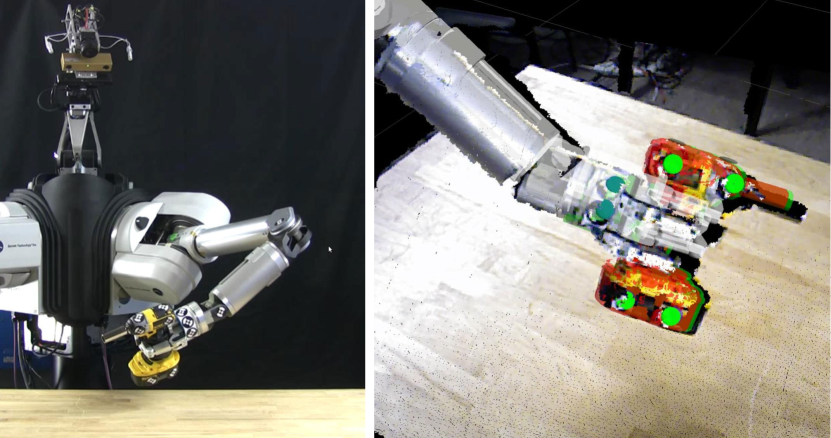
We use a range camera to obtain dense depth images of the scene. For the update step, we develop an observation model that, given the current estimate of the object pose, determines the likelihood of the observed depth data. We explicitly model self-occlusions and occlusions from the environment. Therefore, the algorithm becomes more robust to these effects. However, the observation model is strongly non-linear and new dependencies are introduced in the Bayes network. We therefore employ a Rao-Blackwellised particle filter [5] to compute a posterior distribution over the current object pose.

The paper is structured as follows. In the next section, we review existing approaches to object tracking, especially in the context of robotic manipulation. We then briefly review the Bayes filter and associated inference methods in Sect. III. In Sect. IV and V the observation and process models are derived. In Sect. VI we formulate the proposed algorithm. Experimental results are presented in Sect. VII. Finally, we conclude and present ideas for future work in Sect. VIII.

II RELATED WORK

Existing approaches to real-time 6-DoF pose tracking can be divided into two groups according to the type of data used. The first group consists of algorithms which mainly rely on 2D images, e.g. [7, 11, 3]. This kind of approaches may be sensitive to the amount of texture on the tracked object and in the scene as well as to lightning conditions. It has been shown that using depth data can add robustness to tasks such as SLAM [13], object detection and recognition [12, 9]. Therefore it is worth exploring the second group of methods for 6 DoF pose tracking that rely on range data. In this section, we review those which aim for real-time performance and use dense depth data as sensory input.

Ren and Reid [16] represent the object surface as the zero level in a level-set embedding function. Specifically, it is based on a truncated 3D distance map. The pose of the object is found by minimizing over the sum of all points in the 3D point cloud back-projected into the object frame and evaluated in the embedding function. Optimization is performed through the Levenberg-Marquardt algorithm. The GPU implementation of this approach performs in real-time. Through the choice of a robust estimator and a robust variant of the 3D distance map it seems to work well even in the presence of heavy occlusions. There are however no experiments provided where an occluding object is in contact with the tracked object. It is not clear how the algorithm would perform in that situation since points from the occluding object might be mistaken for the tracked object. Our method, in contrast, is formulated in a Bayesian framework that allows us to fuse different sources of information in a probabilistic manner, we fuse for example the knowledge of the control inputs with the depth measurements in order to estimate the pose of the object. Furthermore, we explicitly model occlusions in this framework and finally, we obtain a posterior distribution over the pose instead of just a point estimate.

Hebert et al. [8] fuse sensory data from stereo cameras, monocular images and tactile sensors for simultaneously estimating the pose of the object and the robot arm with an Unscented Kalman Filter (UKF). Using all these sensor modalities, the approach allows to track the object well while it is being held by the robot. It is not clear how well it works when the object is not being held by the robot, since in that case less information about the motion is available. Our method uses the knowledge of the control inputs as well, when available, but it is able to track an object even when it is not being held by the robot.

Ueda [20] uses a sampling-based approach. The object is represented as a partial point cloud and tracking is performed using a particle filter. The likelihood of an observation is computed using a function of the squared distance between each point in the object model and its closest point in the observed point cloud, as well as the distance between their respective colors. This approach neither models noise in the sensor nor occlusion. Since in terms of experimental results there is only a video available, it is not clear how well this method performs in general settings.

In contrast to the mentioned algorithms, occlusion is modeled explicitly in our observation model. As we will show in Sect. IV in more detail, this leads to strong non-linearities. We therefore use a sampling-based approach to filter the pose of the object. This has the advantage that even non-Gaussian multi-modal distributions can be represented. The main drawback of sampling-based approaches is that they are computationally expensive. Nevertheless we show in the experimental section that we achieve real time tracking using only one CPU core.

III Bayes Filter

In this section, we briefly discuss the Bayes filter and a number of techniques to perform inference in cases where the problem cannot be solved analytically.

The assumptions made in a Bayes filter are twofold. Firstly, the Markov assumption asserts that each state only depends on the previous state. Secondly, it is assumed that the state is sufficient to predict the (potentially noisy) observation [19].

Figure 2: This graph represents the independence assumptions made by a Bayes filter.

These independence assumptions are represented in a probabilistic graphical model (PGM) in Fig. 2. The goal in state estimation is to find the posterior $p(x_{t}|z_{1:t},u_{1:t})$ over the state $x_{t}$ given all the observations $z_{1:t}$ and the control inputs $u_{1:t}$. There are different approaches for performing inference in this model that depend on the form of the process model $p(x_{t}|x_{t-1},u_{t})$ and the observation model $p(z_{t}|x_{t})$. For a linear process and observation model and each being subject to Gaussian noise, the inference problem can be optimally solved with a Kalman Filter.

If the process and observation model can be approximated as being locally linear and the noise can be assumed to be Gaussian, then an Extended Kalman Filter (EKF) or an Unscented Kalman Filter (UKF) can be used. In the EKF, the process and observation model are linearized to compute the covariance matrix of the current state estimate. In the UKF, samples around the mean of the current state estimate or prediction are drawn and pushed through the non-linear models. The projected samples serve as the base to estimate the Gaussian posterior distribution.

Finally, there are nonparametric methods to solve the inference problem. The most well known is the particle filter which represents the posterior over the state at time $t$, $p(x_{t}|z_{1:t},u_{1:t})$, by a set of samples $\{x_{t}^{(l)}\}$ which are distributed accordingly. Such a set of samples can be obtained by sampling from the distribution over the entire sequence of states $p(x_{1:t}|z_{1:t},u_{1:t})$ and then dropping all the previous states $x_{1:t-1}$. Consequently, the previous states do not have to be marginalized out in a particle filter, we can thus express $p(x_{1:t}|z_{1:t},u_{1:t})$ instead of $p(x_{t}|z_{1:t},u_{1:t})$ [19].

As will be discussed in more detail in Sect. IV, we introduce a variable $o_{t}$ describing which parts of the image are occluded, therefore our state $x_{t}$ consists of the 6-DoF pose and the occlusion $(r_{t},o_{t})$. The posterior distribution $p(x_{1:t}|z_{1:t},u_{1:t})$ can then be written as

$$p(r_{1:t},o_{1:t}|z_{1:t},u_{1:t})=p(o_{1:t}|r_{1:t},z_{1:t},u_{1:t})p(r_{1:t}|z_{1:t},u_{1:t}).$$

As a result of the functional form of our observation model, derived in Sect. IV, and our process model, discussed in Sect. V, the variables $o_{1:t}$ can be marginalized out analytically while the variables $r_{1:t}$ cannot. In a dynamic Bayesian network with these properties, inference can be performed using a Rao-Blackwellised particle filter [5]. Integrating out the previous occlusions $o_{1:t-1}$ we obtain

$$\!\!\!p(r_{1:t},o_{t}|z_{1:t},u_{1:t})\!=\!p(o_{t}|r_{1:t},z_{1:t},u_{1:t})p(r_{1:t}|z_{1:t},u_{1:t})$$ (1)

Since the variables $r_{1:t-1}$ cannot be integrated out analytically, the second term is represented, as in a common particle filter, with a set of samples. In a Rao-Blackwellised particle filter the posterior over the full state $p(r_{t},o_{t}|z_{1:t},u_{1:t})$ is thus represented by a set of particles $r_{1:t}^{(l)}$ distributed according to $p(r_{1:t}|z_{1:t},u_{1:t})$, each associated with a probability $p(o_{t}|r_{1:t}^{(l)},z_{1:t},u_{1:t})$.

Before we apply this method to object tracking we will derive the observation and the process model.

IV OBSERVATION MODEL

The objective is to infer the 6-DoF pose $r_{t}$ of an object assuming that we have a 3D model. The observation model $p(z_{t}|r_{t})$ expresses what depth image we expect to observe given the pose of the object. However, if it is not known whether the object is occluded or not, we cannot predict the depth which should be measured. Therefore, we introduce a set of binary variables $o_{t}=\{o_{t}^{i}\}$ modelling occlusion. $o_{t}^{i}=0$ means that the object is visible at time $t$ in pixel $i$, whereas $o_{t}^{i}=1$ indicates that it is occluded. Thus, the full state $x_{t}=(r_{t},o_{t})$ consists of the 6-DoF pose and the occlusion for each pixel $i$. The graphical model in Fig. 2 can be expanded as shown in Fig. 3.

Figure 3: This graph represents the independence assumptions made by a our filter. The box is a plate which represents the $I$ pixels.

The depth measurements $\{z_{t}^{i}\}$ at each pixel (including the noise) are assumed to be independent given the state. This assumption is reasonable since the pose and the occlusion variables allow us to predict the observation. Furthermore, we assume the occlusions ${o_{t}^{i}}$ of different pixels to be independent. Although we thereby ignore relations between neighboring pixels, inference becomes more efficient as will be described in Sect. VI.

We can now write $p(z_{t}|r_{t},o_{t})=\prod_{i}p(z_{t}^{i}|r_{t},o_{t}^{i})$ as the product of measurement likelihoods at each pixel $i$ given the pose and whether the object is occluded in pixel $i$. By marginalizing out the occlusion variables $p(z_{t}^{i}|r_{t})=\sum_{o_{t}^{i}}p(z_{t}^{i}|r_{t},o_{t}^{i})p(o_{t}^{i})$, we obtain a model which is closely related to beam-based models discussed in robotics literature [19]. These consist of a weighted sum of an observation model assuming that the object is occluded and an observation model assuming that it is visible. The important difference to our approach is that we continuously estimate the probability $p(o_{t}^{i})$ of the object being occluded whereas in [19] this is a parameter which is set off-line and kept constant during execution.

To express the observation model $p(z_{t}^{i}|r_{t},o_{t}^{i})$, we represent the measurement process in Fig. 4, which is a subpart of the graphical model in Fig. 3.

Figure 4: This graph shows the measurement process of the camera. It is a subpart of the graph in Fig. 3, zoomed in on one observation.

Two auxiliary variables $a^{i}$ and $b^{i}$ have been introduced. These variables will be integrated out, but they are convenient for the formulation of the observation model. Since we are looking at only one time step, the time index is omitted here. $a^{i}$ is the distance to the tracked object along the beam defined by pixel $i$ and $b_{i}$ is the distance to the object which is seen in pixel $i$; this might not be the tracked object, depending on whether it is occluded.

We can now describe the process which leads to the observation. Given the pose $r$, we can compute the distance to the tracked object $a^{i}$ for a given pixel $i$. Then given the distance to the tracked object and the information whether it is occluded, we can predict the distance to the object $b^{i}$ seen in pixel $i$, which might or might not be the tracked object. Knowing this distance, it is easy to predict a measurement $z^{i}$. Using the independence assumptions from Fig. 4, this process can be formally written as

$$p(z^{i}|r,o^{i}) =\int_{a,b}p(z^{i}|b^{i})p(b^{i}|a^{i},o^{i})p(a^{i}|r).$$ (2)

In the following, we express each of these terms going from right to left. $p(a^{i}|r)$ is the probability distribution over the distance to the tracked object given the pose. This is simply the distance $d^{i}(r)$ to the intersection of the beam defined by pixel $i$ with the object model in pose $r$. Additionally, there is some noise due to errors in the object model:

$$p(a^{i}|r)=\mathcal{N}(a^{i}|d^{i}(r),\sigma_{m}).$$ (3)

$p(b^{i}|a^{i},o^{i})$ expresses the distance to the object measured in pixel $i$ given the distance to the tracked object and the occlusion. If the $o^{i}=0$ the object is visible, therefore $a^{i}$ and $b^{i}$ have to be identical. Otherwise $b_{i}$ has to be smaller than $a_{i}$, since the occluding object is necessarily in front of the tracked object. Formally we can write this as

$$p(b^{i}|a^{i},o^{i})=\begin{cases}\delta(b^{i}-a^{i})&\!\!\text{if }o^{i}\!=\!0\\ I(b^{i}>0\land b^{i}<a^{i})\frac{\lambda e^{-\lambda b^{i}}}{1-e^{-\lambda a^{i}}}&\!\!\text{if }o^{i}=1\end{cases}$$ (4)

where $I$ is the indicator function which is equal to one if the condition is true and zero otherwise. $\delta$ denotes the Dirac delta function. We assume that the probability of a beam intersecting with an object other than the tracked object is equal for any interval of equal length. This implies that the probability of the beam hitting the first object at a distance $b^{i}$ decays exponentially if the observed object is not the tracked object, see Eq. 4. The parameter $\lambda$ is a function of the half-life, i.e. the distance at which we expect half of the beams to not have intersected with an object yet. The algorithm is not sensitive to this parameter, therefore we simply set the half-life to a number which seems reasonable. In all our experiments we used 1 m.

Finally, we express $p(z^{i}|b^{i})$ which is the distribution over the measurement $z^{i}$ given the distance of the observed object to the camera. The difference in these two quantities is due to noise in the measurement of the range camera. We used an Asus XTION Pro depth sensor in our experiments and thus attempted to model its noise. Khoshelham and Elberink [10] estimated the noise in the depth measurements of a Microsoft Kinect which is based on the same design as the sensor we used. The authors showed that the noise increases with the depth squared. We define the camera standard deviation $\sigma_{c}$ accordingly. Fallon et al. [6] model the noise in the Kinect camera by the sum of a Gaussian distribution and a constant term to shift more weight to the tails than in a purely normal distribution. We also found it to be advantageous to have a heavy tailed distribution and thus define the distribution in a similar fashion as

$$p(z^{i}|b^{i}) \!\!=\!\!(1-\beta)\mathcal{N}(z^{i}|b^{i},\sigma_{c})+\beta\frac{I(z^{i}>0\land z^{i}<m)}{m}$$ (5)

where $I$ is the indicator function and $m$ is the maximum depth which can be measured by the range camera, 6 m in our case. In all our experiments the weight of the tails $\beta$ was set to $0.01$, as proposed in [6] and $\sigma_{c}$ was defined according to [10].

Now the observation model is fully specified. We plot the likelihood of the pose $p(z^{i}|r)=\sum_{o^{i}}p(z^{i}|r,o^{i})p(o^{i})$ in Fig. 5 as a function of the depth measured in pixel $i$, given that the predicted distance to the object $d^{i}(r)$ is equal to 1 m.

Figure 5: This graph shows the probability of an observation given a pose $p(z^{i}|r)=\sum_{o^{i}}p(z^{i}|r,o^{i})p(o^{i})$. The pose $r$ is such that the distance to the object model $d^{i}(r)$ is equal to 1 m. There are five curves for different probabilities of the object being visible $p(o^{i}=0)$.

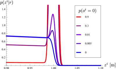
For a small probability of the object being visible the function is almost constant in observed depth $z^{i}$ with a steep decrease at the predicted depth $d^{i}(r)=1$. This intuitively makes sense since the occluding object has to be closer to the camera than the tracked object. As the probability of the object being visible increases, a more and more pronounced spike appears at the predicted depth. At the same time the probability of measuring a depth which is smaller than the predicted depth diminishes as we become more certain that the object is not occluded.

V PROCESS MODELS

The pose process model $p(r_{t}|r_{t-1},u_{t})$ describes how we expect the object pose to change over time given the last pose and the control inputs. The occlusion process model $p(o_{t}^{i}|o_{t-1}^{i})$ describes how the occlusions propagate. In this section we will model these two probability distributions.

V-A Pose Process Model

The process model for the pose $p(r_{t}|r_{t-1},u_{t})$ depends of course on the underlying process. In our experiments we test two different scenarios. In the first case where the object is moved by a human arm, we do thus not have access to the control inputs and therefore simply propagate the pose by a small random rotation and translation drawn from a Gaussian distribution.

In the second case, the object is moved by a robot and we thus make use of the control inputs. From the control inputs, we can compute the expected velocity of the object being held for every time step. Since this velocity is not entirely accurate, we model the noise as being Gaussian in the translational as well as the rotational velocity. When the object is being moved by a robot, the uncertainty is of course much smaller than when it is being moved by a human arm.

V-B Occlusion Process Model

The distribution $p(o_{t}^{i}|o_{t-1}^{i})$ has only two parameters since the variables are binary. We have to determine the probability of the object being visible in pixel $i$ given that it was visible in the last time step, $p(o_{t}^{i}=0|o_{t-1}^{i}=0)$ and the probability that the object is visible given that is was occluded in the last time step $p(o_{t}^{i}=0|o_{t-1}^{i}=1)$. In all our experiments we set $p(o_{t}^{i}=0|o_{t-1}^{i}=0)=0.9$ and $p(o_{t}^{i}=0|o_{t-1}^{i}=1)=0.3$ for a time delta of one second. This represents the fact that if the object was observed in the last time step we expect to observe it again in the current time step. The algorithm proved to not be very sensitive to these parameters, so their values were simply set by hand without any tuning. A more systematic estimation is the subject of future work.

VI FILTERING ALGORITHM

Since we have introduced a new set of variables, we do not only infer the pose of the object $r_{t}$ but also the occlusion $o_{t}$. As can be seen from Fig. 5, our observation model is highly nonlinear and results in a likelihood of the pose $p(z_{t}|r_{t})$ which does not fit well to a normal distribution. With a Gaussian distribution, we can essentially express that a variable should be somewhere close to a certain value. However as discussed in Sect. IV, for the proposed algorithm it is central to also be able to express that a variable should be larger than a certain value. This requirement discards algorithms which approximate the $p(z_{t}|r_{t})$ with a normal distribution such as KF, EKF and UKF. Therefore, we use sampling to solve the inference problem for the pose $r_{t}$. As shown below, marginalizing out the occlusion variables $o_{t}$ is tractable. We can thus perform inference using a Rao-Blackwellised particle filter as described in Sect. III. Rewriting Eq. 1 for convenience, we have

$$\!\!p(r_{1:t},o_{t}|z_{1:t},u_{1:t})\!\!=\!p(o_{t}|r_{1:t},z_{1:t},u_{1:t})p(r_{1:t}|z_{1:t},u_{1:t})$$ (6)

We are mainly interested in the second term which expresses the distribution over the poses given all the measurements and control inputs. As we will see shortly, the estimate of the pose depends on the estimate of the occlusion i.e. the first term in Eq. 6. In the following, we will therefore express these two terms recursively.

From Fig. 3 we can see that the first term in Eq. 6 factorizes as $p(o_{t}|r_{t},z_{1:t},u_{1:t})=\prod_{i}p(o_{t}^{i}|r_{1:t},z_{1:t},u_{1:t})$. Taking the independence assumptions from Fig. 3 into account, we can express each factor in a recursive form.

$$p(o_{t}^{i}|r_{1:t},z_{1:t},u_{1:t})=$$ (7)

$$\frac{\sum_{o_{t-1}^{i}}\!\left[p(z_{t}^{i}|r_{t},o_{t}^{i})p(o_{t}^{i}|o_{t-1}^{i})p(o_{t-1}^{i}|r_{1:t-1},z_{1:t-1},u_{1:t-1})\!\right]}{\sum_{o_{t}^{i},o_{t-1}^{i}}\!\!\!\left[p(z_{t}^{i}|r_{t},o_{t}^{i})p(o_{t}^{i}|o_{t-1}^{i})p(o_{t-1}^{i}|r_{1:t-1},z_{1:t-1},u_{1:t-1})\!\right]}$$

where $p(z_{t}^{i}|r_{t},o_{t}^{i})$ represents the observation model (see Sect. IV), and $p(o_{t}^{i}|o_{t-1}^{i})$ is the occlusion process model (see Sect. V).

Taking the independence assumptions from Fig. 3 into account, we can write the second term from Eq. 6 as

$$p(r_{1:t}|z_{1:t},u_{1:t})\propto$$ (8)

$$p(z_{t}|r_{1:t},z_{1:t-1})p(r_{t}|r_{t-1},u_{t})p(r_{1:t-1}|z_{1:t-1},u_{1:t-1})$$

where $p(r_{t}|r_{t-1},u_{t})$ is the pose process model as discussed in Sect. V. We can obtain a set of samples distributed according to $p(r_{1:t}|z_{1:t},u_{1:t})$ by taking the samples from the previous time step, propagating them with the process model $p(r_{t}|r_{t-1},u_{t})$ and resampling using the likelihoods $p(z_{t}|r_{1:t},z_{1:t-1})$. In a common particle filter the likelihood $p(z_{t}|r_{1:t},z_{1:t-1})$ reduces to $p(z_{t}|r_{t})$, but here it depends on the estimate of the occlusion:

$$p(z_{t}|r_{1:t},z_{1:t-1})=$$ (9)

$$\sum_{o_{t-1},o_{t}}p(z_{t}|r_{t},o_{t})p(o_{t}|o_{t-1})p(o_{t-1}|r_{1:t-1},z_{1:t-1},u_{1:t-1}).$$

The sums which marginalize out the occlusion variables contain $2^{I}$ terms, with $I$ being the number of pixels. This is of course intractable, but given our assumptions, all the terms inside of the sum factorize over the pixels $i$, and we can move the sum inside of the product.

$$p(z_{t}|r_{1:t},z_{1:t-1})=$$ (10)

$$\prod_{i}\!\!\sum_{o_{t}^{i},o_{t-1}^{i}}\!\!\!\!\!\left[p(z_{t}^{i}|r_{t},o_{t}^{i})p(o_{t}^{i}|o_{t-1}^{i})p(o_{t-1}^{i}|r_{1:t-1},z_{1:t-1},u_{1:t-1})\right]$$

Now we only have to sum $I$ times over $4$ terms. The last term is identical to Eq. 7, just shifted by one time step. The estimate of the pose thus depends on the estimate of the occlusion through the likelihood.

The initialization of the tracking is not a focus of this paper. In practice we tackle this problem by putting the object in a configuration where we have a strong prior over its pose, for example when it is standing on a table or being held by the robot. We then initialize the filter with a very large number of particles sampled from this prior. The initialization could also come from a different algorithm which is better suited for a global search.

Now the algorithm is fully defined:

• From the previous time step we have a set of particles $\{r^{(l)}_{1:t-1}\}$ distributed according to $p(r_{1:t-1}|z_{1:t-1},u_{1:t-1})$ and for each of these particles we know $p(o_{t-1}^{i}|r_{1:t-1}^{(l)},z_{1:t-1},u_{1:t-1})$. Furthermore we know the control $u_{t}$ which is applied during the current time step and we observe a depth image $z_{t}$.

• For each particle in $\{r^{(l)}_{1:t-1}\}$

  • We draw a sample $r_{t}^{(l)}$ from the pose process model $p(r_{t}|r_{t-1}^{(l)},u_{t})$.

  • We compute the likelihood $p(z_{t}|r_{1:t}^{(l)},z_{1:t-1})$ according to Eq. 10.

  • We update the occlusion probabilities $p(o_{t}^{i}|r_{1:t}^{(l)},z_{1:t},u_{1:t})$ for each pixel according to Eq. 7.

• We resample the particles according to the likelihoods. We thus now have a set of particles $\{r^{(l)}_{1:t}\}$ distributed according to $p(r_{1:t}|z_{1:t},u_{1:t})$, and the corresponding occlusion probabilities $p(o_{t}^{i}|r_{1:t}^{(l)},z_{1:t},u_{1:t})$. We can now go to the next time-step and repeat the procedure above.

VII EXPERIMENTAL RESULTS

In the following, we describe our experimental setup and present results. Due to the difficulty in obtaining ground truth information, we use a previously implemented fiducial-based object tracker as a baseline method. We want to emphasize that our approach does not rely on the presence of these fiducials.

VII-A Experimental Setup

Our experiments are based on the dual arm manipulation platform shown in Fig. 1. The head is actuated by two stacked pan-tilt units, and consists of the following sensors: (a) an Asus Xtion PRO range camera, (b) a Point Grey Bumblebee2 stereo camera, and (c) a Prosilica high resolution color camera. These cameras are calibrated w.r.t each other using an offline calibration procedure. The robot has two 7-DoF Barrett WAM arms, each equipped with a 3-fingered Barrett Hand as the end-effector. The WAM arms are cable driven, and joint positions are measured using absolute encoders on the motors and not the joints themselves. The variable stretch of the cables depending on the robot pose and payload imply that the kinematic model of the arm is not accurate enough to perform manipulation tasks with sufficient precision [15].

We use the Asus Xtion as the sensor for our algorithm, which provides depth images at a rate of 30 Hz. The depth images produced by this camera have a resolution of 640x480, for our purposes however an image which has been downsampled by a factor of 5 proved to be detailed enough. Our observation is thus an array of size 128x96 containing the depth measurements from the camera. We would like to stress that apart from the downsampling no preprocessing whatsoever is required by the proposed method. Our implementation currently uses a single core of a 3.3GHz Intel Xeon W5590 CPU, and is able to sample and evaluate 200 poses in real-time per camera frame.

Figure 6: The fiducial tracker uses camera images to track the round fiducial markers (left). The obtained pose estimate (green) is used as a baseline comparison. The forward kinematics model (blue) is misplaced because of deliberate disturbances (small image). The proposed approach achieves accurate tracking (red) even in the presence of occlusions.

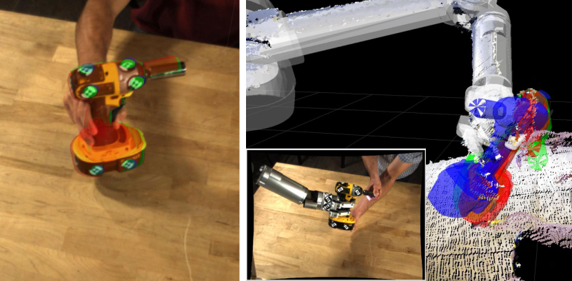
We compare the results from our method with a previously implemented baseline method which tracks objects based on a known pattern of fiducials on the object, using the Bumblebee2 stereo camera. This method is based on an EKF which maintains a distribution over the pose of the object. Fiducials are detected in each camera image using a local template-matching approach (see Fig. 6 left).

Figure 7: Scenario (a): 6-DoF trajectories of the object being manipulated by a human hand, as tracked by the proposed method (red) and the baseline fiducial tracking method (green). The fiducial tracking method is susceptible to errors when fiducials are occluded (e.g., from $t$=33 to $t$=37), while our method is more robust to occlusions.

The template for each fiducial depends on the projection of the expected fiducial pose in the camera. The 3-D position of each fiducial is then reconstructed from their 2-D positions in each camera. The full 6-DoF object pose is solved for by minimizing the squared error between the detected fiducial positions and their corresponding positions in the object model. The object pose thus obtained is treated as an observation which updates the pose distribution in the EKF. This EKF uses the same process models as the ones described in Sect. V, depending on whether the object is in the robot hand or not. Finally, we also contrast these visual tracking methods with estimates of the object pose based on the kinematic model of the robot. The position of the hand is computed using the motor encoders. We compute a fixed offset between the hand and the object at the time of grasping, and assume that this offset remains constant for the entire motion.

VII-B Results

Our algorithm was evaluated in three scenarios: (a) object manipulated by a human (Fig. 6 left), (b) object manipulated by the robot with a secure grasp, and (c) object manipulated by the robot (Fig. 6 right), with a human disturbing the pose of the object in the hand. Videos of each of these scenarios may be found in the multimedia attachment or online at http://youtu.be/MBgggaJq1sY.

Figure 8: Scenario (b): 6-DoF trajectories of the object being manipulated by the robot with a secure grasp. The errors in the forward kinematics method (blue) are due to imprecise joint position sensing under load. The proposed approach (red) followed the baseline (green) closely.

Figure 9: Scenario (c): 6-DoF trajectories of the object being manipulated by the robot, while being disturbed by a human. Changes in the pose of the object in the hand cannot be tracked by the forward kinematics method (blue). Our marker-less approach (red) successfully tracked the object and followed the baseline fiducial-based approach (green) closely.

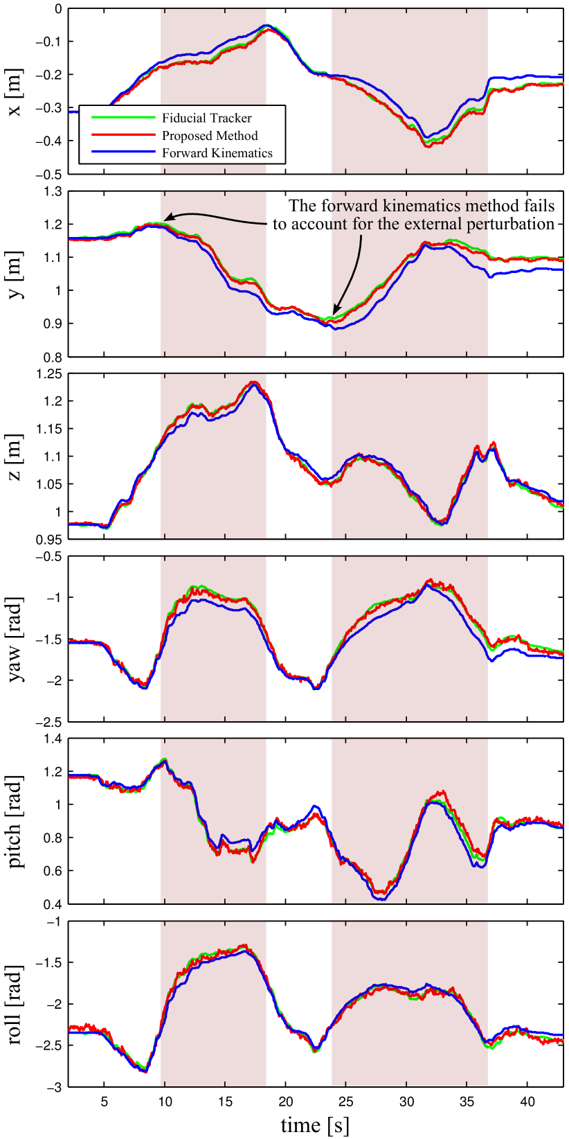
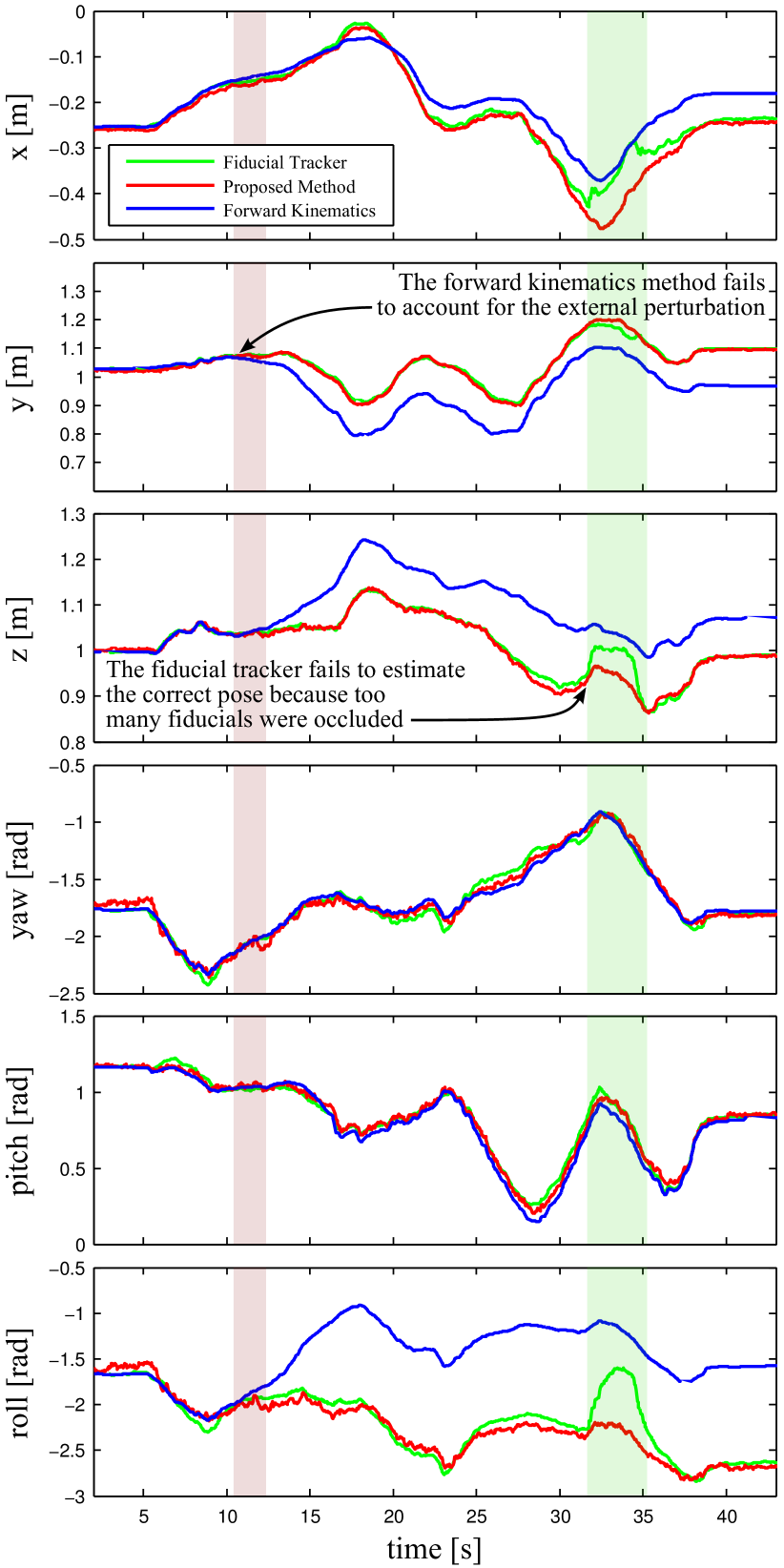
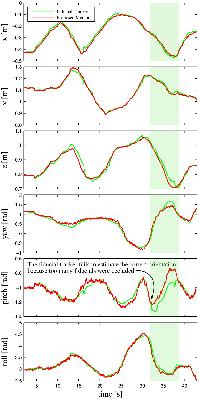
Figure 7 shows the position (x, y, z) and orientation (roll, pitch, yaw) trajectories of the object being moved by a human, as tracked by the baseline fiducial tracking method (shown in green) and our proposed method (shown in red). A qualitative assessment reveals that the fiducial tracking method is susceptible to errors when fiducials are occluded (e.g., from $t$=33 to $t$=37), while the proposed method tracks the object pose more robustly in spite of occlusions.

Results from scenario (b) where the object is manipulated by the robot with a secure grasp are shown in Figure 8. In addition to the baseline method and the proposed method, we also show pose estimates of the object based on the robot kinematic model (in blue). This estimate significantly deviates from the two visual tracking methods due to undetected stretching of the Barrett WAM cables, which is exacerbated by the weight of the object in the hand. Additionally, we introduced external disturbances that did not affect the pose of the object with respect to the hand. Such errors in the forward kinematics model render precise manipulation and tool use impossible without visual tracking and control.

Figure 9 shows results from the final scenario, in which the object is manipulated by the robot, while the pose of the object in the hand is being disturbed by a human. By definition, manipulation tasks involve contact of the object in the hand with the external world. These contacts often result in slippage of the object in the hand, and in such cases visual tracking can be tremendously beneficial for successful completion of the task. Similar to the previous scenario, we notice that the two visual tracking methods perform equally well. In contrast, the forward kinematics method shows large errors as it cannot account for movement of the object in the hand (see Fig. 6 right).

VIII CONCLUSION AND FUTURE WORK

We have presented a probabilistic approach to object tracking using a range camera. Occlusions are explicitly modeled in our approach, which adds robustness and removes the need to filter out points belonging to the robot. Our method is fast enough for real-time tracking performance on a single core of a modern computer, and the sampling process trivially lends itself to parallelization.

In future work, we plan to apply this method to tracking the posture of articulated objects such as the robot arm itself to accurately estimate the arm kinematic configuration. We also plan to apply the probabilistic models developed in this work to alternate sensor modalities such as tactile sensors. Finally, we will use the presented object tracking approach to further close perception-action loops as in [14].

References

- Bohg and Kragic [2010] J. Bohg and D. Kragic. Learning grasping points with shape context. Robotics and Autonomous Systems, 58(4):362–377, 2010.
- Bohg et al. [2013] J. Bohg, A. Morales, T. Asfour, and D. Kragic. Data-Driven Grasp Synthesis - A Survey. IEEE Trans. on Robotics, 2013. In submission. PDF at http://www-clmc.usc.edu/Main/JeannetteBohg.
- Choi and Christensen [2010] C. Choi and H. I. Christensen. Real-time 3d model-based tracking using edge and keypoint features for robotic manipulation. In IEEE Intl Conf on Robotics and Automation, 2010.
- Dang and Allen [2012] H. Dang and P. K. Allen. Semantic Grasping: Planning Robotic Grasps Functionally suitable for an Object Manipulation Task. In IEEE/RSJ Intl Conf on Intelligent Robots and Systems, pages 1311–1317, 2012.
- Doucet et al. [2000] A. Doucet, N. de Freitas, K. Murphy, and S. Russell. Rao-blackwellised particle filtering for dynamic bayesian networks, 2000.
- Fallon et al. [2012] M. F. Fallon, H. Johannsson, and J. J. Leonard. Efficient Scene Simulation for Robust Monte Carlo Localization using an RGB-D Camera. In IEEE Intl Conf on Robotics and Automation, 2012.
- Harris and Stennett [1990] C. Harris and C. Stennett. RAPID - A Video Rate Object Tracker. British Machine Vision Conference, pages 73–77, September 1990.
- Hebert et al. [2012] P. Hebert, N. Hudson, J. Ma, T. Howard, T. Fuchs, M. Bajracharya, and J. Burdick. Combined Shape, Appearance and Silhouette for Simultaneous Manipulator and Object Tracking. In IEEE Intl Conf on Robotics and Automation, 2012.
- Hinterstoisser et al. [2012] S. Hinterstoisser, V. Lepetit, S. Ilic, S. Holzer, G. Bradski, K. Konolige, , and N. Navab. Model based training, detection and pose estimation of texture-less 3d objects in heavily cluttered scenes. In Asian Conference on Computer Vision, 2012.
- Khoshelham and Elberink [2012] K. Khoshelham and S. O. Elberink. Accuracy and Resolution of Kinect Depth Data for Indoor Mapping Applications. Sensors, 12(2):1437–1454, 2012.
- Kragic et al. [2001] D. Kragic, A. T. Miller, and P. K. Allen. Real-time tracking meets online grasp planning. In IEEE Intl Conf on Robotics and Automation, 2001.
- Lai et al. [2011] K. Lai, L. Bo, X. Ren, and D. Fox. Sparse distance learning for object recognition combining rgb and depth information. In IEEE International Conference on on Robotics and Automation, 2011.
- Newcombe et al. [2011] R. A. Newcombe, S. Izadi, O. Hilliges, D. Molyneaux, D. Kim, A. J. Davison, P. Kohli, J. Shotton, S. Hodges, and A. Fitzgibbon. KinectFusion: Real-Time Dense Surface Mapping and Tracking. IEEE Intl Symposium on Mixed and Augmented Reality, 2011.
- Pastor et al. [2011] P. Pastor, L. Righetti, M. Kalakrishnan, and S. Schaal. Online movement adaptation based on previous sensor experiences. In IEEE/RSJ Intl Conf on Intelligent Robots and Systems, pages 365–371, 2011.
- Pastor et al. [2013] P. Pastor, M. Kalakrishnan, J. Binney, J. Kelly, L. Righetti, G. Sukhatme, and S. Schaal. Learning Task Error Models for Manipulation. In IEEE Intl Conf on Robotics and Automation, 2013.
- Ren and Reid [2012] C. Y. Ren and I. Reid. A unified energy minimization framework for model fitting in depth. In ECCV ’12 Workshop on Consumer Depth Cameras for Computer Vision, 2012.
- Righetti et al. [submitted] L. Righetti, M. Kalakrishnan, P. Pastor, J. Binney, J. Kelly, R. C. Voorhies, G. Sukhatme, and S. Schaal. An Autonomous Manipulation System based on Force Control and Optimization. Autonomous Robots Journal Special Issue: Autonomous Grasping and Manipulation, submitted.
- Saxena et al. [2008] A. Saxena, J. Driemeyer, and A. Y. Ng. Robotic Grasping of Novel Objects using Vision. The Intl Journal of Robotics Research, 27(2):157–173, 2008.
- Thrun et al. [2006] S. Thrun, W. Burgard, and D. Fox. Probabilistic Robotics. The MIT Press, 2006.
- Ueda [2012] R. Ueda. Tracking 3d objects with point cloud library. pointclouds.org, 2012. http://pointclouds.org/news/2012 /01/17/tracking-3d-objects-with-point-cloud-library.