Real-Time Simulation of Non-Equilibrium Transport of Magnetization
in Large Open Quantum Spin Systems driven by Dissipation

Abstract

Using quantum Monte Carlo, we study the non-equilibrium transport of magnetization in large open strongly correlated quantum spin $\frac{1}{2}$ systems driven by purely dissipative processes that conserve the uniform or staggered magnetization, disregarding unitary Hamiltonian dynamics. We prepare both a low-temperature Heisenberg ferromagnet and an antiferromagnet in two parts of the system that are initially isolated from each other. We then bring the two subsystems in contact and study their real-time dissipative dynamics for different geometries. The flow of the uniform or staggered magnetization from one part of the system to the other is described by a diffusion equation that can be derived analytically.

Simulating the real-time evolution of large strongly correlated quantum systems is notoriously difficult, due to the dimension of the Hilbert space, which grows exponentially with the system size. In this case, Monte Carlo methods are usually not applicable because importance sampling is prevented by severe sign or complex phase problems Tro05 . While in Euclidean time some severe sign problems have been solved using the meron-cluster algorithm Bie95 ; Cha99 or the fermion bag method Cha10 ; Cha12 ; Cha13 , until recently real-time simulations of quantum systems have been limited to small volumes that are accessible to exact diagonalization, or to gapped 1-d systems to which the time-dependent density matrix renormalization group (DMRG) Whi92 ; Sch05 can be applied. Even then, due to the growth of entanglement, only moderate time intervals can be investigated Vid03 ; Whi04 ; Ver04 ; Zwo04 ; Dal04 ; Bar09 ; Piz13 . Dynamical phenomena in non-equilibrium quantum systems have been studied in Cor74 ; Ber02 ; Aar02 ; Ber08 ; Die08 ; Dal09 ; Die10 ; Mue12 ; Sie13 ; DeG13 ; Hor13 ; Chi15 . Recently, we have developed a new Monte Carlo method that allows us to simulate the real-time evolution of large strongly coupled quantum systems in any dimension for an arbitrary amount of time, for specific dynamics driven by purely dissipative processes that are described by a Lindblad equation Ban14 ; Heb15 . In particular, the unitary time-evolution driven by a Hamiltonian, which would give rise to a severe complex phase problem, has been replaced by a dissipative process. Still severe sign problems arise even for the purely dissipative dynamics, but they have been solved analytically by identifying exact cancellations in the corresponding real-time path integral. Purely dissipative processes play an important role in quantum information processing, for example, in order to prepare specific states for quantum computation Rau01 ; Nie01 ; Chi02 ; Ali04 ; Ver09 or entanglement generation Kra11 . The control of quantum systems by measurements has been investigated in Sug05 ; Pec06 . Ultracold atoms in optical lattices or trapped ions provide platforms in which such dynamics can be engineered in quantum simulation experiments Cir12 ; Lew12 ; Blo12 ; Bla12 .

In this paper, our primary goal is not yet to make contact with concrete cold atoms experiments. Instead, we demonstrate that our ability to classically simulate the real-time dynamics of engineered dissipative processes in large open quantum spin systems puts us in a unique position to study transport phenomena far away from equilibrium. Such processes thus provide a bridge between classical and quantum simulations of real-time quantum dynamics. Here we investigate a low-temperature Heisenberg ferromagnet and an antiferromagnet which are initially isolated from each other in two separate parts of the volume. The two parts, which act as large reservoirs of uniform or staggered magnetization, are then put in contact and evolve in time according to a dissipative process which either conserves the uniform or the staggered magnetization. The corresponding conserved quantity then flows from its reservoir into the other half of the system, through an opening whose size we vary. The non-equilibrium diffusive processes are driven by the gradient of the corresponding conserved quantity. They come to an end only when the staggered or uniform magnetization is homogeneously distributed throughout the entire system. Remarkably, certain aspects of the dynamics are described by a classical diffusion equation which can be derived analytically from the underlying dissipative quantum dynamics. Significantly extdending previous work Ban14 ; Heb15 , the current setting allows us to study the diffusion process of the conserved quantity in real-space.

We consider systems of quantum spins $\frac{1}{2}$ on a square lattice, which are dissipatively coupled to their environment. The dynamics is characterized by a set of Lindblad operators Kos72 ; Lin76 ; Kra83 , $L_{o_{k}}$, that obey $(1-\varepsilon\gamma){\mathbbm{1}}+\sum_{k,o_{k}}L_{o_{k}}^{\dagger}L_{o_{k}}={\mathbbm{1}}$, where $\varepsilon$ is a small time-step. The Lindblad operators induce quantum jumps and $\gamma$ determines their probability per unit time. We will analytically derive the relation between the parameter $\gamma$ and the diffusion coefficient of the classical diffusion equation. The time-evolution of the density matrix is then determined by the Lindblad equation

$$\partial_{t}\rho=\frac{1}{\varepsilon}\sum_{k,o_{k}}\left(L_{o_{k}}\rho L_{o_{k}}^{\dagger}-\frac{1}{2}L_{o_{k}}^{\dagger}L_{o_{k}}\rho-\frac{1}{2}\rho L_{o_{k}}^{\dagger}L_{o_{k}}\right)\,.$$ (1)

We will consider two different dissipative processes whose jump operators $L_{o_{k}}=\sqrt{\varepsilon\gamma}P_{o_{k}}$ are determined by operators $P_{o_{k}}$ that project on the eigenstates of an observable $O$ with eigenvalue $o_{k}$. For the first process (process 1), which conserves the uniform magnetization vector, the observable is the total spin $O^{(1)}=(\vec{S}_{x}+\vec{S}_{y})^{2}$ of a pair of spins $\vec{S}_{x}$ and $\vec{S}_{y}$ located on neighboring lattice sites $x$ and $y$. The projection operators corresponding to total spin 1 or 0 are then given by

$$P_{1}=\left(\begin{array}[]{cccc}1&0&0&0\\ 0&\frac{1}{2}&\frac{1}{2}&0\\ 0&\frac{1}{2}&\frac{1}{2}&0\\ 0&0&0&1\end{array}\right),\quad P_{0}=\left(\begin{array}[]{cccc}0&0&0&0\\ 0&\frac{1}{2}&-\frac{1}{2}&0\\ 0&-\frac{1}{2}&\frac{1}{2}&0\\ 0&0&0&0\end{array}\right).$$ (2)

As we have shown in Ban14 ; Heb15 , the conservation of the total spin in this dissipative process implies that the low-momentum modes of the magnetization equilibrate very slowly. The second dissipative process (process 2), which conserves the 3-component of the staggered magnetization, is characterized by the observable $O^{(2)}=S_{x}^{+}S_{y}^{+}+S_{x}^{-}S_{y}^{-}$ with the three projection operators

$$P_{+}=\left(\begin{array}[]{cccc}\frac{1}{2}&0&0&\frac{1}{2}\\ 0&0&0&0\\ 0&0&0&0\\ \frac{1}{2}&0&0&\frac{1}{2}\end{array}\right),\quad P_{0}=\left(\begin{array}[]{cccc}0&0&0&0\\ 0&1&0&0\\ 0&0&1&0\\ 0&0&0&0\end{array}\right),$$ (11)

$$P_{-}=\left(\begin{array}[]{cccc}\frac{1}{2}&0&0&-\frac{1}{2}\\ 0&0&0&0\\ 0&0&0&0\\ -\frac{1}{2}&0&0&\frac{1}{2}\end{array}\right).$$ (16)

In this case, as we showed in Heb15 , the high-momentum modes of the magnetization (namely those with momenta near the conserved $(\pi,\pi$)-mode representing the staggered magnetization) equilibrate very slowly. Both dissipative processes ultimately converge to a trivial infinite-temperature density matrix that is proportional to the unit-matrix, at least within the sector defined by the value of the corresponding conserved quantity.

As discussed in detail in Ban14 ; Heb15 , the Lindblad equation can be represented by a path integral consisting of a Euclidean time contour that defines an initial density matrix in thermal equilibrium and a real-time Schwinger-Keldysh contour Sch61 ; Kel65 that leads from an initial time $t_{0}$ to a final time $t_{f}$ and back. Remarkably, the probability to reach a specific final state $|f\rangle$ can be computed very efficiently with a loop-cluster algorithm, similar to the one used in Euclidean time Eve93 ; Wie94 ; Bea96 . The cluster rules have been discussed in detail in Heb15 .

We consider a spin $\frac{1}{2}$ Heisenberg model with Hamiltonian $H\!=\!J\sum_{\langle xy\rangle}\!\vec{S}_{x}\cdot\vec{S}_{y}$. In order to prepare an initial density matrix we consider an $L\times 2L$ lattice that is divided into two subsystems of size $L\times L$ each with individual periodic boundary conditions. One system is antiferromagnetic (with $J\!>\!0$) and the other is ferromagnetic and has the opposite exchange coupling. Both subsystems are initialized at the same temperature. The initial density matrix is then subjected to one of the two dissipative real-time processes. During the real-time process the two subsystems are put in contact through two openings of size $L^{\prime}\leq L$ on opposite sides of both systems. This is achieved by changing the original boundary conditions with period $L$ on two sets of $L^{\prime}$ links. These links connect the two subsystems, so that the total system now has boundary conditions with period $2L$ in a strip of transverse size $L^{\prime}$ and the original pair of boundary conditions with period $L$ on the remaining strip of transverse size $L-L^{\prime}$. The transverse direction of size $L$ always has ordinary periodic boundary conditions. Using the loop-cluster algorithm we calculate the expectation value of the 3-component for each spin $S_{x}^{3}$ at the time $t_{f}$ when the 3-components of all spins are finally being measured. The data are separately analyzed for each total value of the conserved uniform or staggered magnetization. By using an improved estimator similar to the one constructed in Ger09 ; Ger11 , we increase the statistics by a factor that grows exponentially with the number of loop-clusters. This improves the accuracy of the numerical data very substantially and leads to the results depicted in Fig. 1 (uniform magnetization) and Fig. 2 (staggered magnetization). As we have discussed in detail in Ban14 ; Heb15 , the dissipative processes give rise to different time scales. While process 1 quickly destroys the initial antiferromagnetic order over a time scale $1/\gamma$, the conserved uniform magnetization undergoes a much slower diffusion process. In particular, in process 1 the magnetization modes with low momentum $p$ equilibrate only over time scales $1/(\gamma a^{2}p^{2})$, where $a$ is the lattice spacing. Similarly, in process 2, which conserves the staggered magnetization, the modes with momenta near $(\pi,\pi)$ are severely slowed down. The dissipative dynamics can be characterized as a heating process that affects different modes at different time scales.

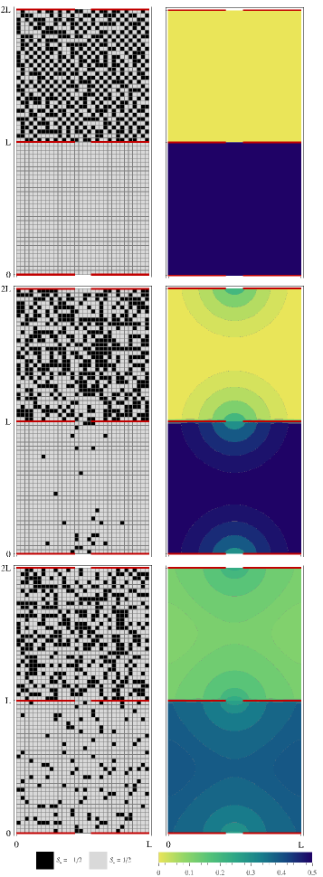
Figure 1: [Color online] Real-time evolution of the uniform magnetization on a $32\times 64$ lattice with an opening of size $L^{\prime}=4a$ for a total uniform magnetization value $M_{u}=\frac{1}{2}(L/a)^{2}=512$ at initial temperature $\beta J=80$. Typical configurations (left) and expectation values of the uniform magnetization (right) at time $t=0$ (top), $50/\gamma$ (middle), and $500/\gamma$ (bottom).

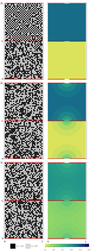
Figure 2: [Color online] Real-time evolution of the staggered magnetization on a $32\times 64$ lattice with an opening of size $L^{\prime}=4a$ for a total staggered magnetization value $M_{s}=\frac{3}{8}(L/a)^{2}=384$ at initial temperature $\beta J=80$. Typical configurations (left) and expectation values of the staggered magnetization (right) at time $t=0$ (top), $50/\gamma$ (middle), and $500/\gamma$ (bottom).

While the underlying diffusive processes are quantum mechanical, the resulting expectation values of the conserved uniform or staggered magnetization are described by a classical diffusion equation

$$\partial_{t}\rho_{x}(t)=\frac{\gamma}{2}\sum_{i}\left[\rho_{x+a\hat{i}}(t)-2\rho_{x}(t)+\rho_{x-a\hat{i}}(t)\right]\,.$$ (17)

Here $\rho_{x}(t)$ is the expectation value of the conserved quantity at the lattice site $x$ at time $t$ and $\hat{i}$ is the unit-vector in the $i$-direction. Interestingly, the classical diffusion equation can be derived analytically from the underlying quantum spin dynamics, and the diffusion coefficient is determined by the parameter $\gamma$ that drives the Lindblad process of eq. (1). The lattice diffusion equation (17) results from the continuity equation

$$\partial_{t}\rho_{x}(t)+\frac{1}{a}\sum_{i}\left[j_{x,i}(t)-j_{x-a\hat{i},i}(t)\right]=0\,,\vspace{-0.1cm}$$ (18)

combined with the lattice gradient equation

$$j_{x,i}(t)=-\frac{a\gamma}{2}\left[\rho_{x+a\hat{i}}(t)-\rho_{x}(t)\right]\,.\vspace{-0.1cm}$$ (19)

Here $j_{x,i}(t)$ is the conserved (uniform or staggered) magnetization current density that flows from the lattice site $x$ to the neighboring lattice site $x+a\hat{i}$ at the time $t$. The continuity equation (18) and the gradient equation (19) can be derived from the underlying real-time path integral that was discussed in detail in Ban14 ; Heb15 . The corresponding spin configurations together with the resulting values for $\rho_{x}(t)$ and $j_{x,i}(t)$ are illustrated in Fig. 3 for the two dissipative processes.

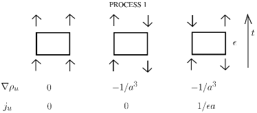
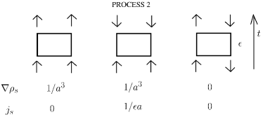
Figure 3: Configurations of two neighboring spins evolving in time, together with the resulting values for $\rho_{x}(t)$ and $j_{x,i}(t)$ for the dissipative process 1 and 2, that conserves the uniform and staggered magnetization, respectively. The current is driven by the gradient of the corresponding density.

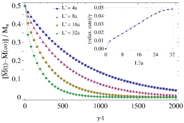
Figure 4: [Color online] Real-time evolution of the total uniform magnetization in the first subsystem $\overline{M}$ for different values of $L^{\prime}$ ($L=32a$, total uniform magnetization $M_{u}=\frac{1}{2}(L/a)^{2}=512$). Inset: Late-time relaxation rate as a function of $L^{\prime}$.

We have also investigated the time-dependence of the total uniform magnetization in the first subsystem (initially ferromagnetic) as a function of the opening size $L^{\prime}$ in dissipative process 1 (cf. Fig. 4). The final state, for which the magnetization is homogeneously distributed throughout the entire system, is reached exponentially at long times. The relaxation rate then depends linearly on the opening size $L^{\prime}$ over a wide range of values of $L^{\prime}$.

For the largest possible size of openings, $L^{\prime}=L$, the diffusion equation reduces to a 1-d problem which can even be solved analytically. The resulting profile of the magnetization density, illustrated in Fig. 5, is given by

$$\rho_{x}(t) = \frac{\rho_{0}}{2}\sum_{\begin{subarray}{c}n=1\\ (n\,\text{odd})\end{subarray}}^{2L/a-1}\frac{a\sin\left(\frac{\pi n}{2L}\left(2x+a\right)\right)}{L\sin\left(\frac{\pi na}{2L}\right)}$$ (20)

$$\times \exp\left(-2\gamma\sin^{2}\left(\frac{\pi na}{2L}\right)t\right)+\frac{\rho_{0}}{2}\,.$$

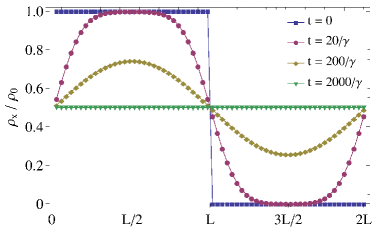
Figure 5: [Color online] The $1$-d profile of the uniform magnetization density ($L^{\prime}=L=32a$) evolves from a step function at the initial time to a uniform distribution at late times.

Certain features of the dissipative processes discussed here resemble classical physics. For example, if finally all spins are projected along the 3-axis at the end of the real-time evolution, the spin configurations on the two branches of the Keldysh contour become identical Ban14 ; Heb15 and their evolution reduces to a Kawasaki dynamics Kaw66 (cf. Fig. 3), which can be captured by a classical diffusion equation. Other aspects of the same dynamics, including the time-evolution of entanglement, do not have this feature, thus underscoring the quantum nature of the corresponding real-time processes. In particular, while the expectation value of the conserved quantity obeys a classical diffusion equation, its probability distribution can only be calculated quantum mechanically. We emphasize that the presented method is not restricted to probing only diagonal elements of the density matrix. Most notably, two-point correlation functions reflecting off-diagonal entries of the density matrix could also be measured very efficiently via improved estimators Bro98 .

It would be most interesting to investigate the non-dissipative pure Hamiltonian dynamics of large closed quantum systems. Due to very severe complex phase problems this is most likely impossible on a classical computer. On the other hand, quantum simulators, for example, using ultracold atoms in optical lattices, are ideally suited for such investigations. It is conceivable to experimentally design a dissipative environment which acts as a projector on singlet and triplet states (process 1) with current technology Tro10 , whereas the realization of process 2 is probably more involved. On the other hand, as we have shown, engineered purely dissipative processes are accessible to very efficient real-time simulation of large open quantum systems using classical computers. Such real-time processes thus provide a bridge between classical and quantum simulation. It will be most interesting to explore other processes, including a weakly coupled Hamiltonian or non-Hermitean Lindblad operators, in order to explore the territory connecting classical and quantum simulation of quantum dynamics in real time.

- (1) M. Troyer and U.-J. Wiese, Phys. Rev. Lett. 94 (2005) 170201.
- (2) W. Bietenholz, A. Pochinsky, and U.-J. Wiese, Phys. Rev. Lett. 75 (1995) 4524.
- (3) S. Chandrasekharan and U.-J. Wiese, Phys. Rev. Lett. 83 (1999) 3116.
- (4) S. Chandrasekharan, Phys. Rev. D82 (2010) 025007.
- (5) S. Chandrasekharan and A. Li, Phys. Rev. Lett. 108 (2012) 140404.
- (6) E. F. Huffman and S. Chandrasekharan, Phys. Rev. B89 (2014) 111101.
- (7) S. R. White, Phys. Rev. Lett. 69 (1992) 2863.
- (8) U. Schollwöck, Rev. Mod. Phys. 77 (2005) 259.
- (9) G. Vidal, Phys. Rev. Lett. 91 (2003) 147902.
- (10) S. R. White and A. E. Feiguin, Phys. Rev. Lett. 93 (2004) 076401.
- (11) F. Verstraete, J. J. Garcia-Ripoll, and J. I. Cirac, Phys. Rev. Lett. 93 (2004) 207204.
- (12) M. Zwolak and G. Vidal, Phys. Rev. Lett. 93 (2004) 207205.
- (13) A. J. Daley, C. Kollath, U. Schollwöck, and G. Vidal, J. Stat. Mech.: Theor. Exp. P04005 (2004).
- (14) T. Barthel, U. Schollwöck, and S. R. White, Phys. Rev. B79 (2009) 245101.
- (15) I. Pizorn, V. Eisler, S. Andergassen, and M. Troyer, New J. Phys. 16 (2014) 073007.
- (16) J. M. Cornwall, R. Jackiw, and E. Tomboulis, Phys. Rev. D10 (1974) 2428.
- (17) J. Berges, Nucl. Phys. A699 (2002) 847.
- (18) G. Aarts, D. Ahrensmeier, R. Baier, J. Berges, and J. Serreau, Phys. Rev. D66 (2002) 045008.
- (19) J. Berges, A. Rothkopf, and J. Schmidt, Phys. Rev. Lett. 101 (2008) 041603.
- (20) S. Diehl, A. Micheli, A. Kantian, B. Kraus, H. P. Büchler, and P. Zoller, Nature Phys. 4 (2008) 878.
- (21) E. G. Dalla Torre, E. Demler, T. Giamarchi, and E. Altman, Nature Phys. 6 (2009) 806.
- (22) S. Diehl, A. Tomadin, A. Micheli, R. Fazio, and P. Zoller, Phys. Rev. Lett. 105 (2010) 015702.
- (23) M. Müller, S. Diehl, G. Pupillo, and P. Zoller, Adv. Atom. Mol. Opt. Phys. 61 (2012) 1.
- (24) L. M. Sieberer, S. D. Huber, E. Altman, and S. Diehl, Phys. Rev. Lett. 110 (2013) 195301.
- (25) C. De Grandi, A. Polkovnikov, and A. W. Sandvik, J. Phys.: Cond. Matt. 25 (2013) 404216.
- (26) B. Horstmann, J. I. Cirac, and G. Giedke, Phys. Rev. A87 (2013) 012108.
- (27) C.-C. Chien, S. Peotta, and M. Di Ventra, arXiv:1504.02907.
- (28) D. Banerjee, F.-J. Jiang, M. Kon, and U.-J. Wiese, Phys. Rev. B90 (2014) 241104.
- (29) F. Hebenstreit, D. Banerjee, M. Hornung, F.-J. Jiang, F. Schranz, and U.-J. Wiese, Phys. Rev. B92 (2015) 035116.
- (30) R. Raussendorf and H. J. Briegel, Phys. Rev. Lett. 86 (2001) 5188.
- (31) M. A. Nielsen, Phys. Lett. A308 (2003) 96.
- (32) A. M. Childs, D. Deotto, E. Farhi, J. Goldstone, S. Gutmann, and A. J. Landahl, Phys. Rev. A66 (2002) 032314.
- (33) P. Aliferis and D. W. Leung, Phys. Rev. A70 (2004) 062314.
- (34) F. Verstraete, M. M. Wolf, and J. I. Cirac, Nature Phys. 5 (2009) 633.
- (35) H. Krauter, C. A. Muschik, K. Jensen, W. Wasilewski, J. M. Petersen, J. I. Cirac, and E. S. Polzik, Phys. Rev. Lett. 107 (2011) 080503.
- (36) M. Sugawara, J. Chem. Phys. 123 (2005) 204115.
- (37) A. Pechen, N. Il’in, F. Shuang, and H. Rabitz, Phys. Rev. A74 (2006) 052102.
- (38) J. I. Cirac and P. Zoller, Nature Phys. 8 (2012) 264.
- (39) M. Lewenstein, A. Sanpera, and V. Ahufinger, “Ultracold Atoms in Optical Lattices: Simulating Quantum Many-Body Systems”, Oxford University Press (2012).
- (40) I. Bloch, J. Dalibard, and S. Nascimbene, Nature Phys. 8 (2012) 267.
- (41) R. Blatt and C. F. Ross, Nature Phys. 8 (2012) 277.
- (42) A. Kossakowski, Rep. Math. Phys. 3 (1972) 247.
- (43) G. Lindblad, Commun. Math. Phys. 48 (1976) 119.
- (44) K. Kraus, States, Effects and Operations, Fundamental Notions of Quantum Theory, Academic, Berlin (1983).
- (45) J. Schwinger, J. Math. Phys. 2 (1961) 407.
- (46) L. V. Keldysh, Sov. Phys. JETP 20 (1965) 1018.
- (47) H. G. Evertz, G. Lana, and M. Marcu, Phys. Rev. Lett. 70 (1993) 875.
- (48) U.-J. Wiese and H.-P. Ying, Z. Phys. B93 (1994) 147.
- (49) B. B. Beard and U.-J. Wiese, Phys. Rev. Lett. 77 (1996) 5130.
- (50) U. Gerber, C. P. Hofmann, F.-J. Jiang, M. Nyfeler, and U.-J. Wiese, J. Stat. Mech.: Theor. Exp. P03021 (2009).
- (51) U. Gerber, C. P. Hofmann, F.-J. Jiang, G. Palma, P. Stebler, and U.-J. Wiese, J. Stat. Mech.: Theor. Exp. P06002 (2011).
- (52) K. Kawasaki, Phys. Rev. 145 (1966) 224.
- (53) R. Brower, S. Chandrasekharan, and U.-J. Wiese, Physica A261 (1998) 520.
- (54) S. Trotzky, Y.-A. Chen, U. Schnorrberger, P. Cheinet, and I. Bloch, Phys. Rev. Lett. 105 (2010) 265303.