Nambu-Goldstone Dark Matter
in a Scale Invariant Bright Hidden Sector

Abstract

We consider a scale invariant extension of the standard model (SM) with a combined breaking of conformal and electroweak symmetry in a strongly interacting hidden $SU(n_{c})$ gauge sector with $n_{f}$ vector-like hidden fermions. The (pseudo) Nambu-Goldstone bosons that arise due to dynamical chiral symmetry breaking are dark matter (DM) candidates. We focus on $n_{f}=n_{c}=3$, where $SU(3)$ is the largest symmetry group of hidden flavor which can be explicitly broken into either $U(1)\times U(1)$ or $SU(2)\times U(1)$. We study DM properties and discuss consistent parameter space for each case. Because of different mechanisms of DM annihilation the consistent parameter space in the case of $SU(2)\times U(1)$ is significantly different from that of $SU(3)$ if the hidden fermions have a SM $U(1)_{Y}$ charge of $O(1)$.

I Introduction

What is the origin of mass? This is a long-standing question and still remains unsolved wilczek .

The recent discovery of the Higgs particle Aad:2012tfa ; Chatrchyan:2012ufa may hint how to go beyond the standard model (SM). The measured Higgs mass and top quark mass Agashe:2014kda are such that the SM remains perturbative below the Planck scale Holthausen:2011aa ; Degrassi:2012ry ; Bezrukov:2012sa . According to Bardeen Bardeen:1995kv , “the SM does not, by itself, have a fine-tuning problem”. Because the Higgs mass term is the only term, which breaks scale invariance at the Lagrangian level in the SM, we may ask about the origin of this mass term. Mostly scale invariance is hardly broken by quantum anomaly Callan:1970yg . Therefore, a dimensional transmutation can occur at the quantum level, which can be used to generate a la Coleman-Weinberg Coleman:1973jx the Higgs mass term in a classically scale invariant extension of the SM Fatelo:1994qf - Kannike:2015apa . Dynamical chiral symmetry breaking Nambu:1960xd ; Nambu:1961tp can also be used Hur:2007uz -Heikinheimo:2014xza . The idea is the same as that of technicolor model Weinberg:1975gm ; Susskind:1978ms , where the only difference is that we now allow the existence of fundamental scalars.

In this paper we consider the latter possibility, in particular the model studied in Hur:2007uz ; Hur:2011sv ; Heikinheimo:2013fta ; Holthausen:2013ota ; Kubo:2014ida . In this model the scale, generated in a QCD-like hidden sector, is transmitted to the SM sector via a real SM singlet scalar $S$ to trigger spontaneous breaking of electroweak (EW) gauge symmetry Hur:2007uz ; Hur:2011sv (see also Kubo:2014ova ). Moreover, due to the dynamical chiral symmetry breaking in the hidden sector there exist Nambu-Goldstone (NG) bosons, which are massive, because the coupling $y$ of $S$ with the hidden sector fermions breaks explicitly chiral symmetry. Therefore, the mass scale of the NG bosons, which are dark matter (DM) candidates, is not independent (as it is not the case in the most of DM models); it is smaller than the hidden sector scale, which is in the TeV region unless the coupling $y$ is very small, i.e. $\mathrel{\mathchoice{\vbox{\offinterlineskip\halign{$\m@th\displaystyle\hfil#\hfil$\cr<\crcr\sim\crcr} }}{\vbox{\offinterlineskip\halign{$\m@th\textstyle\hfil#\hfil$\cr<\crcr\sim\crcr} }}{\vbox{\offinterlineskip\halign{$\m@th\scriptstyle\hfil#\hfil$\cr<\crcr\sim\crcr} }}{\vbox{\offinterlineskip\halign{$\m@th\scriptscriptstyle\hfil#\hfil$\cr<\crcr\sim\crcr} }}}O(10^{-4})$.

As in Holthausen:2013ota ; Kubo:2014ida we employ the Nambu-Jona-Lasinio (NJL) theory Nambu:1960xd ; Nambu:1961tp as an low-energy effective theory of the hidden sector and base our calculations on the self-consistent mean field (SCMF) approximation Hatsuda:1994pi ; Kunihiro:1983ej of the NJL theory, which is briefly outlined in Sect. III. In Holthausen:2013ota ; Kubo:2014ida the maximal global flavor symmetry $SU(3)_{V}$ (along with a $U(1)_{V}$) has been assumed. In this paper we relax this assumption and consider in detail the cases, in which $SU(3)_{V}$ is broken into its subgroups. We find in Sect. IV that the consistent parameter space can be considerably extended if $SU(3)_{V}$ is broken to its subgroup $SU(2)_{V}\times U(1)_{\tilde{B}^{\prime}}$. The main reason is that, if $SU(3)_{V}$ is broken, a new mechanism for the DM annihilation, inverse DM conversion, becomes operative at finite temperature: A pair of lighter DM particles annihilate into a pair of heavier (would-be) DM particles, which subsequently decay into SM particles (mainly into two $\gamma$s).

Before we discuss the DM phenomenology of the model, we develop an effective theory for DM interactions (a linear sigma model) in the framework of the SCMF approximation of the NJL theory. Using the effective theory we compute the DM relic abundance and analyze the direct and indirect DM detection possibilities in Sect. IV. Sect. V is devoted to Conclusion, and in Appendix A we give explicitly the NJL Lagrangian in the SCMF approximation in the case that $SU(3)_{V}$ is broken into $U(1)_{\tilde{B}^{\prime}}\times U(1)_{\tilde{B}}$. In Appendix B the inverse DM (mesons for QCD) propagators and also how the NJL parameters are fixed can be found. The one-loop integrals that are used in our calculations are collected in Appendix C.

II The model

We consider a classically scale invariant extension of the SM studied in Hur:2007uz ; Hur:2011sv ; Heikinheimo:2013fta ; Holthausen:2013ota ; Kubo:2014ida which consists of a hidden $SU(n_{c})_{H}$ gauge sector coupled via a real singlet scalar $S$ to the SM. The hidden sector Lagrangian of the model is written as

$${\cal L}_{\rm H} =-\frac{1}{2}\mbox{Tr}\leavevmode\nobreak\ F^{2}+\mbox{Tr}\leavevmode\nobreak\ \bar{\psi}(i\gamma^{\mu}\partial_{\mu}+g_{H}\gamma^{\mu}G_{\mu}+g^{\prime}Q\gamma^{\mu}B_{\mu}-yS)\psi\leavevmode\nobreak\ ,$$ (1)

where $G_{\mu}$ is the gauge field for the hidden QCD, $B_{\mu}$ is the $U(1)_{Y}$ gauge field, i.e.

$$B_{\mu} = \cos\theta_{W}A_{\mu}-\sin\theta_{W}Z_{\mu}\leavevmode\nobreak\ ,\leavevmode\nobreak\ g^{\prime}=e/\cos\theta_{W}\leavevmode\nobreak\ ,$$ (2)

and the $n_{f}$ (Dirac) fermions $\psi_{i}\leavevmode\nobreak\ (i=1,\dots,n_{f})$ in the hidden sector belong to the fundamental representation of $SU(n_{c})_{H}$. The trace in (1) is taken over the flavor as well as the color indices. The hidden fermions carry a common $U(1)_{Y}$ charge $Q$, implying that they contribute only to $\Pi_{YY}$ of the gauge boson self-energy diagrams so that the $S,T,U$ parameters remain unchanged. The ${\cal L}_{\mathrm{SM}+S}$ part of the total Lagrangian ${\cal L}_{T}={\cal L}_{\rm H}+{\cal L}_{\mathrm{SM}+S}$ contains the SM gauge and Yukawa interactions along with the scalar potential

$$V_{\mathrm{SM}+S} = \lambda_{H}(H^{\dagger}H)^{2}+\frac{1}{4}\lambda_{S}S^{4}-\frac{1}{2}\lambda_{HS}S^{2}(H^{\dagger}H)\leavevmode\nobreak\ ,$$ (3)

where $H^{T}=(H^{+}\leavevmode\nobreak\ ,\leavevmode\nobreak\ (h+iG)\sqrt{2})$ is the SM Higgs doublet field, with $H^{+}$ and $G$ as the would-be Nambu-Goldstone fields . The basic mechanism to trigger the EW symmetry breaking is very simple: The non-perturbative effect of dynamical chiral symmetry breaking in the hidden sector generates a robust scale which is transferred into the SM sector through the real singlet $S$. Then the mass term for the Higgs potential is generated via the Higgs portal term in (3), where the “$-$” in front of the positive $\lambda_{HS}$ is an assumption.

II.1 Global Symmetries

The Yukawa coupling of the hidden fermions with the singlet $S$ breaks explicitly chiral symmetry. Therefore, in the limit of the vanishing Yukawa coupling matrix $y_{ij}$ the global symmetry $SU(n_{f})_{L}\times SU(n_{f})_{R}\times U(1)_{V}\times U(1)_{A}$ is present at the classical level, where $U(1)_{A}$ is broken by anomaly at the quantum level down to its discrete subgroup $Z_{2n_{f}}$, and the unbroken $U(1)_{V}$ ensures the conservation of the hidden baryon number. The non-abelian part of the chiral symmetry $SU(n_{f})_{L}\times SU(n_{f})_{R}$ is broken dynamically down to its diagonal subgroup $SU(n_{f})_{V}$ by the non-vanishing chiral condensates $\langle\bar{\psi}_{i}\psi_{i}\rangle$, implying the existence of $n_{f}^{2}-1$ NG bosons $\phi_{a}\leavevmode\nobreak\ (a=1,\dots,n_{f}^{2}-1)$. In the $n_{f}=3$ case the NG bosons are like the mesons in the real hadron world:

$$\tilde{\pi}^{0} = \phi_{3}\leavevmode\nobreak\ ,\leavevmode\nobreak\ \tilde{\pi}^{\pm}=(\phi_{1}\mp i\phi_{2})/\sqrt{2}\leavevmode\nobreak\ ,\leavevmode\nobreak\$$

$$\tilde{K}^{\pm} = (\phi_{4}\mp i\phi_{5})/\sqrt{2}\leavevmode\nobreak\ ,\leavevmode\nobreak\ \tilde{K}^{0}(\bar{\tilde{K}}^{0})=(\phi_{6}+(-)i\phi_{7})/\sqrt{2}\leavevmode\nobreak\ ,\leavevmode\nobreak\ \tilde{\eta}^{8}=\phi_{8}\leavevmode\nobreak\ ,$$ (4)

where $\tilde{\eta}^{8}$ will mix with $\tilde{\eta}^{0}$ to form the mass eigenstates $\tilde{\eta}$ and $\tilde{\eta}^{\prime}$. (The $\tilde{}$ should avoid the confusion with the real mesons $\pi^{0}$ etc.)

In the presence of the Yukawa coupling the chiral symmetry is explicitly broken; this is the only coupling which breaks the chiral symmetry explicitly. Because of this coupling the NG bosons become massive. An appropriate chiral rotation of $\psi_{i}$ can diagonalize the Yukawa coupling matrix:

$$y_{ij}=y_{i}\delta_{ij}\leavevmode\nobreak\ (y_{i}\geq 0)$$ (5)

can be assumed without loss of generality, which implies that $U(1)^{n_{f}-1}$ corresponding to the elements of the Cartan subalgebra of $SU(n_{f})$ are unbroken. We assume that none of $y_{i}$ vanishes so that all the NG bosons are massive. If two $y_{i}$s are the same, say $y_{1}=y_{2}$, one $U(1)$ is promoted to an $SU(2)$. Similarly, if three $y_{i}$s are the same, a product group $U(1)\times U(1)$ is promoted to an $SU(3)$, and so on. In addition to these symmetry groups, there exists a discrete $Z_{4}$,

$$Z_{4} : \psi_{i}\to\left(\exp i(\pi/2)\gamma_{5}\right)\psi_{i}=i\gamma_{5}\psi_{i}\leavevmode\nobreak\ \mbox{and}\leavevmode\nobreak\ S\to-S\leavevmode\nobreak\ .$$ (6)

This discrete symmetry is anomalous for odd $n_{f}$, because the chiral transformation in (6) is an element of the anomalous $U(1)_{A}$. If $n_{f}$ is even, then the chiral transformation is an element of the anomaly-free subgroup $Z_{2n_{f}}$ of $U(1)_{A}$. Needless to say that this $Z_{4}$ is broken by a non-vanishing vacuum expectation value (VEV) of $S$, which is essential to trigger the EW gauge symmetry breaking.

II.2 Dark Matter Candidates

The NG bosons, which arise due to the dynamical chiral symmetry breaking in the hidden sector, are good DM candidates, because they are neutral and their interactions with the SM part start to exist at the one-loop level so that they are weak. However, not all NG bosons can be DM, because their stability depends on the global symmetries that are in tact. In the following we consider the case for $n_{f}=3$, which can be simply extended to an arbitrary $n_{f}$. For $n_{f}=3$ there are three possibilities of the global symmetries:

$$\mbox{(i)}\leavevmode\nobreak\ U(1)_{\tilde{B}^{\prime}}\times U(1)_{\tilde{B}}\leavevmode\nobreak\ \mbox{if}\leavevmode\nobreak\ y_{1}\neq y_{2}\neq y_{3}\leavevmode\nobreak\ ,$$ (7)

$$\mbox{(ii)}\leavevmode\nobreak\ SU(2)_{V}\times U(1)_{\tilde{B}}\leavevmode\nobreak\ \mbox{if}\leavevmode\nobreak\ y_{1}=y_{2}\neq y_{3}\leavevmode\nobreak\ ,$$ (8)

$$\mbox{(iii)}\leavevmode\nobreak\ SU(3)_{V}\leavevmode\nobreak\ \mbox{if}\leavevmode\nobreak\ y_{1}=y_{2}=y_{3}\leavevmode\nobreak\ ,$$ (9)

where we have suppressed $U(1)_{V}$ which always exists, and the case (iii) has been treated in detail in Kubo:2014ida . Without loss of generality we can assume that the elements of the Cartan subalgebra corresponding to $U(1)_{\tilde{B}^{\prime}}$ and $U(1)_{\tilde{B}}$ are

$${\tilde{B}^{\prime}} = \left(\begin{array}[]{ccc}1&0&0\\ 0&-1&0\\ 0&0&0\\ \end{array}\right)\leavevmode\nobreak\ ,\leavevmode\nobreak\ {\tilde{B}}=\left(\begin{array}[]{ccc}1&0&0\\ 0&1&0\\ 0&0&-2\\ \end{array}\right)\leavevmode\nobreak\ .$$ (16)

In Table I we show the NG bosons for $n_{f}=3$ with their quantum numbers. As we can see from Table I the NG bosons $\tilde{\pi}^{0}$ and $\tilde{\eta}^{8}$ are unstable for the case (i) and in fact can decay into two $\gamma$s, while for the case (ii) only $\tilde{\eta}^{8}$ is unstable. Whether the stable NG bosons can be realistic DM particles is a dynamical question, which we will address later on.

Table 1: The NG bosons and DM candidates for $n_{f}=3$.

	$\tilde{\pi}^{0}$	$\tilde{\pi}^{+}$	$\tilde{\pi}^{-}$		$\tilde{K}^{0}$		$\tilde{K}^{+}$		$\tilde{K}^{-}$		$\tilde{\bar{K}}^{0}$		$\tilde{\eta}^{8}$
$U(1)_{Y}$ charge	$0$	$0$	$0$		$0$		$0$		$0$		$0$		$0$
${\tilde{B}^{\prime}}$	$0$	$2$	$-2$		$-1$		$1$		$-1$		$1$		$0$
${\tilde{B}}$	$0$	$0$	$0$		$3$		$3$		$-3$		$-3$		$0$
$SU(2)_{V}$		${\bf 3}$				${\bf 2}$				${\bf 2}$			${\bf 1}$
$SU(3)_{V}$							${\bf 8}$

II.3 Perturbativity and stability of the scalar potential at high energy

Before we discuss the non-perturbative effects, we consider briefly the perturbative part at high energies, i.e. above the scale of the dynamical chiral symmetry breaking in the hidden sector. As explained in the Introduction, it is essential for our scenario of explaining the origin of the EW scale to work that the scaler potential is unbounded below and the theory remains perturbative (no Landau pole) below the Planck scale. So, we require:

$$\leavevmode\nobreak\ 4\pi>\lambda_{H},\lambda_{S}>0,\leavevmode\nobreak\ 4\pi>\lambda_{HS}>0\leavevmode\nobreak\ ,|y|^{2}<4\pi,$$ (17)

$$\leavevmode\nobreak\ 2\sqrt{\lambda_{H}\lambda_{S}}-\lambda_{HS}>0\leavevmode\nobreak\ .$$ (18)

In the following discussion we assume that the perturbative regime (of the hidden sector) starts around $q_{0}=1$ TeV and $g_{H}^{2}(q_{0})/4\pi\simeq 1$. Although in this model the Higgs mass depends mainly on two parameters, $\lambda_{H}$ and $\lambda_{HS}$, lowering $\lambda_{H}(q_{0})<0.13$ will destabilize the Higgs potential while increasing $\lambda_{H}(q_{0})>0.14$ will require a larger mixing with $S$, which is strongly constrained. Therefore, we consider the RG running of the couplings with $\lambda_{H}(q_{0})$ fixed at $0.135$ and rely on one-loop approximations. In the case that the hypercharge $Q$ of the hidden fermions is different from zero, these fermions contribute to the renormalization group (RG) running of the $U(1)_{Y}$ gauge coupling considerably. We found that $Q\mathrel{\mathchoice{\vbox{\offinterlineskip\halign{$\m@th\displaystyle\hfil#\hfil$\cr<\crcr\sim\crcr} }}{\vbox{\offinterlineskip\halign{$\m@th\textstyle\hfil#\hfil$\cr<\crcr\sim\crcr} }}{\vbox{\offinterlineskip\halign{$\m@th\scriptstyle\hfil#\hfil$\cr<\crcr\sim\crcr} }}{\vbox{\offinterlineskip\halign{$\m@th\scriptscriptstyle\hfil#\hfil$\cr<\crcr\sim\crcr} }}}0.8$ should be satisfied for $g^{\prime}$ to remain perturbative below the Planck scale.

Because of (18) the range of $\lambda_{S}$ is constrained for a given $\lambda_{HS}$ and $\lambda_{H}$: The larger $\lambda_{HS}$ is, the larger $\lambda_{S}$ has to be. But there is an upper limit for $\lambda_{S}(q_{0})$ because of perturbativity . In Fig. 1 we show the allowed area in the $\lambda_{S}-y$ plane for different values of $\lambda_{HS}(q_{0})$ with $\lambda_{H}(q_{0})$ fixed at $0.135$ in the $SU(3)_{V}$ case (9), i.e. $y=y_{1}=y_{2}=y_{3}$ .

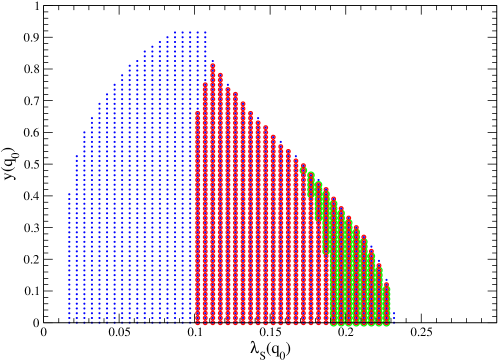
Figure 1: Stability constraint. The allowed area in the $\lambda_{S}-y$ plane for different values of $\lambda_{HS}(q_{0})$ with $\lambda_{H}(q_{0})$ fixed at $0.135$ ($q_{0}=1$ TeV) is shown, where we have used $Q=1/3$ and assumed the $SU(3)_{V}$ flavor symmetry defined in (9). The green circles, red circles and blue points stand for $\lambda_{HS}(q_{0})=0.1,0.06$ and $0.02$.

The green circles, red circles and blue points stand for $\lambda_{HS}(q_{0})=0.1,0.06$ and $0.02$. There will be no allowed region for $\lambda_{HS}(q_{0})\mathrel{\mathchoice{\vbox{\offinterlineskip\halign{$\m@th\displaystyle\hfil#\hfil$\cr>\crcr\sim\crcr} }}{\vbox{\offinterlineskip\halign{$\m@th\textstyle\hfil#\hfil$\cr>\crcr\sim\crcr} }}{\vbox{\offinterlineskip\halign{$\m@th\scriptstyle\hfil#\hfil$\cr>\crcr\sim\crcr} }}{\vbox{\offinterlineskip\halign{$\m@th\scriptscriptstyle\hfil#\hfil$\cr>\crcr\sim\crcr} }}}0.12$. We have used $Q=1/3$, but the allowed area does not depend very much on $Q$ as long as $Q<0.8$ is satisfied (which ensures perturbativity of the $U(1)_{Y}$ gauge coupling). If $SU(3)_{V}$ is broken, then the vertical axis in Fig. 1 represents the largest among $y_{i}$s.

III Nambu-Jona-Lasinio Method

III.1 NJL Lagrangian in a mean-field approximation

Following Holthausen:2013ota we replace the high energy Lagrangian ${\cal L}_{H}$ in (1) by the NJL Lagrangian

$${\cal L}_{\rm NJL} = \mbox{Tr}\leavevmode\nobreak\ \bar{\psi}(i\gamma^{\mu}\partial_{\mu}+g^{\prime}Q\gamma^{\mu}B_{\mu}-yS)\psi+2G\leavevmode\nobreak\ \mbox{Tr}\leavevmode\nobreak\ \Phi^{\dagger}\Phi+G_{D}\leavevmode\nobreak\ (\det\Phi+h.c.)\leavevmode\nobreak\ ,$$ (19)

where

$$\Phi_{ij} = \bar{\psi}_{i}(1-\gamma_{5})\psi_{j}=\frac{1}{2}\sum_{a=0}^{n_{f}^{2}-1}\lambda_{ji}^{a}\mbox{Tr}\leavevmode\nobreak\ \bar{\psi}\lambda^{a}(1-\gamma_{5})\psi\leavevmode\nobreak\ ,$$ (20)

and $\lambda^{a}(a=1,\dots,n_{f}^{2}-1)$ are the Gell-Mann matrices with $\lambda^{0}=\sqrt{2/3}\leavevmode\nobreak\ {\bf 1}$. The effective Lagrangian ${\cal L}_{\rm NJL}$ has three dimensional parameters $G,G_{D}$ and the cutoff $\Lambda$, which have canonical dimensions of $-2$, $-5$ and $1$, respectively. Since the original Lagrangian ${\cal L}_{H}$ has only one independent scale, the parameters $G,G_{D}$ and $\Lambda$ are not independent. We restrict ourselves to $n_{c}=n_{f}=3$, because in this case these parameters, up-to an overall scale, can be approximately fixed from hadron physics Kunihiro:1983ej ; Hatsuda:1994pi . The six-fermi interaction in (19) is present due to chiral anomaly of the axial $U(1)_{A}$ and is invariant under $Z_{6}$, so that the NJL Lagrangian (19) has the same global symmetry as the high energy Lagrangian (1). Furthermore, as we mentioned in Sect. II A, we can assume without loss of generality that the Yukawa coupling matrix $y$ is diagonal (see (5)). To deal with the non-renormalizable Lagrangian (19) we employ Holthausen:2013ota the SCMF approximation which has been intensely studied by Hatsuda and Kunihiro Kunihiro:1983ej ; Hatsuda:1994pi for hadron physics. The NJL parameters for the hidden QCD is then obtained by the upscaling of the actual values of $G,G_{D}$ and the cutoff $\Lambda$ from QCD hadron physics. That is, we assume that the dimensionless combinations

$$G^{1/2}\Lambda = 1.82\leavevmode\nobreak\ ,\leavevmode\nobreak\ (-G_{D})^{1/5}\Lambda=2.29\leavevmode\nobreak\ ,$$ (21)

which are satisfied for hadrons, remain unchanged for a higher scale of $\Lambda$.

Below we briefly outline the SCMF approximation. We go via a Bogoliubov-Valatin transformation from the perturbative vacuum to the “BCS” vacuum, which we simply denote by $|0\rangle$. This vacuum is so defined that the mesons (mean fields) are collected in the VEV of the chiral bilinear:

$$\varphi \equiv \langle 0|\bar{\psi}(1-\gamma_{5})\lambda^{a}\psi|0\rangle=-\frac{1}{4G}\left(\mbox{diag}(\tilde{\sigma}_{1},\tilde{\sigma}_{2},\tilde{\sigma}_{3})+i(\lambda^{a})^{T}\phi_{a}\right)\leavevmode\nobreak\ ,$$ (22)

where we denote the pseudo NG boson fields after spontaneous chiral symmetry breaking by $\phi_{a}$. The dynamics of the hidden sector creates a nonvanishing chiral condensate $\langle 0|\bar{\psi}_{i}\psi_{i}|0\rangle$ which is nothing but $-\langle\tilde{\sigma}_{i}\rangle/4G$. The actual value of $\langle\tilde{\sigma}_{i}\rangle$ can be obtained through the minimization of the scalar potential, as we describe shortly. In the SCMF approximation one splits up the NJL Lagrangian (19) into the sum

$$\mathcal{L}_{\rm NJL} = \mathcal{L}_{0}+\mathcal{L}_{I}\leavevmode\nobreak\ ,$$ (23)

where $\mathcal{L}_{I}$ is normal ordered (i.e. $\langle 0|\mathcal{L}_{I}|0\rangle=0$), and $\mathcal{L}_{0}$ contains at most fermion bilinears which are not normal ordered. At the non-trivial lowest order only ${\cal L}_{0}$ is relevant for the calculation of the effective potential, the DM mass and the DM interactions. The explicit form for $\mathcal{L}_{0}$ can be found in Appendix A. The effective potential can be obtained by integrating out the hidden fermion fields in the BCS vacuum. At the one-loop level we find

$$V_{\rm NJL}(\tilde{\sigma}_{i},S) =\frac{1}{8G}\sum_{i=1,2,3}\tilde{\sigma}_{i}^{2}-\frac{G_{D}}{16G^{3}}\tilde{\sigma}_{1}\tilde{\sigma}_{2}\tilde{\sigma}_{3}-\sum_{i=1,2,3}n_{c}I_{V}(M_{i})\leavevmode\nobreak\ ,$$ (24)

where $I_{V}(m)$ is given in Eq. (102), and the constituent fermion masses $M_{i}$ are given by

$$M_{i} = \tilde{\sigma}_{i}+y_{i}S-\frac{G_{D}}{8G^{2}}\tilde{\sigma}_{i+1}\tilde{\sigma}_{j+2},\leavevmode\nobreak\$$ (25)

where $\tilde{\sigma}_{4}=\tilde{\sigma}_{1}$ and $\tilde{\sigma}_{5}=\tilde{\sigma}_{2}$. Once the free parameters of the model $y_{i},\lambda_{H},\lambda_{HS},\lambda_{S}$ are given, the VEVs of $\tilde{\sigma}_{i}$ and $S$ can be determined through the minimization of the scalar potential $V_{\rm SM+S}+V_{\rm NJL}$, where $V_{\rm SM+S}$ is defined in (3). After the minimum of the scalar potential is fixed, the mass spectrum for the CP-even particles $h,S$ and $\tilde{\sigma}$ as well as the DM candidates with their properties are obtained.

III.2 The value of $y$ and hidden Chiral Phase Transition

The Yukawa coupling in (1) violates explicitly chiral symmetry and plays a similar role as the current quark mass in QCD. It is well known that the nature of chiral phase transition in QCD depends on the value of the current quark mass. Therefore, it is expected that the value of $y$ strongly influences the nature of the chiral phase transition in the hidden sector, which has been confirmed in Holthausen:2013ota . The hidden chiral phase transition occurs above the EW phase transition, where the nature of the EW phase transition is not known yet. In the following discussions, we restrict ourselves to

$$y\mathrel{\mathchoice{\vbox{\offinterlineskip\halign{$\m@th\displaystyle\hfil#\hfil$\cr<\crcr\sim\crcr} }}{\vbox{\offinterlineskip\halign{$\m@th\textstyle\hfil#\hfil$\cr<\crcr\sim\crcr} }}{\vbox{\offinterlineskip\halign{$\m@th\scriptstyle\hfil#\hfil$\cr<\crcr\sim\crcr} }}{\vbox{\offinterlineskip\halign{$\m@th\scriptscriptstyle\hfil#\hfil$\cr<\crcr\sim\crcr} }}}0.006\leavevmode\nobreak\ ,$$ (34)

because in this case the hidden chiral phase transition is a strong first order transition Holthausen:2013ota and can produce gravitational wave back ground Witten:1984rs ; Hogan:1986qda , which could be observed by future experiments such as Evolved Laser Interferometer Space Antenna (eLISA) experiment AmaroSeoane:2012km . Needless to say that the smaller is $y$, the better is the NJL approximation to chiral symmetry breaking.

IV Dark Matter Phenomenology

IV.1 Dark Matter Masses

Our DM candidates are the pseudo NG bosons, which occur due to the dynamical chiral symmetry breaking in the hidden sector. They are CP-odd scalars, and their masses are generated at one-loop in the SCMF approximation as the real meson masses, where we here, too, restrict ourselves to $n_{c}=n_{f}=3$. Therefore, their inverse propagators can be calculated in a similar way as in the QCD case, which is given in Appendix B.

First we consider the $SU(3)_{V}$ case (9) to obtain the DM mass $m_{\rm DM}$ and the mass of the singlet $m_{S}$ for $0.001\mathrel{\mathchoice{\vbox{\offinterlineskip\halign{$\m@th\displaystyle\hfil#\hfil$\cr<\crcr\sim\crcr} }}{\vbox{\offinterlineskip\halign{$\m@th\textstyle\hfil#\hfil$\cr<\crcr\sim\crcr} }}{\vbox{\offinterlineskip\halign{$\m@th\scriptstyle\hfil#\hfil$\cr<\crcr\sim\crcr} }}{\vbox{\offinterlineskip\halign{$\m@th\scriptscriptstyle\hfil#\hfil$\cr<\crcr\sim\crcr} }}}y_{1}=y_{2}=y_{3}\mathrel{\mathchoice{\vbox{\offinterlineskip\halign{$\m@th\displaystyle\hfil#\hfil$\cr<\crcr\sim\crcr} }}{\vbox{\offinterlineskip\halign{$\m@th\textstyle\hfil#\hfil$\cr<\crcr\sim\crcr} }}{\vbox{\offinterlineskip\halign{$\m@th\scriptstyle\hfil#\hfil$\cr<\crcr\sim\crcr} }}{\vbox{\offinterlineskip\halign{$\m@th\scriptscriptstyle\hfil#\hfil$\cr<\crcr\sim\crcr} }}}0.006$. In Fig. 2 (left) we show the area in the $m_{S}$-$m_{\rm DM}$ plane, in which we obtain a correct Higgs mass, while imposing the perturbativity (17) as well as stability (18) constraints. The upper limit of $m_{\rm DM}$ for a given $m_{S}$ is due to the upper limit of the Yukawa coupling (see (34)), while its lower limit comes from the lower limit of the Yukawa coupling, which is taken to be $0.0005$ here. The upper limit for $m_{S}$ is dictated by the upper limit of $\lambda_{S}$, which is fixed by the perturbativity and stability constraints (17) and (18). The lowest value of $m_{S}$, $250$ GeV, comes from the lowest value of $\lambda_{S}$, which is set at $0.05$ here. If $SU(3)_{V}$ is only slightly broken, the DM mass will not change very much.

We next consider the $U(1)_{\tilde{B}^{\prime}}\times U(1)_{\tilde{B}}$ case (7). We may assume without loss of generality that the hierarchy $y_{1}<y_{2}<y_{3}$ is satisfied. In Fig. 2 (right) we show the ratio $m_{\tilde{\pi}^{0}}/m_{\tilde{\pi}^{\pm}}$ versus $y_{1}/y_{2}$, where we have fixed $y_{1}$ and $y_{3}$ at $0.002$ and $0.006$, respectively.

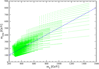
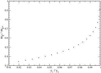
Figure 2: Left: The area in the $m_{S}$-$m_{\rm DM}$ plane for $0.0005<y_{1}=y_{2}=y_{3}<0.006$ in the $SU(3)_{V}$ case (9), where $m_{\rm DM}=m_{\tilde{\pi}^{0}}=m_{\tilde{\pi}^{\pm}}=m_{\tilde{K}^{0}}=m_{\tilde{K}^{\pm}}=m_{\tilde{\eta}}$. The ratio $m_{S}/m_{\rm DM}=2$ is satisfied on the blue dashed line, on which the resonance condition in the s-channel diagram for the DM annihilation (Fig. 10) is satisfied. Right: The ratio $m_{\tilde{\pi}^{0}}/m_{\tilde{\pi}^{\pm}}$ versus $y_{1}/y_{2}$ in the $U(1)_{\tilde{B}^{\prime}}\times U(1)_{\tilde{B}}$ case (7), where $y_{1}$ and $y_{3}$ are fixed at $0.002$ and $0.006$, respectively. The constraints imposed on $\lambda_{H},\lambda_{HS}$ and $\lambda_{S}$ are such that we obtain a correct Higgs mass and the perturbativity (17) as well as stability (18) constraints are satisfied.

We can conclude from Fig. 2 (right) that $\tilde{\pi}^{0}$ is the lightest among the pseudo NG bosons and the ratio $m_{\tilde{\pi}^{0}}/m_{\tilde{\pi}^{\pm}}$ does not practically depend on the scalar couplings $\lambda_{H},\lambda_{HS}$ and $\lambda_{S}$. The $SU(2)_{V}$ case (8) can be realized if two of $y_{i}$ are the same. There are two independent possibilities: (a)  $y_{1}=y_{2}<y_{3}$, and (b)  $y_{1}<y_{2}=y_{3}$. The mass spectrum for the case (b) is similar to that for the $U(1)_{\tilde{B}^{\prime}}\times U(1)_{\tilde{B}}$ case. In particular, $\tilde{\pi}^{0}$ is the lightest among the pseudo NG bosons. As for the case (a) the mass hierarchy

$$m_{\tilde{\pi}} = m_{\tilde{\pi}^{0}}=m_{\tilde{\pi}^{\pm}}<m_{\tilde{K}}=m_{\tilde{K}^{0}}=m_{\tilde{K}^{\pm}}<m_{\tilde{\eta}}$$ (35)

is always satisfied.

The different type of the DM mass spectrum will have an important consequence when discussing the DM relic abundance.

IV.2 Effective interactions for DM Decay and Annihilations

As discussed in Sect. II B, if the $SU(3)_{V}$ flavor symmetry is broken to $U(1)_{\tilde{B^{\prime}}}\times U(1)_{\tilde{B}}$, there will be two real decaying would-be DM particles $\tilde{\eta},\tilde{\pi}^{0}$, and three pairs of complex DM particles $(\tilde{K}^{0},\tilde{\bar{K}}^{0}),\tilde{K}^{\pm}$ and $\tilde{\pi}^{\pm}$. Here we will derive effective interactions for these DM fields by integrating out the hidden fermions at the one-loop order. The one-loop integrals and their lowest order expressions of expansion in the external momenta in the large $\Lambda$ limit are given in Appendix B. Except for the $\phi\mbox{-}\phi\mbox{-}\gamma$ and $\phi\mbox{-}\gamma\mbox{-}\gamma$ interactions, we assume $SU(2)_{V}$ flavor symmetry, i.e.

$$\langle\sigma_{1}\rangle = \langle\sigma_{2}\rangle,\leavevmode\nobreak\ M_{1}=M_{2}\leavevmode\nobreak\ ,Z_{\tilde{K}}=Z_{\tilde{K}^{\pm}}=Z_{\tilde{K}^{0}}\leavevmode\nobreak\ ,\leavevmode\nobreak\ Z_{\tilde{\pi}}=Z_{\tilde{\pi}^{\pm}}=Z_{\tilde{\pi}^{0}}\leavevmode\nobreak\ ,$$ (36)

where $Z$s are the wave function renormalization constants given in (99). This is because, we have to assume at least $SU(2)_{V}$ for a realistic parameter space as we will see.

$\bullet$$\phi\mbox{-}\phi\mbox{-}\gamma$
The corresponding one-loop diagram is shown in Fig. 3, where the right diagram in Fig. 3 yields zero contribution.

$${\cal L}_{\phi^{2}\gamma}=A^{\mu\nu}\left(G_{K^{+}K^{-}\gamma}\partial_{\mu}\tilde{K}^{+}\partial_{\nu}\tilde{K}^{-}+G_{K^{0}\bar{K}^{0}\gamma}\partial_{\mu}\tilde{K}^{0}\partial_{\nu}\tilde{\bar{K}}^{0}+G_{\pi^{+}\pi^{-}\gamma}\partial_{\mu}\tilde{\pi}^{+}\partial_{\nu}\tilde{\pi}^{-}\right)$$

$$+Z^{\mu\nu}\left(G_{K^{+}K^{-}Z}\partial_{\mu}\tilde{K}^{+}\partial_{\nu}\tilde{K}^{-}+G_{K^{0}\bar{K}^{0}Z}\partial_{\mu}\tilde{K}^{0}\partial_{\nu}\tilde{\bar{K}}^{0}+G_{\pi^{+}\pi^{-}Z}\partial_{\mu}\tilde{\pi}^{+}\partial_{\nu}\tilde{\pi}^{-}\right)\leavevmode\nobreak\ ,$$ (37)

where $A(Z)_{\mu\nu}=\partial_{\mu}A(Z)_{\nu}-\partial_{\nu}A(Z)_{\mu}$. The effective couplings in the large $\Lambda$ limit are

$$G_{K^{+}K^{-}\gamma} = 2Z_{\tilde{K}^{\pm}}n_{c}eQ\left(1-\frac{G_{D}}{8G^{2}}\langle\sigma_{2}\rangle\right)^{2}I_{\phi^{2}\gamma}(M_{3},M_{1})\leavevmode\nobreak\ ,$$ (38)

$$G_{K^{0}\bar{K}^{0}\gamma} = 2Z_{\tilde{K}^{0}}n_{c}eQ\left(1-\frac{G_{D}}{8G^{2}}\langle\sigma_{1}\rangle\right)^{2}I_{\phi^{2}\gamma}(M_{3},M_{2})\leavevmode\nobreak\ ,$$

$$G_{\pi^{+}\pi^{-}\gamma} = 2Z_{\tilde{\pi}^{\pm}}n_{c}eQ\left(1-\frac{G_{D}}{8G^{2}}\langle\sigma_{3}\rangle\right)^{2}I_{\phi^{2}\gamma}(M_{2},M_{1})\leavevmode\nobreak\ ,$$

$$G_{K^{+}K^{-}Z} = -t_{W}G_{K^{+}K^{-}\gamma}\leavevmode\nobreak\ ,G_{K^{0}\bar{K}^{0}Z}=-t_{W}G_{K^{0}\bar{K}^{0}\gamma}\leavevmode\nobreak\ ,G_{\pi^{+}\pi^{-}Z}=-t_{W}G_{\pi^{+}\pi^{-}\gamma}\leavevmode\nobreak\ ,$$

$t_{W}^{2}=(\sin\theta_{W}/\cos\theta_{W})^{2}\simeq 0.3$, and $I_{\phi\gamma^{2}}(m_{a},m_{b})$ is given in (105). In the $SU(2)_{V}$ limit, we obtain $G_{K^{0}\bar{K}^{0}\gamma}=G_{K^{+}K^{-}\gamma}$ and $G_{\pi^{+}\pi^{-}\gamma}=0$, because $I_{\phi^{2}\gamma}(m_{a},m_{b})\to(m_{b}-m_{a})/(48\pi^{2}m_{a}^{3})$ as $m_{b}\to m_{a}$.

$\bullet$$\phi\to\gamma\gamma$
The diagram in Fig. 4 shows the decay of $\tilde{\eta},\tilde{\pi}^{0}$ and $S$ into two $\gamma$s, but they can also decay two $Z$s and $\gamma$ and $Z$, if the processes are kinematically allowed. Using the NJL Lagrangian (88) and (106) in Appendix C we find that the effective interaction takes the form

$${\cal L}_{\phi\gamma^{2}}=\frac{1}{4}\tilde{\eta}\epsilon^{\mu\nu\alpha\beta}\left(\frac{1}{2}G_{\eta\gamma^{2}}\leavevmode\nobreak\ A_{\mu\nu}A_{\alpha\beta}+G_{\eta\gamma Z}\leavevmode\nobreak\ A_{\mu\nu}Z_{\alpha\beta}+\frac{1}{2}G_{\eta Z^{2}}\leavevmode\nobreak\ Z_{\mu\nu}Z_{\alpha\beta}\right)$$

$$+\frac{1}{4}\tilde{\pi}^{0}\epsilon^{\mu\nu\alpha\beta}\left(\frac{1}{2}G_{\pi^{0}\gamma^{2}}\leavevmode\nobreak\ A_{\mu\nu}A_{\alpha\beta}+G_{\pi^{0}\gamma Z}\leavevmode\nobreak\ A_{\mu\nu}Z_{\alpha\beta}+\frac{1}{2}G_{\pi^{0}Z^{2}}\leavevmode\nobreak\ Z_{\mu\nu}Z_{\alpha\beta}\right)\leavevmode\nobreak\ ,$$ (39)

where in the large $\Lambda$ limit

$$G_{\eta\gamma^{2}} = Z_{\tilde{\eta}}^{1/2}n_{c}\frac{\alpha}{\sqrt{3}\pi}Q^{2}\left[\left(1-\frac{G_{D}}{8G^{2}}(2\langle\sigma_{2}\rangle-\langle\sigma_{3}\rangle)\right)M_{1}^{-1}\right.$$ (40)

$$\left.+\left(1-\frac{G_{D}}{8G^{2}}(2\langle\sigma_{1}\rangle-\langle\sigma_{3}\rangle)\right)M_{2}^{-1}-\left(2-\frac{G_{D}}{8G^{2}}(2\langle\sigma_{1}\rangle-\langle\sigma_{3}\rangle)\right)M_{3}^{-1}\right],$$

$$G_{\eta\gamma Z} = -t_{W}G_{\eta\gamma^{2}},\leavevmode\nobreak\ G_{\eta Z^{2}}=t_{W}^{2}G_{\eta\gamma^{2}}\leavevmode\nobreak\ ,$$

$$G_{\pi^{0}\gamma^{2}} = Z_{\tilde{\pi}}^{1/2}n_{c}\frac{\alpha}{\pi}Q^{2}\left(1-\frac{G_{D}}{8G^{2}}\langle\sigma_{3}\rangle\right)\left(M_{1}^{-1}-M_{2}^{-1}\right)\leavevmode\nobreak\ ,$$ (41)

$$G_{\pi^{0}\gamma Z} = -t_{W}G_{\pi^{0}\gamma^{2}},\leavevmode\nobreak\ G_{\pi^{0}Z^{2}}=t_{W}^{2}G_{\pi^{0}\gamma^{2}}\leavevmode\nobreak\ .$$

As we see from (41), the $\tilde{\pi}^{0}\to\gamma\gamma$ decay vanishes in the $SU(2)_{V}$ limit, because $M_{1}=M_{2}$ in this limit.

The decay of $S$ into two $\gamma$, two $Z$ and $\gamma Z$ can be described by

$${\cal L}_{S\gamma^{2}}=S\left(\frac{1}{2}G_{S\gamma^{2}}\leavevmode\nobreak\ A_{\mu\nu}A^{\mu\nu}+G_{S\gamma Z}\leavevmode\nobreak\ A_{\mu\nu}Z^{\mu\nu}+\frac{1}{2}G_{SZ^{2}}\leavevmode\nobreak\ Z_{\mu\nu}Z^{\mu\nu}\right)\leavevmode\nobreak\ ,$$ (42)

where we find from (139)

$$G_{S\gamma^{2}} = \frac{\alpha}{3\pi}Q^{2}\sum_{i=1,2,3}y_{i}M_{i}^{-1},$$ (43)

$$G_{S\gamma Z} = -t_{W}G_{S\gamma^{2}},\leavevmode\nobreak\ G_{SZ^{2}}=t_{W}^{2}G_{S\gamma^{2}}\leavevmode\nobreak\ .\leavevmode\nobreak\$$ (44)

$\bullet$Dark matter conversion
The diagrams in Figs. 5 and 6 are examples of DM conversion, in which two incoming DM particles are annihilated into a pair of two DM particles which are different from the incoming ones. There are DM conversion amplitudes, which do not vanish in the $SU(3)_{V}$ limit, and those which vanish in the limit. Except the last $\eta K^{2}\pi$ interaction term, the effective interaction term below do not vanish the $SU(3)_{V}$ limit.

$${\cal L}_{\phi^{4}} = \frac{1}{2}G_{\eta^{2}K^{2}}\leavevmode\nobreak\ \tilde{\eta}^{2}\left(\tilde{K}^{0}\tilde{\bar{K}}^{0}+\tilde{K}^{+}\tilde{K}^{-}\right)+\frac{1}{2}G_{\eta^{2}\pi^{2}}\leavevmode\nobreak\ \tilde{\eta}^{2}\left(\frac{1}{2}(\tilde{\pi}^{0})^{2}+\tilde{\pi}^{+}\tilde{\pi}^{-}\right)$$ (45)

$$+G_{K^{2}\pi^{2}}\left(\tilde{K}^{0}\tilde{\bar{K}}^{0}+\tilde{K}^{+}\tilde{K}^{-}\right)\left(\frac{1}{2}(\tilde{\pi}^{0})^{2}+\tilde{\pi}^{+}\tilde{\pi}^{-}\right)$$

$$+G_{\eta K^{2}\pi}\tilde{\eta}\left((\tilde{K}^{0}\tilde{\bar{K}}^{0}-\tilde{K}^{+}\tilde{K}^{-})\tilde{\pi}^{0}+\sqrt{2}\tilde{K}^{0}\tilde{K}^{-}\tilde{\pi}^{+}+\sqrt{2}\tilde{\bar{K}}^{0}\tilde{K}^{+}\tilde{\pi}^{-}\right)\leavevmode\nobreak\ ,$$

where

$$G_{\eta^{2}K^{2}} = \frac{4}{3}Z_{\tilde{\eta}}Z_{\tilde{K}}n_{c}\left(1-\frac{G_{D}}{8G^{2}}\langle\sigma_{1}\rangle\right)^{2}\left[\left(1-\frac{G_{D}}{8G^{2}}(2\langle\sigma_{1}\rangle-\langle\sigma_{3}\rangle)\right)^{2}\leavevmode\nobreak\ I_{\phi^{4}}^{2A}(M_{1},M_{3})\right.$$ (46)

$$+4\left(1-\frac{G_{D}}{8G^{2}}\langle\sigma_{1}\rangle\right)^{2}\leavevmode\nobreak\ I_{\phi^{4}}^{2A}(M_{3},M_{1})$$

$$\left.-2\left(1-\frac{G_{D}}{8G^{2}}\langle\sigma_{1}\rangle\right)\left(1-\frac{G_{D}}{8G^{2}}(2\langle\sigma_{1}\rangle-\langle\sigma_{3}\rangle)\right)\leavevmode\nobreak\ I_{\phi^{4}}^{1A}(M_{1},M_{3})\right]$$

$$+\frac{4}{3}Z_{\tilde{\eta}}Z_{\tilde{K}}n_{c}\left(\frac{G_{D}}{8G^{2}}\right)^{2}\left(I_{\phi^{4}}^{1B}(M_{1},M_{3})+2I_{\phi^{4}}^{2B}(M_{1})\right)\leavevmode\nobreak\ ,$$

$$G_{\eta^{2}\pi^{2}} = 4Z_{\tilde{\eta}}Z_{\tilde{\pi}}n_{c}\left(1-\frac{G_{D}}{8G^{2}}\langle\sigma_{3}\rangle\right)^{2}\left(1-\frac{G_{D}}{8G^{2}}(2\langle\sigma_{1}\rangle-\langle\sigma_{3}\rangle)\right)^{2}I_{\phi^{4}}^{3A}(M_{1})$$ (47)

$$+\frac{4}{3}Z_{\tilde{\eta}}Z_{\tilde{\pi}}n_{c}\left(\frac{G_{D}}{8G^{2}}\right)^{2}\left(4I_{\phi^{4}}^{2B}(M_{1})-I_{\phi^{4}}^{2B}(M_{3})\right)\leavevmode\nobreak\ ,$$

$$G_{K^{2}\pi^{2}} = 4Z_{\tilde{K}}Z_{\tilde{\pi}}n_{c}\left(1-\frac{G_{D}}{8G^{2}}\langle\sigma_{1}\rangle\right)^{2}\left(1-\frac{G_{D}}{8G^{2}}\langle\sigma_{3}\rangle\right)^{2}I_{\phi^{4}}^{2A}(M_{1},M_{3})$$ (48)

$$+4Z_{\tilde{\pi}}Z_{\tilde{K}}n_{c}\left(\frac{G_{D}}{8G^{2}}\right)^{2}I_{\phi^{4}}^{1B}(M_{1},M_{3})\leavevmode\nobreak\ ,$$

$$G_{\eta K^{2}\pi} = \frac{4}{\sqrt{3}}Z_{\tilde{\eta}}^{1/2}Z_{\tilde{K}}Z_{\tilde{\pi}}^{1/2}n_{c}\left(1-\frac{G_{D}}{8G^{2}}\langle\sigma_{1}\rangle\right)^{2}\left(1-\frac{G_{D}}{8G^{2}}\langle\sigma_{3}\rangle\right)$$ (49)

$$\times\left[\left(1-\frac{G_{D}}{8G^{2}}\langle\sigma_{1}\rangle\right)\leavevmode\nobreak\ I_{\phi^{4}}^{1A}(M_{1},M_{3})-\left(1-\frac{G_{D}}{8G^{2}}(2\langle\sigma_{1}\rangle-\langle\sigma_{3}\rangle)\right)\leavevmode\nobreak\ I_{\phi^{4}}^{2A}(M_{1},M_{3})\right]$$

$$+\frac{4}{\sqrt{3}}Z_{\tilde{\eta}}^{1/2}Z_{\tilde{K}}Z_{\tilde{\pi}}^{1/2}n_{c}\left(\frac{G_{D}}{8G^{2}}\right)^{2}\left(I_{\phi^{4}}^{1B}(M_{1},M_{3})-I_{\phi^{4}}^{2B}(M_{1})\right)\leavevmode\nobreak\ ,$$

and $I_{\phi^{4}}^{1A}(m_{a},m_{b})$ etc. are defined in (109)-(113) in Appendix C. We have not included the contributions from the diagram like one in Fig. 6, because they are negligibly suppressed in a realistic parameter space, in which $SU(3)_{V}$ is only weakly broken. Similarly, $G_{\eta K^{2}\pi}$, too, is negligibly small ($G_{\eta K^{2}\pi}/G_{\eta^{2}K^{2}}\sim 10^{-4}$), so that we will not take into account the $\eta K^{2}\pi$ interactions in computing the DM relic abundance.

$\bullet$Dark matter coupling with $S$
The diagrams in Figs. 7 and 8 show dark matter interactions with the singlet $S$. The DM coupling with $S$ (Fig. 7) can be described by

$${\cal L}_{\phi^{2}S} = S\left(\frac{1}{2}G_{\eta^{2}S}\tilde{\eta}^{2}++G_{K^{2}S}(\tilde{K}^{0}\tilde{\bar{K}}^{0}+\tilde{K}^{+}\tilde{K}^{-})+G_{\pi^{2}S}(\frac{1}{2}(\tilde{\pi}^{0})^{2}+\tilde{\pi}^{+}\tilde{\pi}^{-})\right)\leavevmode\nobreak\ .$$ (50)

Using (116) - (118) in Appendix C we find in the large $\Lambda$ limit

$$G_{\eta^{2}S} = -\frac{2}{3}Z_{\tilde{\eta}}n_{c}\left[4y_{1}\left(1-\frac{G_{D}}{8G^{2}}(2\langle\sigma_{1}\rangle-\langle\sigma_{3}\rangle)\right)^{2}I^{2A}_{\phi^{2}S}(M_{1})+2y_{3}\left(1-\frac{G_{D}}{8G^{2}}\langle\sigma_{1}\rangle\right)^{2}I^{2A}_{\phi^{2}S}(M_{3})\right]$$ (51)

$$-\frac{2}{3}Z_{\tilde{\eta}}n_{c}\left(\frac{G_{D}}{8G^{2}}\right)\left(4y_{1}I^{B}_{\phi^{2}S}(M_{1})-y_{3}I^{B}_{\phi^{2}S}(M_{3})\right)\leavevmode\nobreak\ ,$$

$$G_{K^{2}S} = -2Z_{\tilde{K}}n_{c}\left(1-\frac{G_{D}}{8G^{2}}\langle\sigma_{1}\rangle\right)^{2}\left(y_{1}I^{1A}_{\phi^{2}S}(M_{3},M_{1})+y_{3}I^{1A}_{\phi^{2}S}(M_{1},M_{3})\right)$$ (52)

$$-2Z_{\tilde{K}}n_{c}\left(\frac{G_{D}}{8G^{2}}\right)y_{1}I^{B}_{\phi^{2}S}(M_{1})\leavevmode\nobreak\ ,$$

$$G_{\pi^{2}S} = -4Z_{\tilde{\pi}}n_{c}\left(1-\frac{G_{D}}{8G^{2}}\langle\sigma_{3}\rangle\right)^{2}y_{1}I^{2A}_{\phi^{2}S}(M_{1})-2Z_{\tilde{\pi}}n_{c}\left(\frac{G_{D}}{8G^{2}}\right)y_{3}I^{B}_{\phi^{2}S}(M_{3})\leavevmode\nobreak\ .$$ (53)

The DM coupling with two $S$s (Fig. 8) can be described by

$${\cal L}_{\phi^{2}S^{2}} = \frac{1}{2}S^{2}\left(\frac{1}{2}G_{\eta^{2}S^{2}}\tilde{\eta}^{2}++G_{K^{2}S^{2}}(\tilde{K}^{0}\tilde{\bar{K}}^{0}+\tilde{K}^{+}\tilde{K}^{-})+G_{\pi^{2}S^{2}}(\frac{1}{2}(\tilde{\pi}^{0})^{2}+\tilde{\pi}^{+}\tilde{\pi}^{-})\right)\leavevmode\nobreak\ ,$$ (54)

where

$$G_{\eta^{2}S^{2}} = -\frac{2}{3}Z_{\tilde{\eta}}n_{c}\left[y_{1}^{2}\left(1-\frac{G_{D}}{8G^{2}}(2\langle\sigma_{1}\rangle-\langle\sigma_{3}\rangle)\right)^{2}\left(2I_{\phi^{2}S^{2}}^{2A}(M_{1})+I_{\phi^{2}S^{2}}^{2B}(M_{1})\right)\right.$$ (55)

$$\left.+2y_{3}^{2}\left(1-\frac{G_{D}}{8G^{2}}\langle\sigma_{1}\rangle\right)^{2}\left(2I_{\phi^{2}S^{2}}^{2A}(M_{3})+I_{\phi^{2}S^{2}}^{2B}(M_{3})\right)\right]$$

$$-\frac{1}{3}Z_{\tilde{\eta}}n_{c}\left(\frac{G_{D}}{8G^{2}}\right)\left(4y_{1}^{2}\leavevmode\nobreak\ I^{C}_{\phi^{2}S^{2}}(M_{1})-y_{3}^{2}\leavevmode\nobreak\ I^{C}_{\phi^{2}S^{2}}(M_{3})\right)\leavevmode\nobreak\ ,$$

$$G_{K^{2}S^{2}} = -2Z_{\tilde{K}}n_{c}\left(1-\frac{G_{D}}{8G^{2}}\langle\sigma_{1}\rangle\right)^{2}\left(y_{1}^{2}\leavevmode\nobreak\ I^{1A}_{\phi^{2}S^{2}}(M_{3},M_{1})+y_{3}^{2}\leavevmode\nobreak\ I^{1A}_{\phi^{2}S^{2}}(M_{1},M_{3})+y_{1}y_{3}I^{1B}_{\phi^{2}S^{2}}(M_{1},M_{3})\right)$$ (56)

$$-Z_{\tilde{K}}n_{c}\left(\frac{G_{D}}{8G^{2}}\right)y_{1}^{2}\leavevmode\nobreak\ I^{C}_{\phi^{2}S^{2}}(M_{1})\leavevmode\nobreak\ ,$$

$$G_{\pi^{2}S^{2}} = -2Z_{\tilde{\pi}}n_{c}\left(1-\frac{G_{D}}{8G^{2}}\langle\sigma_{3}\rangle\right)^{2}y_{1}^{2}\left(2I^{2A}_{\phi^{2}S^{2}}(M_{1})+I^{2B}_{\phi^{2}S^{2}}(M_{1})\right)$$ (57)

$$-Z_{\tilde{\pi}}n_{c}\left(\frac{G_{D}}{8G^{2}}\right)y_{3}^{2}I^{C}_{\phi^{2}S^{2}}(M_{3})\leavevmode\nobreak\ .$$

$\bullet$Dark matter coupling with two $\gamma$s
The diagram in Fig. 9 shows the annihilation of $\pi^{\pm}$ pair into two $\gamma$s, where the annihilations into $\gamma Z$, two $Z$s and also into two $S$s are also possible if they are kinematically allowed.

$${\cal L}_{\phi^{2}G^{2}} = \frac{1}{4}A_{\mu\nu}A^{\mu\nu}\left(G_{\eta^{2}\gamma^{2}}\frac{1}{2}(\tilde{\eta})^{2}+G_{K^{2}\gamma^{2}}(\tilde{K}^{0}\tilde{\bar{K}}^{0}+\tilde{K}^{+}\tilde{K}^{-})+G_{\pi^{2}\gamma^{2}}(\frac{1}{2}(\tilde{\pi}^{0})^{2}+\tilde{\pi}^{+}\tilde{\pi}^{-})\right)$$

$$+\frac{1}{2}A_{\mu\nu}Z^{\mu\nu}\left(G_{\eta^{2}\gamma Z}\frac{1}{2}(\tilde{\eta})^{2}+G_{K^{2}\gamma Z}(\tilde{K}^{0}\tilde{\bar{K}}^{0}+\tilde{K}^{+}\tilde{K}^{-})+G_{\pi^{2}\gamma Z}(\frac{1}{2}(\tilde{\pi}^{0})^{2}+\tilde{\pi}^{+}\tilde{\pi}^{-})\right)$$

$$+\frac{1}{4}Z_{\mu\nu}Z^{\mu\nu}\left(G_{\eta^{2}Z^{2}}\frac{1}{2}(\tilde{\eta})^{2}+G_{K^{2}Z^{2}}(\tilde{K}^{0}\tilde{\bar{K}}^{0}+\tilde{K}^{+}\tilde{K}^{-})+G_{\pi^{2}Z^{2}}(\frac{1}{2}(\tilde{\pi}^{0})^{2}+\tilde{\pi}^{+}\tilde{\pi}^{-})\right),$$

where $A(Z)_{\mu\nu}=\partial_{\mu}A(Z)_{\nu}-\partial_{\nu}A(Z)_{\mu}$. Using the approximate form (130) and (131) we find

$$G_{\eta^{2}\gamma^{2}} = Z_{\tilde{\eta}}n_{c}\frac{\alpha}{\pi}Q^{2}{\cal A}_{\tilde{\eta}}(\gamma\gamma)\simeq Z_{\tilde{\eta}}n_{c}\frac{\alpha}{\pi}Q^{2}\leavevmode\nobreak\ {\cal A}_{\tilde{\pi}}(\gamma\gamma)\leavevmode\nobreak\ ,$$ (59)

$$G_{\eta^{2}\gamma Z} = -t_{W}G_{\eta^{2}\gamma^{2}},\leavevmode\nobreak\ G_{\eta^{2}Z^{2}}=t_{W}^{2}G_{\eta^{2}\gamma^{2}},$$

$$G_{K^{2}\gamma^{2}} = Z_{\tilde{K}}n_{c}\frac{\alpha}{\pi}Q^{2}\leavevmode\nobreak\ {\cal A}_{\tilde{K}}(\gamma\gamma)\simeq Z_{\tilde{K}}n_{c}\frac{\alpha}{\pi}Q^{2}\leavevmode\nobreak\ {\cal A}_{\tilde{\pi}}(\gamma\gamma)\leavevmode\nobreak\ ,$$

$$G_{K^{2}\gamma Z} = -t_{W}G_{K^{2}\gamma^{2}},\leavevmode\nobreak\ G_{K^{2}Z^{2}}=t_{W}^{2}G_{K^{2}\gamma^{2}},$$

$$G_{\pi^{2}\gamma^{2}} = Z_{\tilde{\pi}}n_{c}\frac{\alpha}{\pi}Q^{2}\leavevmode\nobreak\ {\cal A}_{\tilde{\pi}}(\gamma\gamma)\leavevmode\nobreak\ ,$$ (60)

$$G_{\pi^{2}\gamma Z} = -t_{W}G_{\pi^{2}\gamma^{2}},\leavevmode\nobreak\ G_{\pi^{2}Z^{2}}=t_{W}^{2}G_{\pi^{2}\gamma^{2}},$$

where

$${\cal A}_{\tilde{\pi}}(\gamma\gamma) = \frac{4}{3}\left[-\left(1-\frac{G_{D}}{8G^{2}}\langle\sigma_{3}\rangle\right)^{2}M_{1}^{-2}+\frac{G_{D}}{8G^{2}}M_{3}^{-1}\right]\leavevmode\nobreak\ ,$$ (61)

and ${\cal A}_{\tilde{\eta}}(\gamma\gamma)={\cal A}_{\tilde{K}}(\gamma\gamma)={\cal A}_{\tilde{\pi}}(\gamma\gamma)$ in the $SU(3)_{V}$ limit. In a realistic parameter space for the $SU(2)_{V}$ case, the ratio ${\cal A}_{\tilde{\pi}}(\gamma\gamma)/{\cal A}_{\tilde{\eta}}(\gamma\gamma)$, for instance, is at most $1.004$.

In the following discussions we shall use the effective interaction terms derived above to compute the DM relic abundance as well as the cross sections for the direct and indirect detections of DM.

Figure 3: The $\phi\mbox{-}\phi\mbox{-}\gamma$ coupling (charge radius), which vanishes in the $SU(3)_{V}$ limit. The $\tilde{\pi}\mbox{-}\tilde{\pi}\mbox{-}\gamma$ coupling vanishes in the $SU(2)_{V}$ limit.

Figure 4: Decay of DM and $S$ into two $\gamma$s. In the $SU(2)_{V}$ limit $\tilde{\pi}^{0}$ does not decay.

Figure 5: Examples for DM conversion

Figure 6: This DM conversion vanishes in the $SU(3)_{V}$ limit.

Figure 7: DM coupling with one $S$. In a realistic parameter space there is an accidental cancellation between these two diagrams.

Figure 8: DM coupling with two $S$s. These diagrams contribute to the DM relic abundance if the mass of $S$ is comparable with or less than the DM masses.

Figure 9: DM annihilation into two $\gamma$s.

IV.3 Relic Abundance of Dark Matter

The $SU(3)_{V}$ case (9) has been discussed in Holthausen:2013ota ; Kubo:2014ida , and so we below consider only the (i) and (ii) cases, which are defined in (7) and (8), respectively. In a one-component DM system, the velocity-averaged annihilation cross section $\langle v\sigma\rangle$ should be $\sim 10^{-9}\leavevmode\nobreak\ \mbox{GeV}^{-2}$ to obtain a realistic DM relic abundance $\Omega h^{2}\simeq 0.12$. A rough estimate of the velocity-averaged annihilation cross section for DM conversion (Fig. 5 ) shows $\langle v\sigma(\tilde{\eta}\tilde{\eta}\to\tilde{\pi}^{+}\tilde{\pi}^{-})\rangle\simeq 10^{-5}(1-m_{\tilde{\pi}}^{2}/m_{\tilde{\eta}}^{2})^{1/2}\leavevmode\nobreak\ \mbox{GeV}^{-2}$, where it vanishes if $SU(3)_{V}$ is unbroken. The reason for the large annihilation cross section for DM conversion is that the coupling of the hidden fermions to the hidden mesons is of $O(1)$: There is no coupling constant for the coupling as one can see from the NJL Lagrangian (88). That is, the annihilation cross section for DM conversion is about four orders of magnitude larger than that in an ordinary case, unless the masses of the incoming and outgoing DMs are almost degenerate.

IV.3.1 (i) $U(1)_{\tilde{B^{\prime}}}\times U(1)_{\tilde{B}}$

There exists a problem for the $U(1)_{\tilde{B^{\prime}}}\times U(1)_{\tilde{B}}$ case (7), which we will discuss now. As we have found in the previous subsection, the lightest NG boson in the $U(1)_{\tilde{B^{\prime}}}\times U(1)_{\tilde{B}}$ case is always the lightest between the neutral ones within the one-loop analysis in the NJL approximation and that without of loss of generality we can assume it is $\tilde{\pi}^{0}$. Its dominant decay mode is into two $\gamma$s. The decay width can be calculated from the effective Lagrangian (39):

$$\Gamma(\tilde{\pi}^{0}\to\gamma\gamma) = \frac{9Z_{\tilde{\pi}}Q^{4}\alpha^{2}}{64\pi^{3}}m_{\tilde{\pi}^{0}}^{3}\left(1-\frac{G_{D}}{8G^{2}}\langle\sigma_{3}\rangle\right)^{2}\left(1/M_{1}-1/M_{2}\right)^{2}$$ (62)

$$\simeq 10^{-6}\times Q^{4}m_{\tilde{\pi}^{0}}^{3}\left(1/M_{1}-1/M_{2}\right)^{2}\leavevmode\nobreak\ ,$$

which should be compared with the expansion rate $H$ of the Universe at $T=m_{\tilde{\pi}^{0}}$,

$$\frac{\Gamma(\tilde{\pi}^{0}\to\gamma\gamma)}{H} \simeq 7\times 10^{8}\leavevmode\nobreak\ Q^{4}(m_{\tilde{\pi}^{0}}/M_{1})^{3}(\Delta M/M_{1})^{2}\left[\mbox{TeV}/M_{1}\right]+O(\Delta M^{3})\leavevmode\nobreak\ ,$$ (63)

where $\Delta M=M_{1}-M_{2}$. Therefore, unless the $U(1)_{Y}$ charge $Q$ of the hidden fermions is very small or the constituent fermion masses $M_{1}$ and $M_{2}$ are accurately fine-tuned (or both), $\tilde{\pi}^{0}$ decays immediately into two $\gamma$s. Since the stable DM particles can annihilate into two $\tilde{\pi}^{0}$s with a huge DM conversion rate, there will be almost no DM left in the end. Since we want to assume neither a tinny $Q$ nor accurately fine-tuned constituent fermion masses, we will not consider below the DM phenomenology based on the $U(1)_{\tilde{B^{\prime}}}\times U(1)_{\tilde{B}}$ flavor symmetry.

IV.3.2 (ii) $SU(2)_{V}\times U(1)_{\tilde{B}}$

Now we come to the case (ii) in (8), which means $y_{1}=y_{2}<y_{3}$. In this case the unstable NG boson is $\tilde{\eta}$ which can decay into two $\gamma$s (and also into two $S$s if it is kinematically allowed). Because of $SU(2)_{V}$, $\tilde{\pi}^{0}$ is now stable and $m_{\tilde{\pi}}=m_{\tilde{\pi}^{0}}=m_{\tilde{\pi}^{\pm}}$ (see (35)). Furthermore, $m_{\tilde{K}^{0}}$ and $m_{\tilde{K}^{\pm}}$, which are slightly larger than $m_{\tilde{\pi}}$, are exactly degenerate in this case, i.e. $m_{\tilde{K}}=m_{\tilde{K}^{\pm}}=m_{\tilde{K}^{0}}$. In the parameter region (34) we can further constrain the parameter space. Since $y$ is a measure of the explicit chiral symmetry breaking and at the same time is the strength of the connection to the SM side, the smaller is $y$, the smaller is the DM mass, and the larger is the cutoff $\Lambda$. We have also found that for a given set of $\lambda_{H},\lambda_{HS}$ and $\lambda_{S}$ the value $\langle S\rangle$ remains approximately constant as $y$ varies, implying that $m_{S}$ also remains approximately constant because the Higgs mass $m_{h}\simeq 126$ GeV and $v_{h}=\langle h\rangle\simeq 246$ GeV have to have a fixed value whatever $y$ is. Consequently, the DM masses are smaller than $m_{S}$, unless $y_{i}\mathrel{\mathchoice{\vbox{\offinterlineskip\halign{$\m@th\displaystyle\hfil#\hfil$\cr>\crcr\sim\crcr} }}{\vbox{\offinterlineskip\halign{$\m@th\textstyle\hfil#\hfil$\cr>\crcr\sim\crcr} }}{\vbox{\offinterlineskip\halign{$\m@th\scriptstyle\hfil#\hfil$\cr>\crcr\sim\crcr} }}{\vbox{\offinterlineskip\halign{$\m@th\scriptscriptstyle\hfil#\hfil$\cr>\crcr\sim\crcr} }}}0.015$ or $\lambda_{S}$ and $\lambda_{HS}$ are very small (or both). We have found, as long as we assume (34), that $\lambda_{S}\mathrel{\mathchoice{\vbox{\offinterlineskip\halign{$\m@th\displaystyle\hfil#\hfil$\cr<\crcr\sim\crcr} }}{\vbox{\offinterlineskip\halign{$\m@th\textstyle\hfil#\hfil$\cr<\crcr\sim\crcr} }}{\vbox{\offinterlineskip\halign{$\m@th\scriptstyle\hfil#\hfil$\cr<\crcr\sim\crcr} }}{\vbox{\offinterlineskip\halign{$\m@th\scriptscriptstyle\hfil#\hfil$\cr<\crcr\sim\crcr} }}}0.03$ and $\lambda_{HS}\mathrel{\mathchoice{\vbox{\offinterlineskip\halign{$\m@th\displaystyle\hfil#\hfil$\cr<\crcr\sim\crcr} }}{\vbox{\offinterlineskip\halign{$\m@th\textstyle\hfil#\hfil$\cr<\crcr\sim\crcr} }}{\vbox{\offinterlineskip\halign{$\m@th\scriptstyle\hfil#\hfil$\cr<\crcr\sim\crcr} }}{\vbox{\offinterlineskip\halign{$\m@th\scriptscriptstyle\hfil#\hfil$\cr<\crcr\sim\crcr} }}}0.04$ have to be satisfied to realize that $S$ is lighter than DM. However, these values of $\lambda_{S}$ and $\lambda_{HS}$ are too small for the DM annihilation cross sections into two $S$s (diagrams in Fig. 8 ) to make the DM relic abundance realistic. In summary, there are three groups of DM in the $SU(2)_{V}$ case (8); the heaviest decaying $SU(2)_{V}$ singlet $\tilde{\eta}$, two $SU(2)_{V}$ doublet $(\{\tilde{\bar{K}}^{0},\tilde{K}^{-}\},\{\tilde{K}^{+},\tilde{K}^{0}\})$ and lightest $SU(2)_{V}$ triplet $(\tilde{\pi}^{\pm},\tilde{\pi}^{0})$.

Figure 10: DM annihilation into the SM particles via an internal $S$ line and $S-h$ mixing. In the actual calculation of the cross section we use the localized expression for the one-loop part, i.e. $G_{\eta^{2}S}$ etc given in (51)-(53).

Before we compute the DM relic abundance, let us simplify the DM notion:

$$\chi_{1} = \tilde{\eta},\leavevmode\nobreak\ \chi_{2}\leavevmode\nobreak\ \mbox{to represent}\leavevmode\nobreak\ \tilde{\bar{K}}^{0},\tilde{K}^{\pm},\tilde{K}^{0},\leavevmode\nobreak\ \chi_{3}\leavevmode\nobreak\ \mbox{to represent}\leavevmode\nobreak\ \tilde{\pi}^{\pm},\tilde{\pi}^{0}$$ (64)

with the masses

$$m_{1} = m_{\tilde{\eta}},\leavevmode\nobreak\ m_{2}=m_{\tilde{K}}\leavevmode\nobreak\ \mbox{and}\leavevmode\nobreak\ m_{3}=m_{\tilde{\pi}}\leavevmode\nobreak\ (m_{1}>m_{2}>m_{3})\leavevmode\nobreak\ ,$$ (65)

respectively, where $\chi_{i}$ are real scalar fields. There are three types of annihilation processes which enter into the Boltzmann equation:

$$\chi_{i}\leavevmode\nobreak\ \chi_{i}\leftrightarrow X\leavevmode\nobreak\ X\leavevmode\nobreak\ ,$$ (66)

$$\chi_{i}\leavevmode\nobreak\ \chi_{j}\leftrightarrow\chi_{k}\leavevmode\nobreak\ \chi_{l}\leavevmode\nobreak\ ,$$ (67)

in addition to the decay of $\chi_{1}$ into two $\gamma$s, where $X$ stands for the SM particles, and the second process (67) is called DM conversion. There are two types of diagrams for the annihilation into the SM particles, Fig. 9 and Fig. 10. The diagrams in Fig. 10 are examples, in which a one-loop diagram and a tree-diagram are connected by an internal $S$ or a $S-h$ mixing. The same process can be realized by using the right diagram in Fig. 7 for the one-loop part. It turns out that there is an accidental cancellation between these two diagrams so that the velocity-averaged annihilation cross section is at most $\sim 10^{-11}\leavevmode\nobreak\ \mbox{GeV}^{-2}$, unless near the resonance in the s- channel Holthausen:2013ota . The effective $\phi\mbox{-}\phi\mbox{-}\gamma$ interaction (37) can also contribute to the s-channel annihilation into the SM particles. However, as we have mentioned, the effective coupling $G_{K^{+}K^{-}\gamma}$ is very small in the realistic parameter space. For instance, $m_{\tilde{K}}^{3}G_{K^{+}K^{-}\gamma}/G_{K^{2}S}\sim 10^{-5}$, where $G_{K^{+}K^{-}\gamma}$ and $G_{K^{2}S}$ are given in (38) and (52), respectively. Note also that the DM conversion with three different DMs involved is forbidden by $SU(3)_{V}$. In the $SU(2)_{V}\times U(1)_{\tilde{B}}$ case, for instance, $\tilde{\eta}\leavevmode\nobreak\ \tilde{\pi}^{-}\to\tilde{K}^{0}\leavevmode\nobreak\ \tilde{K}^{-}$ is indeed allowed. However, it is strongly suppressed ($G_{\eta K^{2}\pi}/G_{\eta^{2}K^{2}}\sim 10^{-4}$), because $SU(3)_{V}$ is only weakly broken in the realistic parameter space. So we will ignore this type of processes, too, in the Boltzmann equation.

Using the notion for thermally averaged cross sections and decay width (of $\chi_{1}$)

$$<\!v\sigma(ii;XX)\!>\leavevmode\nobreak\ ,\leavevmode\nobreak\ <\!v\sigma(ii;jj)\!>\leavevmode\nobreak\ ,<\!\Gamma(1;\gamma\gamma)\!>\leavevmode\nobreak\ ,$$ (68)

the reduced mass $1/\mu=(\sum_{i}m_{i}^{-1})$ and the inverse temperature $x=\mu/T$, we find for the number per comoving volume $Y_{i}=n_{i}/s$ Aoki:2012ub

$$\frac{dY_{1}}{dx}=-0.264\leavevmode\nobreak\ g_{*}^{1/2}\left[\frac{\mu M_{\rm PL}}{x^{2}}\right]\left\{<\!v\sigma(11;XX)\!>\left(Y_{1}Y_{1}-\bar{Y}_{1}\bar{Y}_{1}\right)\right.$$

$$\left.+<\!v\sigma(11;22)\!>\!\!\left(Y_{1}Y_{1}-\frac{Y_{2}Y_{2}}{\bar{Y}_{2}\bar{Y}_{2}}\bar{Y}_{1}\bar{Y}_{1}\right)+<\!v\sigma(11;33)\!>\!\!\left(Y_{1}Y_{1}-\frac{Y_{3}Y_{3}}{\bar{Y}_{3}\bar{Y}_{3}}\bar{Y}_{1}\bar{Y}_{1}\right)\leavevmode\nobreak\ \right\}$$ (69)

$$-0.602\leavevmode\nobreak\ g_{*}^{-1/2}\left[\frac{xM_{\rm PL}}{\mu^{2}}\right]\leavevmode\nobreak\ <\!\Gamma(1;\gamma\gamma)\!>(Y_{1}-\bar{Y}_{1})\leavevmode\nobreak\ ,$$

$$\frac{dY_{2}}{dx}=-0.264\leavevmode\nobreak\ g_{*}^{1/2}\left[\frac{\mu M_{\rm PL}}{x^{2}}\right]\left\{<\!v\sigma(22;XX)\!>\left(Y_{2}Y_{2}-\bar{Y}_{2}\bar{Y}_{2}\right)\right.$$

$$\left.-<\!v\sigma(22;11)\!>\!\!\left(Y_{1}Y_{1}-\frac{Y_{2}Y_{2}}{\bar{Y}_{2}\bar{Y}_{2}}\bar{Y}_{1}\bar{Y}_{1}\right)+<\!v\sigma(22;33)\!>\!\!\left(Y_{2}Y_{2}-\frac{Y_{3}Y_{3}}{\bar{Y}_{3}\bar{Y}_{3}}\bar{Y}_{2}\bar{Y}_{2}\right)\right\}\leavevmode\nobreak\ ,$$ (70)

$$\frac{dY_{3}}{dx}=-0.264\leavevmode\nobreak\ g_{*}^{1/2}\left[\frac{\mu M_{\rm PL}}{x^{2}}\right]\left\{<\!v\sigma(33;XX)\!>\left(Y_{3}Y_{3}-\bar{Y}_{3}\bar{Y}_{3}\right)\right.$$

$$\left.-<\!v\sigma(33;11)\!>\!\!\left(Y_{1}Y_{1}-\frac{Y_{3}Y_{3}}{\bar{Y}_{3}\bar{Y}_{3}}\bar{Y}_{1}\bar{Y}_{1}\right)-<\!v\sigma(33;22)\!>\!\!\left(Y_{2}Y_{2}-\frac{Y_{3}Y_{3}}{\bar{Y}_{3}\bar{Y}_{3}}\bar{Y}_{2}\bar{Y}_{2}\right)\leavevmode\nobreak\ \right\}\leavevmode\nobreak\ ,$$ (71)

where $g_{*}=115.75$ is the total number of effective degrees of freedom, $s$ is the entropy density, $M_{\rm PL}$ is the Planck mass, and $\bar{Y}_{i}=n_{i}/s$ in thermal equilibrium. Although $\langle v\sigma(ii;XX)\rangle$ is much smaller than $10^{-9}\leavevmode\nobreak\ \mbox{GeV}^{-2}$, we can obtain a realistic value of $\Omega h^{2}$. The mechanism is the following Tulin:2012uq . If $y_{3}$ does not differ very much from $y_{1}=y_{2}$, the differences among $m_{1},m_{2}$ and $m_{3}$ are small. Then at finite temperature inverse DM conversions (which are kinematically forbidden at zero temperature) can become operative, because the DM conversions cross sections are large, i.e. $10^{-5}\leavevmode\nobreak\ \mbox{GeV}^{-2}\times$ phase space, as we have mentioned above. That is, the inverse conversion $\chi_{3}\chi_{3},\chi_{2}\chi_{2}\to\chi_{1}\chi_{1}\to\gamma\gamma\gamma\gamma$ can play a significant role.

The relic abundance $\Omega h^{2}$ is given by

$$\Omega_{i}h^{2} = \frac{Y_{i\infty}s_{0}m_{i}}{\rho_{c}/h^{2}}\leavevmode\nobreak\ ,$$ (72)

where $Y_{i\infty}$ is the asymptotic value of $Y_{i}$, $s_{0}=2890/\mbox{cm}^{3}$ is the entropy density at present, $\rho_{c}=3H^{2}/8\pi G=1.05\times 10^{-5}h^{2}\leavevmode\nobreak\ \mbox{GeV}/\mbox{cm}^{3}$ is the critical density, and $h$ is the dimensionless Hubble parameter. Before we scan the parameter space, we consider a representative point in the four dimensional parameter space with $Q=1/3$:

$$y_{3} = 0.00424,y_{1}=y_{2}=0.00296,\leavevmode\nobreak\ \lambda_{S}=0.13,\lambda_{HS}=0.06,\lambda_{H}=0.135\leavevmode\nobreak\ ,$$ (73)

which gives

$$\Omega h^{2}=(\Omega_{1}+4\Omega_{2}+3\Omega_{3})h^{2}=0.119\leavevmode\nobreak\ ,m_{S}=324.1\leavevmode\nobreak\ \mbox{GeV},\leavevmode\nobreak\$$

$$m_{1}=m_{\tilde{\eta}}=202.0\leavevmode\nobreak\ \mbox{GeV},\leavevmode\nobreak\ m_{2}=m_{\tilde{K}}=196.3\leavevmode\nobreak\ \mbox{GeV},\leavevmode\nobreak\ m_{3}=m_{\tilde{\pi}}=178.1\leavevmode\nobreak\ \mbox{GeV},\leavevmode\nobreak\$$

$$<\!v\sigma(11,22,33;XX)\!>=(9.29,\leavevmode\nobreak\ 9.38,\leavevmode\nobreak\ 1.26)\times 10^{-11}\leavevmode\nobreak\ \mbox{GeV}^{-2}\leavevmode\nobreak\ ,$$

$$<\!v\sigma(11;22)\!>=4<\!v\sigma(22;11)\!>=3.90\times 10^{-5}\leavevmode\nobreak\ \mbox{GeV}^{-2}\leavevmode\nobreak\ ,$$

$$<\!v\sigma(11;33)\!>=3<\!v\sigma(33;11)\!>=4.30\times 10^{-5}\leavevmode\nobreak\ \mbox{GeV}^{-2}\leavevmode\nobreak\ ,$$

$$<\!v\sigma(22;33)\!>=(3/4)<\!v\sigma(33;22)\!>=4.06\times 10^{-5}\leavevmode\nobreak\ \mbox{GeV}^{-2}\leavevmode\nobreak\ ,$$

$$<\!\Gamma(1;\gamma\gamma)\!>=6.45\times 10^{-13}\leavevmode\nobreak\ \mbox{GeV}^{-1}\leavevmode\nobreak\ ,$$

$$<\!v\sigma(11;\gamma\gamma)\!>=6.59\times 10^{-14}\leavevmode\nobreak\ \mbox{GeV}^{-2}=7.73\times 10^{-31}\leavevmode\nobreak\ \mbox{cm}^{3}\mbox{s}^{-1}\leavevmode\nobreak\ .$$

Fig. 11 (left) shows $\Omega h^{2}\leavevmode\nobreak\ (\mbox{red}),\leavevmode\nobreak\ \Omega_{1}h^{2}=\Omega_{\eta}h^{2}\leavevmode\nobreak\ (\mbox{black}),\leavevmode\nobreak\ 4\Omega_{2}h^{2}=4\Omega_{K}h^{2}\leavevmode\nobreak\ (\mbox{green})$ and $3\Omega_{3}h^{2}=3\Omega_{\pi}h^{2}\leavevmode\nobreak\ (\mbox{blue})$ for the parameter values (73) as a function of the inverse temperature $x=\mu/T$. In Fig. 11 (right) we show the total relic DM abundance $\Omega h^{2}$ as a function of $y_{1}(=y_{2})$, where the other parameters are fixed as (73). Since a realistic value of $\Omega h^{2}$ for the $SU(3)_{V}$ case (9) can be obtained only near the resonance, i.e. $m_{S}/m_{\rm DM}\simeq 2$, the parameter space for the $SU(2)_{V}$ case (8) is considerably larger than that for the $SU(3)_{V}$ case (9). Note, however, that the realistic parameter space for the $SU(2)_{V}$ case is not continuously connected to that for the $SU(3)_{V}$ case, as we can see from Fig. 11 (right) ($SU(3)_{V}$ means the point at $y_{1}=y_{3}$).

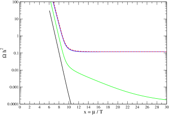
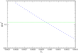
Figure 11: Left: The relic DM abundances, $\Omega h^{2}\leavevmode\nobreak\ (\mbox{red}),\leavevmode\nobreak\ \Omega_{1}h^{2}=\Omega_{\eta}h^{2}\leavevmode\nobreak\ (\mbox{black}),\leavevmode\nobreak\ 4\Omega_{2}h^{2}=4\Omega_{K}h^{2}\leavevmode\nobreak\ (\mbox{green})$ and $3\Omega_{3}h^{2}=3\Omega_{\pi}h^{2}\leavevmode\nobreak\ (\mbox{blue})$, as a function of the inverse temperature $x=\mu/T$ for the parameter values (73). Though $\tilde{\eta}$ is almost in thermal equilibrium, its presence is essential for the $\tilde{K}$ and $\tilde{\pi}$ numbers to decrease as $x$ decreases. In the end the relic abundance of $\tilde{\pi}$ dominates. Right: The total relic abundance $\Omega h^{2}$ as a function of $y_{1}(=y_{2})$ for $y_{3}=0.00424$, where the other parameters are fixed as (73).

IV.4 Indirect and Direct Detection of Dark Matter

IV.4.1 Monochromatic $\gamma$-ray line from DM annihilation

As we can see from Fig. 9, two DM particles can annihilate into two $\gamma$s. Therefore, the charge $Q$ of the hidden fermions can be constrained from the $\gamma$-ray observations Ackermann:2012qk ; Gustafsson:2013fca ; Abramowski:2013ax . Since in the $SU(2)_{V}$ case the relic abundance of the $\tilde{\pi}$ dark matter is dominant, we consider here only its annihilation into two $\gamma$s. We will take into account only the s-wave contribution to the annihilation cross section, and correspondingly we assume that $p=p^{\prime}=(m_{\tilde{\pi}},\bf 0)$ and that the photon momenta take the form $k=(m_{\tilde{\pi}},\bf k)$ and $k^{\prime}=(m_{\tilde{\pi}},-\bf k)$ with their polarization tensors $\epsilon(k)=(0,\mbox{\boldmath$\epsilon$}(k))$ and $\epsilon(k^{\prime})=(0,\mbox{\boldmath$\epsilon$}(k^{\prime}))$ satisfying

$$0 = \epsilon(k)\cdot k=\epsilon(k)\cdot k^{\prime}=\epsilon(k)\cdot p=\epsilon(k)\cdot p^{\prime}\leavevmode\nobreak\ ,$$

$$0 = \epsilon(k^{\prime})\cdot k=\epsilon(k^{\prime})\cdot k^{\prime}=\epsilon(k^{\prime})\cdot p=\epsilon(k^{\prime})\cdot p^{\prime}\leavevmode\nobreak\ ,$$ (74)

respectively.

To compute the annihilation rate we use the effective interaction (IV.2). We find that the annihilation amplitude can be written as

$$\Gamma_{\mu\nu}(a\leavevmode\nobreak\ b) \simeq G_{\pi^{2}\gamma^{2}}\left(k\cdot k^{\prime}g_{\mu\nu}-k_{\mu}k^{\prime}_{\nu}\right)\times\left\{\begin{array}[]{cc}&a\leavevmode\nobreak\ b\\ 1&\gamma\gamma\\ -t_{W}&\gamma\leavevmode\nobreak\ Z\\ t_{W}^{2}&Z\leavevmode\nobreak\ Z\end{array}\leavevmode\nobreak\ ,\right.$$ (79)

where $G_{\pi^{2}\gamma^{2}}$ is given in (60).

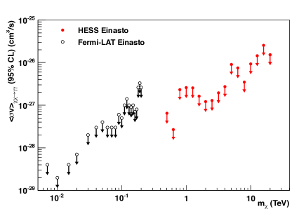
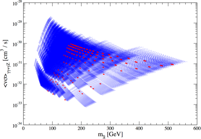
Figure 12: Left: The Fermi Lat Gustafsson:2013fca (black) and HESSAckermann:2012qk (red) upper bounds on the velocity-averaged DM annihilation cross section for monochromatic $\gamma$-ray lines, where this graph is taken from Ackermann:2012qk . Right: The velocity-averaged DM annihilation cross section $\langle v\sigma\rangle_{\gamma\gamma+\gamma Z}$ as a function of $m_{\tilde{\pi}}$ with $Q=1/3$. Since $\langle v\sigma\rangle_{\gamma\gamma+\gamma Z}$ is proportional to $Q^{4}$, our calculations can be simply extended to the case of an arbitrary $Q$. The red points are those for the $SU(3)_{V}$ case (9).

Then (the s-wave part of) the corresponding velocity-averaged annihilation cross sections are

$$\langle v\sigma(\tilde{\pi}\tilde{\pi}\to a\leavevmode\nobreak\ b)\rangle = \frac{G_{\pi^{2}\gamma^{2}}m_{\tilde{\pi}}^{2}}{4\pi}\times\left\{\begin{array}[]{cc}&a\leavevmode\nobreak\ b\\ (1/2)&\gamma\leavevmode\nobreak\ \gamma\\ t_{W}^{2}(1-m_{Z}^{2}/4m_{\tilde{\pi}}^{2})&\gamma\leavevmode\nobreak\ Z\\ (3/4)t_{W}^{4}(1-m_{Z}^{2}/m_{\tilde{\pi}}^{2})^{1/2}&Z\leavevmode\nobreak\ Z\end{array}\leavevmode\nobreak\ .\right.$$ (84)

The energy $E_{\gamma}$ of $\gamma$-ray line produced by the annihilation into $\gamma Z$ is $m_{\tilde{\pi}}(1-m_{Z}^{2}/4m_{\tilde{\pi}}^{2})$. In practice, however, due to finite detector energy resolution this line cannot be distinguished from the $E_{\gamma}=m_{\tilde{\pi}}$ line. Therefore, we simply add both cross sections. So we compute $\langle v\sigma\rangle_{\gamma\gamma+\gamma Z}=\langle v\sigma(\tilde{\pi}\tilde{\pi}\to\gamma\gamma)\rangle+\langle v\sigma(\tilde{\pi}\tilde{\pi}\to\gamma Z)\rangle$ with $Q=1/3$ as a function of $m_{\tilde{\pi}}$ for different values of $\lambda_{H},\leavevmode\nobreak\ \lambda_{S}$ and $\lambda_{HS}$, which is shown in Fig. 12 (right), where $\Omega h^{2}$ is required to be consistent with the PLANCK experiment at $4\sigma$ level Planck:2015xua . As we see from Fig. 12 (right) the velocity- averaged annihilation cross section is mostly less than $10^{-29}\leavevmode\nobreak\ \mbox{cm}^{3}/\mbox{s}$ in the parameter space we are considering, and consequently the Fermi LAT and HESS constraints given in Fig. 12 (left) are well satisfied. The red points are those for the $SU(3)_{V}$ (9) case.

The differential $\gamma$-ray flux is given by

$$\frac{d\Phi}{dE_{\gamma}} \propto \langle v\sigma\rangle_{\gamma\gamma}\frac{dN^{\gamma\gamma}}{dE_{\gamma}}+\langle v\sigma\rangle_{\gamma Z}\frac{dN^{\gamma z}}{dE_{\gamma Z}}\simeq\langle v\sigma\rangle_{\gamma\gamma+\gamma Z}\leavevmode\nobreak\ \delta(E_{\gamma}-m_{\rm DM})\leavevmode\nobreak\ .$$ (85)

Prospects observing such line spectrum is discussed in detail in Bringmann:2007nk ; Bertone:2009cb ; Laha:2012fg . Obviously, with an increasing energy resolution the chance for the observation increases. Observations of monochromatic $\gamma$-ray lines of energies of $O(100)$ GeV not only fix the charge of the hidden sector fermions, but also yields a first experimental hint on the hidden sector.

IV.4.2 Direct Detection of Dark Matter

As we can see from Fig. 11 (left), the relic abundance of the $\tilde{K}$ dark matter is about three orders of magnitude smaller than that of the $\tilde{\pi}$ dark matter. Therefore, we consider only the spin-independent elastic cross section $\sigma_{SI}$ of $\tilde{\pi}$ off the nucleon. The subprocess is the left diagram in Fig. 13 (left), where $\bullet$ is the localized one-loop contribution (53), and we ignore the right diagram. The result of Barbieri:2006dq can be used to find

$$\sigma_{SI} = \frac{{Z_{\tilde{\pi}}^{2}}}{\pi}G_{\pi^{2}S}^{2}\left[\frac{\hat{f}m_{N}}{2v_{h}m_{\tilde{\pi}}}\frac{\sin 2\theta}{2}\left(\frac{1}{m_{h}^{2}}-\frac{1}{m_{S}^{2}}\right)\right]^{2}\left(\frac{m_{N}m_{\tilde{\pi}}}{m_{N}+m_{\tilde{\pi}}}\right)^{2}\leavevmode\nobreak\ ,$$ (86)

where $G_{\pi^{2}S}$ is given in (53), $m_{N}$ is the nucleon mass, and $\hat{f}\sim 0.3$ stems from the nucleonic matrix element Ellis:2000ds . We assume $|\cos\theta|\gtrsim 0.9$ to satisfy the LHC constraint, where $\theta$ is the $h-S$ mixing angle. In Fig. 13 (right) we show in the $m_{\tilde{\pi}}\mbox{-}\sigma_{SI}$ plane the area in which $\Omega h^{2}=0.12\pm 0.01\leavevmode\nobreak\ (4\sigma)$ Planck:2015xua is satisfied. The predicted values of $\sigma_{SI}$ for $m_{\tilde{\pi}}\mathrel{\mathchoice{\vbox{\offinterlineskip\halign{$\m@th\displaystyle\hfil#\hfil$\cr>\crcr\sim\crcr} }}{\vbox{\offinterlineskip\halign{$\m@th\textstyle\hfil#\hfil$\cr>\crcr\sim\crcr} }}{\vbox{\offinterlineskip\halign{$\m@th\scriptstyle\hfil#\hfil$\cr>\crcr\sim\crcr} }}{\vbox{\offinterlineskip\halign{$\m@th\scriptscriptstyle\hfil#\hfil$\cr>\crcr\sim\crcr} }}}150$ GeV is too small even for the future direct DM detection experiment such as XENON1T, whose sensitivity is of $O(10^{-47})$ $\mbox{cm}^{2}$ Aprile:2012zx . The smallness of $\sigma_{SI}$ results from the smallness of the coupling $G_{\pi^{2}S}$, whose smallness comes from small Yukawa coupling $y_{1}$ and the accidental cancellation between the left and right diagrams in Fig. 7. The red points are those for the $SU(3)_{V}$ (9) case. We recall that the realistic parameter space for the $SU(2)_{V}$ case is not continuously connected to that for the $SU(3)_{V}$ case, as one could see from Fig. 11 (right), in which $y_{1}=y_{3}$ has to be satisfied for the $SU(3)_{V}$ case.

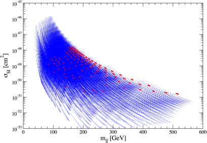
Figure 13: Left: Subdiagrams contributing to the spin-independent elastic cross section $\sigma_{SI}$ off the nucleon. Since the relic abundance of $\tilde{K}$ is negligibly small, the right diagram does not contribute. Right: The spin-independent elastic cross section $\sigma_{SI}$ of $\tilde{\pi}$ as a function of $m_{\tilde{\pi}}$. The red points are those for the $SU(3)_{V}$ case (9). The result should be compared with the XENON1T sensitivity of $O(10^{-47})\leavevmode\nobreak\ \mbox{cm}^{2}$ Aprile:2012zx .

If the relic abundance of the $\tilde{K}$ dark matter were of $O(0.1)$, the non-zero $\tilde{K}^{0}\mbox{-}\tilde{\bar{K}}^{0}\mbox{-}\gamma/Z$ and $\tilde{K}^{+}\mbox{-}\tilde{K}^{-}\mbox{-}\gamma/Z$ couplings shown in Fig. 13 would lead to a serious problem. Fortunately, the effective coupling is very small as we have already noticed: $m_{\tilde{K}}^{2}G_{K^{+}K^{-}\gamma}\sim 10^{-6}$, where this coupling for $\tilde{\pi}$ vanishes in the $SU(2)_{V}$ case.

Note that because an accidental $U(1)_{V}$ (the hidden baryon number), not only the DM candidates, but also the lightest hidden baryons are stable. The hidden mesons in our model are neutral, while the charge of the hidden baryons $\tilde{b}$ formed by three hidden fermions is $Q_{\tilde{b}}=3\times Q$. Let us roughly estimate the amount of relic stable hidden baryons and anti-baryons in the Universe, where we assume that the hidden proton and neutron are the lightest baryons in the $SU(2)_{V}$ case (8). As the hidden sector is described by a scaled-up QCD, the hidden meson-baryon coupling $G_{\phi B\bar{B}}$ is approximately the same as in QCD, i.e. $G_{\phi B\bar{B}}\sim 13$, which is independent of $Q$. Using this fact, we can estimate $Y_{\tilde{b}}=n_{\tilde{b}}/s$ and obtain $Y_{\tilde{b}}\leavevmode\nobreak\ \simeq(0.4,\leavevmode\nobreak\ 6,\leavevmode\nobreak\ 9)\times 10^{-16}$ for $m_{\tilde{b}}=1,\leavevmode\nobreak\ 5$ and $8$ TeV, respectively. There are severe constraints on $Y_{\tilde{b}}$. The most severe constraints exist for $Q_{\tilde{b}}=1$, which come from the search of heavy isotopes in sea water Agashe:2014kda and also from its influence on the large scale structure formation of the Universe Kohri:2009mi . We therefore conclude that $Q_{\tilde{b}}=1$, i.e. $Q=1/3$ is ruled out. Another severe cosmological constraint is due to catalyzed BBN Pospelov:2006sc , which gives $Y_{\tilde{b}}\mathrel{\mathchoice{\vbox{\offinterlineskip\halign{$\m@th\displaystyle\hfil#\hfil$\cr<\crcr\sim\crcr} }}{\vbox{\offinterlineskip\halign{$\m@th\textstyle\hfil#\hfil$\cr<\crcr\sim\crcr} }}{\vbox{\offinterlineskip\halign{$\m@th\scriptstyle\hfil#\hfil$\cr<\crcr\sim\crcr} }}{\vbox{\offinterlineskip\halign{$\m@th\scriptscriptstyle\hfil#\hfil$\cr<\crcr\sim\crcr} }}}2\times 10^{-15}$ Pospelov:2008ta (see also Hamaguchi:2007mp ). The CMB constraint based on the Planck data is $\Omega_{\tilde{b}}h^{2}\mathrel{\mathchoice{\vbox{\offinterlineskip\halign{$\m@th\displaystyle\hfil#\hfil$\cr<\crcr\sim\crcr} }}{\vbox{\offinterlineskip\halign{$\m@th\textstyle\hfil#\hfil$\cr<\crcr\sim\crcr} }}{\vbox{\offinterlineskip\halign{$\m@th\scriptstyle\hfil#\hfil$\cr<\crcr\sim\crcr} }}{\vbox{\offinterlineskip\halign{$\m@th\scriptscriptstyle\hfil#\hfil$\cr<\crcr\sim\crcr} }}}0.001$ Dolgov:2013una , which can be satisfied in our model if $m_{\tilde{b}}\mathrel{\mathchoice{\vbox{\offinterlineskip\halign{$\m@th\displaystyle\hfil#\hfil$\cr<\crcr\sim\crcr} }}{\vbox{\offinterlineskip\halign{$\m@th\textstyle\hfil#\hfil$\cr<\crcr\sim\crcr} }}{\vbox{\offinterlineskip\halign{$\m@th\scriptstyle\hfil#\hfil$\cr<\crcr\sim\crcr} }}{\vbox{\offinterlineskip\halign{$\m@th\scriptscriptstyle\hfil#\hfil$\cr<\crcr\sim\crcr} }}}6$ TeV. (See also Langacker:2011db in which the constraints in the $Q_{\tilde{b}}$-DM mass plane are given, where these constraints are satisfied in a wide area of the parameter space of the present model.).

In most of our analyses on DM here we have used $Q=1/3$. The relic abundances of DMs depend on $Q$, because the decay rate of the neutral would-be DM $\eta$ depends on $Q$. The change of $Q$ can be compensated by varying the ratio of $y_{3}$ to $y_{1}=y_{2}$, as far as the difference of two hypercharges are not very much different. As for the indirect detection of DM, the annihilation cross section into two $\gamma$s (84) being proportional to $Q^{4}$ should be multiplied with $(3Q)^{4}$ for $Q$ different from $1/3$. The spin-independent elastic cross section $\sigma_{SI}$ (86) is independent on $Q$. This means that our basic results obtained in this paper can be simply extended to the case with $Q$ different from $1/3$.

V Conclusion

We have considered a QCD-like hidden sector model Hur:2007uz ; Hur:2011sv ; Heikinheimo:2013fta ; Holthausen:2013ota , in which dynamical chiral symmetry breaking generates a mass scale. This generated scale is transmitted to the SM sector via a real SM singlet scalar $S$ to trigger spontaneous breaking of EW gauge symmetry Hur:2007uz ; Hur:2011sv . Because the SM is extended in a classically scale invariant way, ”Mass without mass” wheeler ; wilczek is realized in this model. Since chiral symmetry is dynamically broken, there exist NG bosons, which are massive because the coupling of $S$ with the hidden sector fermions breaks explicitly the $SU(n_{f})_{L}\times SU(n_{f})_{R}$ chiral symmetry down to one of its diagonal subgroups. The mass scale of these NG bosons is calculable once the strength of this coupling and the scale of the QCD-like hidden sector are given. The smallest subgroup is the Cartan subalgebra $U(1)^{n_{f}-1}$. Because of this (accidentally) unbroken subgroup, the NG bosons charged under $U(1)^{n_{f}-1}$ are stable: There exist at least $n_{f}^{2}-n_{f}$ DM candidates. We have restricted ourselves to $n_{c}=n_{f}=3$, because in this case we can relate using hadrons the independent parameters of the NJL model, which we have used as a low-energy effective theory for the hidden sector. There are three possibilities: (i) $U(1)_{\tilde{B}^{\prime}}\times U(1)_{\tilde{B}}$, (ii) $SU(2)_{V}\times U(1)_{\tilde{B}}$, and (iii) $SU(3)_{V}$, where the possibility (iii) has been studied in Holthausen:2013ota ; Kubo:2014ida . It turns out that the first case (i) is unrealistic, unless this case is very close to (ii) or (iii), or/and the hypercharge $Q$ of the hidden fermions is tiny. This is because the lightest NG boson is neutral under $U(1)_{\tilde{B}^{\prime}}\times U(1)_{\tilde{B}}$ so that it can decay into two $\gamma$s and the stable DM candidates annihilate into them immediately. Therefore, we have mainly studied the case (ii) with $y_{1}=y_{2}<y_{3}$. In this case the unstable NG boson is $\tilde{\eta}$ (the heaviest among the pseudo NG bosons) and can decay into two $\gamma$s. The annihilation cross section into the SM particles via the singlet $S$ is very much suppressed, except in the resonance region in the s-channel annihilation diagram of DM. However, we have found another mechanism for the stable DMs to annihilate: If $y_{3}$ does not differ very much from $y_{1}=y_{2}$, the differences among $m_{\tilde{\pi}},m_{\tilde{K}}$ and $m_{\tilde{\eta}}$ are small. At finite temperature the inverse DM conversions (which are kinematically forbidden at zero temperature) can become operative, because the DM conversions cross sections are large $\sim 10^{-5}\leavevmode\nobreak\ \mbox{GeV}^{-2}$. Consequently, the realistic parameter space of the case (ii) is significantly larger than that of the case (iii), which has been obtained in Holthausen:2013ota ; Kubo:2014ida .

With a non-zero $Q$ the hidden sector is doubly connected with the SM sector; we have a bright hidden sector at hand. The connection via photon and $Z$ opens possibilities to probe the hidden sector at collider experiments such as $e^{+}e^{-}$ collision Fujii . In particular, the would-be DM, $\tilde{\eta}$, can decay into two $\gamma$s, which would give a smoking-gun event.

Acknowledgements: We thank S. Matsumoto and H. Takano for useful discussions. The work of M. A. is supported in part by the Grant-in-Aid for Scientific Research (Grant Nos. 25400250 and 26105509).

Appendix A The NJL Lagrangian in the self-consistent mean field (SCMF) approximation

Here we consider the NJL Lagrangian ${\cal L}_{\rm NJL}$ (19) in the SCMF approximation Hatsuda:1994pi . In the SCMF approximation one splits up the NJL Lagrangian (19) into the sum

$$\mathcal{L}_{\rm NJL} = \mathcal{L}_{0}+\mathcal{L}_{I}\leavevmode\nobreak\ ,$$ (87)

where $\mathcal{L}_{I}$ is normal ordered (i.e. $\langle 0|\mathcal{L}_{I}|0\rangle=0$), and $\mathcal{L}_{0}$ contains at most fermion bilinears which are not normal ordered. We find that ${\cal L}_{0}$ can be written as

$${\cal L}_{0} = {\cal L}_{K}+{\cal L}_{D}+{\cal L}_{M}\leavevmode\nobreak\ ,$$ (88)

where

$${\cal L}_{K} = {\rm Tr}{\bar{\psi}}(i{\gamma}^{\mu}\partial_{\mu}+g^{\prime}Q{\gamma}^{\mu}B_{\mu}){\psi}-\Bigl{(}\tilde{\sigma}_{1}+y_{1}S-\frac{G_{D}}{8G^{2}}\tilde{\sigma}_{2}\tilde{\sigma}_{3}\Bigr{)}\bar{\psi_{1}}\psi_{1}$$

$$-\Bigl{(}\tilde{\sigma}_{2}+y_{2}S-\frac{G_{D}}{8G^{2}}\tilde{\sigma}_{1}\tilde{\sigma}_{3}\Bigr{)}\bar{\psi_{2}}\psi_{2}-\Bigl{(}\tilde{\sigma}_{3}+y_{3}S-\frac{G_{D}}{8G^{2}}\tilde{\sigma}_{1}\tilde{\sigma}_{2}\Bigr{)}\bar{\psi_{3}}\psi_{3}$$

$$-i\Bigl{[}\tilde{\pi}^{0}+\frac{1}{\sqrt{3}}\tilde{\eta}^{8}+\sqrt{\frac{2}{3}}\tilde{\eta}^{0}-\frac{G_{D}}{8G^{2}}\Bigl{(}\tilde{\sigma}_{3}\tilde{\pi}^{0}+\frac{1}{\sqrt{3}}(2\tilde{\sigma}_{2}-\tilde{\sigma}_{3})\tilde{\eta}^{8}-\sqrt{\frac{2}{3}}(\tilde{\sigma}_{2}+\tilde{\sigma}_{3})\tilde{\eta}^{0}\Bigr{)}\Bigr{]}\bar{\psi_{1}}{\gamma}_{5}\psi_{1}$$

$$-i\Bigl{[}-\tilde{\pi}^{0}+\frac{1}{\sqrt{3}}\tilde{\eta}^{8}+\sqrt{\frac{2}{3}}\tilde{\eta}^{0}-\frac{G_{D}}{8G^{2}}\Bigl{(}-\tilde{\sigma}_{3}\tilde{\pi}^{0}+\frac{1}{\sqrt{3}}(2\tilde{\sigma}_{1}-\tilde{\sigma}_{3})\tilde{\eta}^{8}-\sqrt{\frac{2}{3}}(\tilde{\sigma}_{1}+\tilde{\sigma}_{3})\tilde{\eta}^{0})\Bigr{)}\Bigr{]}\bar{\psi_{2}}{\gamma}_{5}\psi_{2}$$

$$-i\sqrt{2}\tilde{\pi}^{+}\Bigl{(}1-\frac{G_{D}}{8G^{2}}\tilde{\sigma}_{3}\Bigr{)}{\bar{\psi_{1}}}{\gamma}_{5}\psi_{2}-i\sqrt{2}\tilde{\pi}^{-}\Bigl{(}1-\frac{G_{D}}{8G^{2}}\tilde{\sigma}_{3}\Bigr{)}{\bar{\psi_{2}}}{\gamma}_{5}\psi_{1}$$

$$-i\sqrt{2}\tilde{K}^{+}\Bigl{(}1-\frac{G_{D}}{8G^{2}}\tilde{\sigma}_{2}\Bigr{)}{\bar{\psi_{1}}}{\gamma}_{5}\psi_{3}-i\sqrt{2}\tilde{K}^{-}\Bigl{(}1-\frac{G_{D}}{8G^{2}}\tilde{\sigma}_{2}\Bigr{)}{\bar{\psi_{3}}}{\gamma}_{5}\psi_{1}$$

$$-i\sqrt{2}\tilde{K}^{0}\Bigl{(}1-\frac{G_{D}}{8G^{2}}\tilde{\sigma}_{1}\Bigr{)}{\bar{\psi_{2}}}{\gamma}_{5}\psi_{3}-i\sqrt{2}\bar{\tilde{K}}^{0}\Bigl{(}1-\frac{G_{D}}{8G^{2}}\tilde{\sigma}_{1}\Bigr{)}{\bar{\psi_{3}}}{\gamma}_{5}\psi_{2}$$

$$-i\Bigl{[}-\frac{2}{\sqrt{3}}\tilde{\eta}^{8}+\sqrt{\frac{2}{3}}\tilde{\eta}^{0}-\frac{G_{D}}{8G^{2}}\Bigl{(}(\tilde{\sigma}_{1}-\tilde{\sigma}_{2})\tilde{\pi}^{0}-\frac{1}{\sqrt{3}}(\tilde{\sigma}_{1}+\tilde{\sigma}_{2})\tilde{\eta}^{8}-\sqrt{\frac{2}{3}}(\tilde{\sigma}_{1}+\tilde{\sigma}_{2})\tilde{\eta}^{0}\Bigr{)}\Bigr{]}{\bar{\psi_{3}}}{\gamma}_{5}\psi_{3}\leavevmode\nobreak\ ,$$

$${\cal L}_{D} = \frac{G_{D}}{8G^{2}}\Biggl{[}\Bigl{(}2\tilde{K}^{0}\bar{\tilde{K}^{0}}-\frac{2}{\sqrt{3}}\tilde{\pi}^{0}\tilde{\eta}^{8}+\frac{2}{3}({\tilde{\eta}^{8}})^{2}-\frac{2}{3}({\tilde{\eta}^{0}})^{2}\Bigr{)}\bar{\psi_{1}}\psi_{1}-\Bigl{(}2\sqrt{\frac{2}{3}}\tilde{\pi}^{+}\tilde{\eta}^{8}+2\tilde{K}^{+}\bar{\tilde{K}^{0}}\Bigr{)}\bar{\psi_{1}}\psi_{2}$$ (90)

$$-\Bigl{(}2\sqrt{\frac{2}{3}}\tilde{\pi}^{-}\tilde{\eta}^{8}+2\tilde{K}^{-}{\tilde{K}^{0}}\Bigr{)}\bar{\psi_{2}}\psi_{1}+\Bigl{(}2\tilde{K}^{+}\tilde{K}^{-}+\frac{2}{\sqrt{3}}\tilde{\pi}^{0}\tilde{\eta}^{8}+\frac{2}{3}({\tilde{\eta}^{8}})^{2}-\frac{2}{3}({\tilde{\eta}^{0}})^{2}\Bigr{)}\bar{\psi_{2}}\psi_{2}$$

$$-\Bigl{(}2\tilde{\pi}^{+}\tilde{K}^{0}+\sqrt{2}\tilde{K}^{+}(\tilde{\pi}^{0}-\frac{1}{\sqrt{3}}\tilde{\eta}^{8})\Bigr{)}\bar{\psi_{1}}\psi_{3}-\Bigl{(}2\tilde{\pi}^{-}\bar{\tilde{K}^{0}}+\sqrt{2}\tilde{K}^{-}(\tilde{\pi}^{0}-\frac{1}{\sqrt{3}}\tilde{\eta}^{8})\Bigr{)}\bar{\psi_{3}}\psi_{1}$$

$$-\Bigl{(}2\tilde{\pi}^{-}\tilde{K}^{+}-\sqrt{2}\tilde{K}^{0}(\tilde{\pi}^{0}+\frac{1}{\sqrt{3}}\tilde{\eta}^{8}\bigr{)}\Bigr{)}\bar{\psi_{2}}\psi_{3}-\Bigl{(}2\tilde{\pi}^{+}\tilde{K}^{-}-\sqrt{2}\bar{\tilde{K}}^{0}(\tilde{\pi}^{0}+\frac{1}{\sqrt{3}}\tilde{\eta}^{8})\Bigr{)}\bar{\psi_{3}}\psi_{2}$$

$$+\Bigl{(}2\tilde{\pi}^{+}\tilde{\pi}^{-}+({\tilde{\pi}^{0}})^{2}-\frac{1}{3}(\tilde{\eta}^{8})^{2}-\frac{2}{3}(\tilde{\eta}^{0})^{2}\Bigr{)}\bar{\psi_{3}}\psi_{3}$$

$$+\sqrt{\frac{2}{3}}\tilde{\eta}^{0}\Bigl{\{}(\tilde{\pi}^{0}+\frac{1}{\sqrt{3}}\tilde{\eta}^{8})\bar{\psi_{1}}\psi_{1}+\sqrt{2}\tilde{\pi}^{+}{\bar{\psi_{1}}}\psi_{2}+\sqrt{2}\tilde{K}^{+}{\bar{\psi_{1}}}\psi_{3}+\sqrt{2}\tilde{\pi}^{-}{\bar{\psi_{2}}}\psi_{1}$$

$$+(-\tilde{\pi}^{0}+\frac{1}{\sqrt{3}}\tilde{\eta}^{8})\bar{\psi_{2}}\psi_{2}+\sqrt{2}\tilde{K}^{0}{\bar{\psi_{2}}}\psi_{3}+\sqrt{2}\tilde{K}^{-}{\bar{\psi_{3}}}\psi_{1}+\sqrt{2}\bar{\tilde{K}^{0}}{\bar{\psi_{3}}}\psi_{2}-\frac{2}{\sqrt{3}}\tilde{\eta}^{8}{\bar{\psi_{3}}}\psi_{3}\Bigr{\}}\Biggr{]}\leavevmode\nobreak\ ,$$

$${\cal L}_{M} = -\frac{1}{8G}\Biggl{(}\sum_{i=1}^{3}\tilde{\sigma}_{i}^{2}+2(\tilde{\eta}^{0})^{2}+4\tilde{\pi}^{+}\tilde{\pi}^{-}+4\tilde{K}^{+}\tilde{K}^{-}+4\tilde{K}^{0}\bar{\tilde{K}}^{0}+2(\tilde{\pi}^{0})^{2}+2(\tilde{\eta}^{8})^{2}\Biggr{)}$$ (91)

$$+\frac{G_{D}}{16G^{3}}\Biggl{[}\tilde{\sigma}_{1}\tilde{\sigma}_{2}\tilde{\sigma}_{3}+\tilde{\sigma}_{1}\Bigl{(}2\tilde{K}^{0}\bar{\tilde{K}}^{0}+\frac{2}{3}(\tilde{\eta}^{8})^{2}-\frac{2}{3}(\tilde{\eta}^{0})^{2}-\frac{2}{\sqrt{3}}\tilde{\pi}^{0}\tilde{\eta}^{8}+\sqrt{\frac{2}{3}}\tilde{\eta}^{0}\tilde{\pi}^{0}+\frac{\sqrt{2}}{3}\tilde{\eta}^{0}\tilde{\eta}^{8}\Bigr{)}$$

$$+\tilde{\sigma}_{2}\Bigl{(}2\tilde{K}^{+}\tilde{K}^{-}+\frac{2}{3}(\tilde{\eta}^{8})^{2}-\frac{2}{3}(\tilde{\eta}^{0})^{2}+\frac{2}{\sqrt{3}}\tilde{\pi}^{0}\tilde{\eta}^{8}-\sqrt{\frac{2}{3}}\tilde{\eta}^{0}\tilde{\pi}^{0}+\frac{\sqrt{2}}{3}\tilde{\eta}^{0}\tilde{\eta}^{8}\Bigr{)}$$

$$+\tilde{\sigma}_{3}\Bigl{(}2\tilde{\pi}^{+}\tilde{\pi}^{-}+(\tilde{\pi}^{0})^{2}-\frac{1}{3}(\tilde{\eta}^{8})^{2}-\frac{2}{3}(\tilde{\eta}^{0})^{2}-\frac{2\sqrt{2}}{3}\tilde{\eta}^{0}\tilde{\eta}^{8}\Bigr{)}\Biggr{]}\leavevmode\nobreak\ .$$

Here $\tilde{\eta}^{0}$ stands for $\phi_{0}$, and the meson fields are defined in (4).

Appendix B Determination of the NJL parameters $G,\,G_{D}$ and $\Lambda$

As in Holthausen:2013ota we apply the NJL Lagrangian (88) with $g^{\prime}=0$ to describe the real hadrons, where we assume $SU(2)_{V}$ and replace $y_{i}S$ by the current quark masses, i.e. $y_{1}S=y_{2}S\to m_{u}\leavevmode\nobreak\ ,\leavevmode\nobreak\ y_{3}S\to m_{s}$. Then we compute the real meson masses $m_{\pi},m_{K},m_{\eta},m_{\eta^{\prime}}$ and decay constants $f_{\pi},f_{K}$.

We obtain the following inverse meson propagators:

$$\Gamma_{\pi^{\pm}}({p^{2}}) = \Gamma_{{\pi^{0}}}(p^{2})$$ (92)

$$= -\frac{1}{2G}+\frac{G_{D}}{8G^{3}}\sigma_{3}+\Bigl{(}1-\frac{G_{D}}{8G^{2}}\sigma_{3}\Bigr{)}^{2}2n_{c}I_{\phi^{2}}^{A}(p^{2},m_{1},m_{1})+\frac{G_{D}}{G^{2}}n_{c}I_{\phi^{2}}^{B}(m_{3})\leavevmode\nobreak\ ,$$

$$\Gamma_{K^{\pm}}({p^{2}}) = \Gamma_{\bar{K^{0}}K^{0}}(p^{2})$$ (93)

$$= -\frac{1}{2G}+\frac{G_{D}}{8G^{3}}\sigma_{1}+\Bigl{(}1-\frac{G_{D}}{8G^{2}}\sigma_{1}\Bigr{)}^{2}2n_{c}I_{\phi^{2}}^{A}(p^{2},m_{1},m_{3})+\frac{G_{D}}{G^{2}}n_{c}I_{\phi^{2}}^{B}(m_{1})\leavevmode\nobreak\ ,$$

$$\Gamma_{\eta}^{8}(p^{2}) = -\frac{1}{2G}+\frac{G_{D}}{6G^{3}}(\sigma_{1}-\frac{1}{4}\sigma_{3})+\frac{2}{3}\Bigl{(}1-\frac{G_{D}}{8G^{2}}(2\sigma_{1}-\sigma_{3})\Bigr{)}^{2}n_{c}I_{\phi^{2}}^{A}(p^{2},m_{1},m_{1})$$ (94)

$$+ \frac{4}{3}\Bigl{(}1-\frac{G_{D}}{8G^{2}}\sigma_{1}\Bigr{)}^{2}n_{c}I_{\phi^{2}}^{A}(p^{2},m_{3},m_{3})+\frac{4G_{D}}{3G^{2}}n_{c}I_{\phi^{2}}^{B}(m_{1})-\frac{G_{D}}{3G^{2}}n_{c}I_{\phi^{2}}^{B}(m_{3})\leavevmode\nobreak\ ,$$

$$\Gamma_{\eta}^{0}(p^{2}) = -\frac{1}{2G}-\frac{G_{D}}{12G^{3}}\Big{(}2\sigma_{1}+\sigma_{3}\Bigr{)}+\Bigl{(}1+\frac{G_{D}}{8G^{2}}(\sigma_{1}+\sigma_{3})\Bigr{)}^{2}\frac{4}{3}n_{c}I_{\phi^{2}}^{A}(p^{2},m_{1},m_{1})$$ (95)

$$+ \Bigl{(}1+\frac{G_{D}}{4G^{2}}\sigma_{1}\Bigr{)}^{2}\frac{2}{3}n_{c}I_{\phi^{2}}^{A}(p^{2},m_{3},m_{3})-\frac{2G_{D}}{3G^{2}}n_{c}\Big{(}2I_{\phi^{2}}^{B}(m_{1})+I_{\phi^{2}}^{B}(m_{3})\Bigr{)}\leavevmode\nobreak\ ,$$

$$\Gamma_{{\eta}^{8}{\eta}^{0}}(p^{2}) = \frac{\sqrt{2}G_{D}}{24G^{3}}(\sigma_{1}-\sigma_{3})+\frac{2\sqrt{2}}{3}\biggl{(}1-\frac{G_{D}}{8G^{2}}(2\sigma_{1}-\sigma_{3})\biggr{)}\biggl{(}1+\frac{G_{D}}{8G^{2}}(\sigma_{1}+\sigma_{3})\biggr{)}n_{c}I_{\phi^{2}}^{A}(p^{2},m_{1},m_{1})$$ (96)

$$- \frac{2\sqrt{2}}{3}\biggl{(}1-\frac{G_{D}}{8G^{2}}\sigma_{1}\biggr{)}\biggl{(}1+{\frac{G_{D}}{8G^{2}}}(2\sigma_{1})\biggr{)}n_{c}I_{\phi^{2}}^{A}(p^{2},m_{3},m_{3})$$

$$+ \frac{\sqrt{2}G_{D}}{3G^{2}}n_{c}\bigl{(}I_{\phi^{2}}^{B}(m_{1})-I_{\phi^{2}}^{B}(m_{3})\bigr{)}\leavevmode\nobreak\ ,$$

where the integrals $I_{\phi^{2}}^{A}(p^{2},m_{a},m_{b})$ and $I_{\phi^{2}}^{B}(m)$ are defined in appendix (103), and

$$m_{1}=m_{u}+\sigma_{1}-\frac{G_{D}}{8G^{2}}{\sigma_{1}}{\sigma_{3}}\leavevmode\nobreak\ ,\leavevmode\nobreak\ m_{3}=m_{s}+\sigma_{3}-\frac{G_{D}}{8G^{2}}{\sigma_{1}}^{2}\leavevmode\nobreak\ .$$ (97)

The pion and kaon masses are the zeros of the inverse propagators, i.e.

$$\Gamma_{\pi^{\pm}}(p^{2}={m_{\pi}}^{2})=0\leavevmode\nobreak\ ,\leavevmode\nobreak\ \Gamma_{K^{\pm}}(p^{2}={m_{K}}^{2})=0\leavevmode\nobreak\ ,$$ (98)

while the $\eta$ and $\eta^{\prime}$ meson masses are obtained from the zero eigenvalues of the real part of the $\eta^{8}-\eta^{0}$ mixing matrix. The wave function renormalization constants can be obtained from

$${Z_{\pi}}^{-1} = \frac{d\Gamma_{\pi^{\pm}}(p^{2})}{dp^{2}}{\biggl{|}}_{p^{2}={m_{\pi}}^{2}}\leavevmode\nobreak\ ,\leavevmode\nobreak\ {Z_{K}}^{-1}=\frac{d\Gamma_{K^{\pm}}(p^{2})}{dp^{2}}{\biggl{|}}_{p^{2}={m_{K}}^{2}}\leavevmode\nobreak\ ,$$ (99)

and the pion and kaon decay constants are defined as

$$<0|{\rm Tr}\bar{\psi}{\gamma}_{\mu}{\gamma}_{5}\frac{1}{2}(\sigma_{1}+i\sigma_{2}){\psi}|{\pi^{+}}(p)> = i\sqrt{2}f_{\pi}p_{\mu}\leavevmode\nobreak\ ,$$ (100)

$$<0|{\rm Tr}\bar{\psi}{\gamma}_{\mu}{\gamma}_{5}\frac{1}{2}(\sigma_{4}+i\sigma_{5}){\psi}|{K^{+}}(p)> = i\sqrt{2}f_{K}p_{\mu}\leavevmode\nobreak\ .$$ (101)

We use $m_{\pi},m_{K},m_{\eta},m_{\eta^{\prime}},f_{\pi}$ and $f_{K}$ to determine the QCD NJL parameters. The best fit values of the parameters are given in Table 2.

Parameter	$(2G^{\mathrm{QCD}})^{-1/2}$	$(-G_{D}^{\mathrm{QCD}})^{-1/5}$	$\Lambda^{\mathrm{QCD}}$	$m_{u}$	$m_{s}$
Value (MeV)	$361$	$406$	$930$	$5.95$	$163$

Table 2: Values of the QCD NJL parameters obtained by fitting the pion and kaon decay constants and the meson masses, where we have assumed the $SU(2)_{V}$ flavor symmetry.

In Table 3 we compare the meson masses and decay constants calculated in the NJL theory with the experimental values.

	Theory(MeV)	Experimental value(MeV)
$m_{\pi}$	$136$	$140(\pi^{\pm})\leavevmode\nobreak\ 135(\pi^{0})$
$m_{K}$	$499$	$494(K^{\pm})\leavevmode\nobreak\ 498(K^{0},\bar{K^{0}})$
$m_{\eta}$	$460$	$548$
$m_{\eta^{\prime}}$	$960$	$958$
$f_{\pi}$	$93$	$92(\pi^{-})$
$f_{K}$	$105$	$110(K^{-})$

Table 3: Comparison of the NJL values with the corresponding experimental values.

As we see from Table 3, the NJL $\eta$ mass is about $16$% smaller than the experimental value. This seems to be a general feature of the NJL theory Hatsuda:1994pi (see also Inagaki:2013hya ).

Appendix C One-loop Integrals

$\bullet$Vacuum energy
To compute the effective potential (24) we need the vacuum energy

$$I_{V}(m) = \int\frac{d^{4}k}{i(2\pi)^{4}}\ln\det(\not{k}-m)$$ (102)

$$= \frac{1}{16\pi^{2}}\left(\Lambda^{4}\ln\left(1+\frac{m^{2}}{\Lambda^{2}}\right)-m^{4}\ln\left(1+\frac{\Lambda^{2}}{m^{2}}\right)+m^{2}\Lambda^{2}\right)\leavevmode\nobreak\ .$$

$\bullet$Inverse propagator of dark matter
There are two types of diagrams which contribute to the inverse propagator of dark matter:

$$I_{\phi^{2}}^{A}(p^{2},m_{a},m_{b}) = \int\frac{d^{4}l}{i(2\pi)^{4}}\frac{\mbox{Tr}(\not{l}-\not{p}+m_{a})\gamma_{5}(\not{l}+m_{b})\gamma_{5}}{((l-p)^{2}-m_{a}^{2})(l^{2}-m_{b}^{2})},$$

$$I_{\phi^{2}}^{B}(m) = \int\frac{d^{4}k}{i(2\pi)^{4}}\frac{m}{(k^{2}-m^{2})}=-\frac{1}{16\pi^{2}}m\left[\Lambda^{2}-m^{2}\ln\left(1+\frac{\Lambda^{2}}{m^{2}}\right)\right]\leavevmode\nobreak\ .$$ (103)

These expressions are used to find DM masses and wave function renormalization constants given in (99), respectively.

$\bullet$$\phi\mbox{-}\phi\mbox{-}\gamma$ amplitude

$$I_{\phi^{2}\gamma}^{\mu}(p,p^{\prime},m_{a},m_{b})$$

$$=(-1)\int\frac{d^{4}l}{i(2\pi)^{4}}\frac{\mbox{Tr}(\not{l}+m_{a})\gamma_{5}(\not{l}-\not{p}^{\prime}+m_{b})\gamma^{\mu}(\not{l}+\not{p}+m_{b})\gamma_{5}}{((l+p)^{2}-m_{b}^{2})(l^{2}-m_{a}^{2})((l-p^{\prime})^{2}-m_{b}^{2})}\leavevmode\nobreak\ +(p\leftrightarrow p^{\prime},m_{a}\leftrightarrow m_{b}),$$

$$=-(p^{\mu}p^{\prime\nu}-p^{\prime\mu}p^{\nu})(p+p^{\prime})_{\nu}I_{\phi\gamma^{2}}(m_{a},m_{b})+\cdots$$ (104)

$\mbox{with}\leavevmode\nobreak\ p^{2}=p^{\prime 2}$, where $\cdots$ stands for higher order terms in the expansion of the external momenta, and

$$I_{\phi^{2}\gamma}(m_{a},m_{b}) = \frac{1}{8\pi^{2}}\frac{1}{(m_{a}^{2}-m_{b}^{2})^{2}(m_{a}+m_{b})^{2}}$$ (105)

$$\times\left(\frac{1}{2}(m_{a}-m_{b})(m_{a}^{3}+5m_{a}^{2}m_{b}+5m_{a}m_{b}^{2}+m_{b}^{3})\right.$$

$$\left.-\frac{1}{3}(m_{a}^{4}+3m_{a}^{3}m_{b}+m_{a}^{2}m_{b}^{2}+3m_{a}m_{b}^{3}+m_{b}^{4})\ln(m_{a}^{2}/m_{b}^{2})^{2}\right)\leavevmode\nobreak\ .$$

The effective $\phi\mbox{-}\phi\mbox{-}\gamma$ interaction Lagrangian is given in (37).

$\bullet$$\phi\mbox{-}\gamma\mbox{-}\gamma$ amplitude
The $\phi(p)\mbox{-}\gamma(k)\mbox{-}\gamma(k^{\prime})$ three-point function is needed to compute the decay $\tilde{\eta}$ into two $\gamma$s (Fig. 4):

$$I_{\phi\gamma^{2}}^{\mu\nu}(k,k^{\prime},m)$$

$$=(-1)\int\frac{d^{4}l}{i(2\pi)^{4}}\frac{\mbox{Tr}(\not{l}-\not{k}^{\prime}+m)\gamma^{\mu}(\not{l}+m)\gamma^{\nu}(\not{l}+\not{k}+m)\gamma_{5}}{((l+k)^{2}-m^{2})(l^{2}-m^{2})((l-k^{\prime})^{2}-m^{2})}\leavevmode\nobreak\ +(k\leftrightarrow k^{\prime},\mu\leftrightarrow\nu)\leavevmode\nobreak\$$

$$=\frac{i}{4\pi^{2}m}\epsilon^{\mu\nu\alpha\beta}k_{\alpha}k^{\prime}_{\beta}+\cdots$$ (106)

The amplitude is thanks to $\gamma_{5}$ gauge invariant even for a finite $\Lambda$, i.e.
$k_{\nu}I_{\phi\gamma^{2}}^{\mu\nu}(k,k^{\prime},m)=k^{\prime}_{\mu}I_{\phi\gamma^{2}}^{\mu\nu}(k,k^{\prime},m)=0$. The amplitude without $\gamma_{5}$ correspond to the $S(p)\mbox{-}\gamma(k)\mbox{-}\gamma(k^{\prime})$ three-point function, which we denote by $I_{0,S}^{\mu\nu}(k,k^{\prime},m)$. This amplitude is not gauge invariant so that we need to apply least subtraction method Kubo:2014ida . The subscript $0$ indicates that the amplitude is unsubtracted, and we denote the subtracted gauge-invariant one by $I_{S}^{\mu\nu}(k,k^{\prime},m)$. In Appendix C we demonstrate how to use least subtraction method for this case.

$\bullet$$\phi\mbox{-}\phi\mbox{-}\phi\mbox{-}\phi$ amplitude
The $\phi(p)\mbox{-}\phi(p^{\prime})\mbox{-}\phi^{\prime}(k)\mbox{-}\phi^{\prime}(k^{\prime})\mbox{-}$ four-point function is needed to compute the DM conversion cross section (diagrams of Fig. 5 ):

$$I^{A}_{\phi^{4}}(p,p^{\prime},k,k^{\prime},m_{a},m_{b},m_{c},m_{d})$$

$$=(-1)\int\frac{d^{4}l}{i(2\pi)^{4}}\frac{\mbox{Tr}(\not{l}+m_{a})\gamma_{5}(\not{l}-\not{p}^{\prime}+m_{b})\gamma_{5}(\not{l}+\not{p}-\not{k}+m_{c})\gamma_{5}(\not{l}+\not{p}+m_{d})\gamma_{5}}{(l^{2}-m_{a}^{2})((l-p^{\prime})^{2}-m_{b}^{2})((l+p-k)^{2}-m_{c}^{2})((l+p)^{2}-m_{d}^{2})}\leavevmode\nobreak\$$

$$+(p\leftrightarrow p^{\prime},k\leftrightarrow k^{\prime})\leavevmode\nobreak\ +(p\leftrightarrow p^{\prime})+(k\leftrightarrow k^{\prime})\leavevmode\nobreak\ ,$$ (107)

$$I^{B}_{\phi^{4}}(p,p^{\prime},m_{a},m_{b})$$

$$=(-1)\int\frac{d^{4}l}{i(2\pi)^{4}}\frac{\mbox{Tr}(\not{l}+m_{a})(\not{l}+\not{p}+\not{p}^{\prime}+m_{b})}{(l^{2}-m_{a}^{2})((l+p+p^{\prime})^{2}-m_{b}^{2})}\leavevmode\nobreak\ .$$ (108)

At the lowest order in the expansion in the external momenta we obtain

$$I^{A}_{\phi^{4}}(0,0,0,0,m_{a},m_{a},m_{c},m_{c})=4I^{1A}_{\phi^{4}}(m_{a},m_{c})$$

$$=-\frac{1}{4\pi^{2}}\ \frac{m_{a}^{2}\ln(\Lambda^{2}/m_{a}^{2})-m_{c}^{2}\ln(\Lambda^{2}/m_{c}^{2})}{(m_{a}^{2}-m_{c}^{2})}+\cdots\leavevmode\nobreak\ ,$$ (109)

$$I^{A}_{\phi^{4}}(0,0,0,0,m_{a},m_{a},m_{a},m_{d})=4I^{2A}_{\phi^{4}}(m_{a},m_{d})$$

$$=-\frac{1}{4\pi^{2}}\left(\frac{m_{a}(m_{a}^{2}+m_{a}m_{d}-m_{d}^{2})\ln(\Lambda^{2}/m_{a}^{2})-m_{d}^{3}\ln(\Lambda^{2}/m_{d}^{2})}{(m_{a}-m_{d})(m_{a}+m_{d})^{2}}\right.$$

$$\left.-\frac{m_{a}}{m_{a}+m_{d}}+\cdots\right),$$ (110)

$$I^{A}_{\phi^{4}}(0,0,0,0,m_{a},m_{a},m_{a},m_{a})=4I^{3A}_{\phi^{4}}(m_{a})$$

$$=-\frac{1}{4\pi^{2}}\left(-1+\ln(\Lambda^{2}/m_{a}^{2})+\cdots\right)\leavevmode\nobreak\ ,$$ (111)

$$I^{B}_{\phi^{4}}(0,0,m_{a},m_{b})=I^{1B}_{\phi^{4}}(m_{a},m_{b})$$

$$=\frac{-1}{4\pi^{2}}\left(-\Lambda^{2}+\frac{m_{a}^{3}\ln(\Lambda^{2}/m_{a}^{2})-m_{b}^{3}\ln(\Lambda^{2}/m_{b}^{2})}{m_{a}-m_{b}}+\cdots\right),\leavevmode\nobreak\$$ (112)

$$I^{B}_{\phi^{4}}(0,0,m_{a},m_{a})=I^{2B}_{\phi^{4}}(m_{a})$$

$$=\frac{-1}{4\pi^{2}}\left(-\Lambda^{2}-2m_{a}^{2}+3m_{a}^{2}\ln(\Lambda^{2}/m_{a}^{2})+\cdots\right)\leavevmode\nobreak\ ,$$ (113)

where $\cdots$ stands for terms of $O(\Lambda^{-2})$ and higher. These expressions are used for the effective couplings defined in (46)-(49).

$\bullet$$\phi\mbox{-}\phi\mbox{-}S$ amplitude
To obtain the $\phi(p)\mbox{-}\phi(p^{\prime})\mbox{-}S(k)$ three-point function (Fig. 7) we need

$$I_{\phi^{2}S}^{A}(p,p^{\prime},m_{a},m_{b})$$

$$=(-1)\int\frac{d^{4}l}{i(2\pi)^{4}}\frac{\mbox{Tr}(\not{l}+p+m_{b})\gamma_{5}(\not{l}+m_{a})\gamma_{5}(\not{l}-\not{p}^{\prime}+m_{b})}{((l+p)^{2}-m_{b}^{2})(l^{2}-m_{a}^{2})((l-p^{\prime})^{2}-m_{b}^{2})}\leavevmode\nobreak\ +(p\leftrightarrow p^{\prime})\leavevmode\nobreak\ ,$$ (114)

$$I_{\phi^{2}S}^{B}(p,p^{\prime},m_{a})$$

$$=(-1)\int\frac{d^{4}l}{i(2\pi)^{4}}\frac{\mbox{Tr}(\not{l}+\not{p}+\not{p}^{\prime}+m_{a})(\not{l}+m_{a})}{((l+p+p^{\prime})^{2}-m_{a}^{2})(l^{2}-m_{a}^{2})}\leavevmode\nobreak\ .$$ (115)

At the lowest order in the expansion in the external momenta we obtain

$$I_{\phi^{2}S}^{A}(0,0,m_{a},m_{b})=2I_{\phi^{2}S}^{1A}(m_{a},m_{b})$$

$$=\frac{1}{2\pi^{2}}\left(-\frac{m_{b}^{2}}{m_{a}+m_{b}}-\frac{1}{2}(m_{a}-m_{b})\ln(\Lambda^{2}/m_{b}^{2})+\frac{m_{a}^{3}}{2(m_{a}+m_{b})^{2}}\ln(m_{a}^{2}/m_{b}^{2})+\cdots\right),$$ (116)

$$I_{\phi^{2}S}^{A}(0,0,m_{a},m_{a})=2I_{\phi^{2}S}^{2A}(m_{a})$$

$$=\frac{m_{a}}{4\pi^{2}}\left(-1+\ln(\Lambda^{2}/m_{a}^{2})+\cdots\right)\leavevmode\nobreak\ ,$$ (117)

$$I_{\phi^{2}S}^{B}(0,0,m_{a})=I_{\phi^{2}S}^{B}(m_{a})$$

$$=\frac{1}{4\pi^{2}}\left(\Lambda^{2}+2m_{a}^{2}-3m_{a}^{2}\ln(\Lambda^{2}/m_{a}^{2})+\cdots\right)\leavevmode\nobreak\ .$$ (118)

These expressions are used for the effective couplings defined in (51)-(53).

$\bullet$$\phi\mbox{-}\phi\mbox{-}S\mbox{-}S$ amplitude
Similarly,

$$I^{A}_{\phi^{2}S^{2}}(p,p^{\prime},k,k^{\prime},m_{a},m_{b},m_{c},m_{d})$$

$$=(-1)\int\frac{d^{4}l}{i(2\pi)^{4}}\frac{\mbox{Tr}(\not{l}+m_{a})\gamma_{5}(\not{l}-\not{p}^{\prime}+m_{b})(\not{l}+\not{p}-\not{k}+m_{b})(\not{l}+\not{p}+m_{b})\gamma_{5}}{(l^{2}-m_{a}^{2})((l-p^{\prime})^{2}-m_{b}^{2})((l+p-k)^{2}-m_{b}^{2})((l+p)^{2}-m_{b}^{2})}\leavevmode\nobreak\$$

$$+(k\leftrightarrow k^{\prime})\leavevmode\nobreak\ ,$$ (119)

$$I^{B}_{\phi^{2}S^{2}}(p,p^{\prime},k,k^{\prime},m_{a},m_{b},m_{c},m_{d})$$

$$=(-1)\int\frac{d^{4}l}{i(2\pi)^{4}}\frac{\mbox{Tr}(\not{l}+m_{a})(\not{l}+\not{k}^{\prime}+m_{a})\gamma_{5}(\not{l}+\not{p}-\not{k}+m_{b})(\not{l}+\not{p}+m_{b})\gamma_{5}}{(l^{2}-m_{a}^{2})((l+k^{\prime})^{2}-m_{b}^{2})((l+p-k)^{2}-m_{b}^{2})((l+p)^{2}-m_{b}^{2})}\leavevmode\nobreak\$$

$$+(k\leftrightarrow k^{\prime})\leavevmode\nobreak\ ,$$ (120)

$$I^{C}_{\phi^{4}}(p,p^{\prime},m_{a})$$

$$=(-1)\int\frac{d^{4}l}{i(2\pi)^{4}}\frac{\mbox{Tr}(\not{l}-\not{k}^{\prime}+m)(\not{l}+m)(\not{l}+\not{k}+m)}{((l+k)^{2}-m^{2})(l^{2}-m^{2})((l-k^{\prime})^{2}-m^{2})}\leavevmode\nobreak\ +(k\leftrightarrow k^{\prime})\leavevmode\nobreak\ .$$ (121)

At the lowest order in the expansion in the external momenta we obtain

$$I^{A}_{\phi^{2}S^{2}}(0,0,0,0,m_{a},m_{b})=2I^{1A}_{\phi^{2}S^{2}}(m_{a},m_{b})$$

$$=-\frac{1}{2\pi^{2}}\left[\frac{1}{(m_{a}+m_{b})^{2}}\left(m_{b}(5m_{a}+3m_{b})+\frac{m_{a}^{3}}{(m_{a}+m_{b})}\ln(m_{a}^{2}/m_{b}^{2})\right)\right.$$

$$\left.-\ln(\Lambda^{2}/m_{a}^{2})+\cdots\right]\leavevmode\nobreak\ ,$$ (122)

$$I^{A}_{\phi^{2}S^{2}}(0,0,0,0,m_{a},m_{a})=2I^{2A}_{\phi^{2}S^{2}}(m_{a})$$

$$=-\frac{1}{2\pi^{2}}\left(2-\ln(\Lambda^{2}/m_{a}^{2})+\cdots\right)\leavevmode\nobreak\ ,$$ (123)

$$I^{B}_{\phi^{2}S^{2}}(0,0,0,0,m_{a},m_{b})=2I^{1B}_{\phi^{2}S^{2}}(m_{a},m_{b})$$

$$=-\frac{1}{2\pi^{2}}\frac{1}{(m_{a}+m_{b})^{2}}\left(\frac{m_{a}^{2}(m_{a}+3m_{b})\ln(\Lambda^{2}/m_{a}^{2})+m_{b}^{2}(m_{b}+3m_{a})\ln(\Lambda^{2}/m_{b}^{2})}{(m_{a}+m_{b})}\right.$$

$$\left.-2(m_{a}^{2}+m_{b}^{2})+\cdots\right)\leavevmode\nobreak\ ,$$ (124)

$$I^{B}_{\phi^{2}S^{2}}(0,0,0,0,m_{a},m_{a})=2I^{2B}_{\phi^{2}S^{2}}(m_{a})$$

$$=-\frac{1}{2\pi^{2}}\left(-1+\ln(\Lambda^{2}/m_{a}^{2})+\cdots\right)\leavevmode\nobreak\ ,$$ (125)

$$I^{C}_{\phi^{2}S^{2}}(0,m)=2I^{C}_{\phi^{2}S^{2}}(m)=\frac{m}{2\pi^{2}}\left(5-3\ln(\Lambda^{2}/m^{2})+\cdots\right)\leavevmode\nobreak\ .$$ (126)

These expressions are used for the effective couplings defined in (55)-(57).

$\bullet$$\phi\mbox{-}\phi\mbox{-}\gamma\mbox{-}\gamma$ amplitude
The next example is the $\phi(p)\mbox{-}\phi(p^{\prime})\mbox{-}\gamma(k)\mbox{-}\gamma(k^{\prime})$ four-point function. The diagrams at the one-loop level are shown in Fig. 9:

$$I_{0,\phi^{2}}^{A,\mu\nu}(p,p^{\prime},k,k^{\prime},m_{a},m_{b},m_{c})$$

$$=(-1)\int\frac{d^{4}l}{i(2\pi)^{4}}\frac{\mbox{Tr}(\not{l}+m_{a})\gamma_{5}(\not{l}-\not{p}^{\prime}+m_{b})\gamma^{\mu}(\not{l}+\not{p}-\not{k}+m_{c})\gamma^{\nu}(\not{l}+\not{p}+m_{b})\gamma_{5}}{(l^{2}-m_{a}^{2})((l-p^{\prime})^{2}-m_{b}^{2})((l+p-k)^{2}-m_{c}^{2})((l+p)^{2}-m_{b}^{2})}\leavevmode\nobreak\$$

$$+(p\leftrightarrow p^{\prime},k\leftrightarrow k^{\prime},\mu\leftrightarrow\nu)+(k\leftrightarrow k^{\prime},\mu\leftrightarrow\nu)+(p\leftrightarrow p^{\prime})\leavevmode\nobreak\ ,$$ (127)

$$I_{0,\phi^{2}}^{B,\mu\nu}(p,p^{\prime},k,k^{\prime},m_{a},m_{b})$$

$$=(-1)\int\frac{d^{4}l}{i(2\pi)^{4}}\frac{\mbox{Tr}(\not{l}-\not{k}+m_{a})\gamma^{\nu}(\not{l}+m_{a})\gamma_{5}(\not{l}-\not{p}^{\prime}+m_{b})\gamma^{\mu}(\not{l}+\not{p}-\not{k}+m_{b})\gamma_{5}}{((l-k)^{2}-m_{a}^{2})(l^{2}-m_{a}^{2})((l-p^{\prime})^{2}-m_{b}^{2})((l+p-k)^{2}-m_{b}^{2})}\leavevmode\nobreak\$$

$$+(p\leftrightarrow p^{\prime})\leavevmode\nobreak\ ,$$ (128)

$$I_{0,\phi^{2}}^{C,\mu\nu}(k,k^{\prime},m)$$

$$=(-1)\int\frac{d^{4}l}{i(2\pi)^{4}}\frac{\mbox{Tr}(\not{l}-\not{k}^{\prime}+m)\gamma^{\mu}(\not{l}+m)\gamma^{\nu}(\not{l}+\not{k}+m)}{((l+k)^{2}-m^{2})(l^{2}-m^{2})((l-k^{\prime})^{2}-m^{2})}\leavevmode\nobreak\ +(k\leftrightarrow k^{\prime},\mu\leftrightarrow\nu)\leavevmode\nobreak\ .$$ (129)

The subscript $0$ indicates that the amplitudes are unsubtracted, and therefore they are not gauge invariant. We apply least subtraction method to obtain gauge invariant amplitudes $I_{\phi^{2}}^{A,\mu\nu},I_{\phi^{2}}^{B,\mu\nu}$ and $I_{\phi^{2}}^{C,\mu\nu}$, respectively. Since the realistic parameter space is close to that of the $SU(2)_{V}$ case (8), we consider them only in this case. At the lowest order in the expansion in the external momenta we obtain

$$I_{\phi^{2}}^{A,\mu\nu}(k,k^{\prime},m)+I_{\phi^{2}}^{B,\mu\nu}(k,k^{\prime},m)=\frac{1}{6\pi^{2}m^{2}}\left(k\cdot k^{\prime}g^{\mu\nu}-k^{\mu}k^{\prime\nu}\right)+\cdots$$ (130)

$$I_{\phi^{2}}^{C,\mu\nu}(k,k^{\prime},m)=-\frac{1}{6\pi^{2}m}\left(k\cdot k^{\prime}g^{\mu\nu}-k^{\mu}k^{\prime\nu}\right)+\cdots$$ (131)

in the large $\Lambda$ limit. The result is used for the effective Lagrangian (IV.2) and (79).

Appendix D Least Subtraction Procedure

The cutoff $\Lambda$ breaks gauge invariance explicitly and to restore gauge invariance we have to subtract non-gauge invariant terms from the original amplitude. In renormalizable theories there is no problem to define a finite renormalized gauge invariant amplitude. In the limit of $\Lambda\to\infty$ the gauge non-invariant terms are a finite number of local terms, which can be cancelled by the corresponding local counter terms so that the subtracted amplitude is, up to its normalization, independent of the regularization scheme. To achieve such a uniqueness in cutoff theories, one needs an additional prescription.

In Kubo:2014ida a novel method called “least subtraction procedure” has been proposed. The basic idea is to keep the subtraction terms to the minimum necessary. Consider an unsubtracted amplitude

$${\cal A}_{0,\mu_{1}\dots\mu_{n_{g}}}(\Lambda;p_{1}\dots p_{n_{s}},k_{1}\dots k_{n_{g}}),$$ (132)

with $n_{g}$ photons and $n_{s}$ scalars (scalars and axial scalars). Expand the amplitude in the external momenta $k$’s and $p$’s:

$${\cal A}_{0,\mu_{1}\dots\mu_{n_{g}}} = \sum_{m=0}{\cal A}^{(m)}_{0,\mu_{1}\dots\mu_{n_{g}}}\leavevmode\nobreak\ ,$$ (133)

where ${\cal A}^{(m)}_{0,\mu_{1}\dots\mu_{n_{g}}}$ consists of $m$-th order monomials of the external momenta. In general, ${\cal A}^{(0)}_{0,\mu_{1}\dots\mu_{n_{g}}}={\cal A}_{0,\mu_{1}\dots\mu_{n_{g}}}(\Lambda;0,\cdots,0)$ is non-vanishing and we can subtract it because it is not gauge invariant. We keep the tensor structure of ${\cal A}^{(0)}_{0,\mu_{1}\dots\mu_{n_{g}}}$ as the tensor structure of the counter terms for ${\cal A}^{(m)}_{0,\mu_{1}\dots\mu_{n_{g}}}\leavevmode\nobreak\ (m>0)$ until a new tensor structure for the counter terms is required. We continue this until no more new tensor structure is needed.

To illustrate the subtraction method we consider the $S(p)\mbox{-}\gamma(k)\mbox{-}\gamma(k^{\prime})$ three-point function, which is given by

$${\cal A}_{0,\mu\nu}(k,k^{\prime}) = \sum_{i=1}^{3}y_{i}n_{c}e^{2}Q^{2}\int\frac{d^{4}l}{i(2\pi)^{4}}\frac{\mbox{Tr}(\not{l}-\not{k}^{\prime}+M_{i})\gamma_{\mu}(\not{l}+M_{i})\gamma_{\nu}(\not{l}+\not{k}+M_{i})}{((l+k)^{2}-M_{i}^{2})(l^{2}-M_{i}^{2})((l-k^{\prime})^{2}-M_{i}^{2})}$$

$$+(k\leftrightarrow k^{\prime},\mu\leftrightarrow\nu)\leavevmode\nobreak\ ,$$ (134)

where we use the on shell conditions $k^{2}=k^{\prime 2}=0$. Without lost of generality the amplitude can be written as

$${\cal A}_{0,\mu\nu}(k,k^{\prime}) = {\cal A}_{0,g}(k,k^{\prime})g_{\mu\nu}+{\cal A}_{0,k}(k,k^{\prime})k_{\mu}k^{\prime}_{\nu}+{\cal B}_{0,k}(k,k^{\prime})k_{\nu}k^{\prime}_{\mu}\leavevmode\nobreak\ .$$ (135)

The last term does not contribute to the gauge invariance $k^{\nu}{\cal A}_{\mu\nu}(k,k^{\prime})=k^{\prime\mu}{\cal A}_{\mu\nu}(k,k^{\prime})=0$, and so we ignore it. The corresponding one-loop diagram is the one in Fig. 4 with $\tilde{\eta}$ replaced by $S$. According to least subtraction method, we expand the amplitude in the external momenta $k$ and $k^{\prime}$. At the second order, for instance, we find

$${\cal A}_{0,g}^{(2)}(k,k^{\prime}) = -\frac{n_{c}e^{2}Q^{2}}{4\pi^{2}}(k\cdot k^{\prime})\sum_{i}\frac{y_{i}\Lambda^{4}}{3M_{i}(\Lambda^{2}+M_{i}^{2})^{3}}(2\Lambda^{2}+M_{i}^{2}),\leavevmode\nobreak\$$ (136)

$${\cal A}_{0,k}^{(2)}(k,k^{\prime}) = \frac{n_{c}e^{2}Q^{2}}{4\pi^{2}}\sum_{i}\frac{y_{i}\Lambda^{4}}{3M_{i}(\Lambda^{2}+M_{i}^{2})^{3}}(2\Lambda^{2}+2M_{i}^{2})\leavevmode\nobreak\ .$$ (137)

In the $\Lambda\to\infty$ limit the second order amplitude will be gauge invariant, but it is not at a finite $\Lambda$. Moreover, there are infinitely many ways of subtraction to make the second order amplitude gauge invariant. However, none of them is preferential. Least subtraction method uses the lower order amplitude, i.e.

$${\cal A}_{0,g}^{(0)}(k,k^{\prime}) = -\sum_{i}\frac{\Lambda^{4}M_{i}}{(\Lambda^{2}+M_{i}^{2})^{2}},\leavevmode\nobreak\ {\cal A}_{0,k}^{(0)}(k,k^{\prime})=0$$ (138)

in this case, how to subtract the second order amplitude. At the lowest order in the derivative expansion, what is to be subtracted is unique; it is the $g_{\mu\nu}$ term. We keep this tensor structure as the tensor structure of the counter terms for higher order terms until a new tensor structure for the counter terms is required. However, in the case of ${\cal A}_{0,\mu\nu}(k,k^{\prime})$ there will be no new tensor structure appearing in higher orders. This implies that ${\cal A}_{0,k}(k,k^{\prime})$ remains unsubtracted (i.e. ${\cal A}_{k}(k,k^{\prime})={\cal A}_{0,k}(k,k^{\prime})$) so that the subtracted gauge invariant amplitude is given by

$${\cal A}_{\mu\nu}(k,k^{\prime}) = -\sum_{i}\frac{y_{i}n_{c}e^{2}Q^{2}}{4\pi^{2}}\left(g_{\mu\nu}k\cdot k^{\prime}-k_{\mu}k^{\prime}_{\nu}\right)\left(\frac{\Lambda^{4}}{M_{i}(\Lambda^{2}+M_{i}^{2})^{2}}\right)$$ (139)

$$\times\left[\frac{2}{3}+\frac{7k\cdot k^{\prime}(\Lambda^{2}+3M_{i}^{2})}{90M_{i}^{2}(\Lambda^{2}+M_{i}^{2})}+\frac{(k\cdot k^{\prime})^{2}(\Lambda^{4}+4\Lambda^{2}M_{i}^{2}+6M_{i}^{4})}{63M_{i}^{4}(\Lambda^{2}+M_{i}^{2})^{2}}+\cdots\right]$$

$$= -\sum_{i}\frac{y_{i}n_{c}e^{2}Q^{2}M_{i}}{4\pi^{2}}(g_{\mu\nu}k\cdot k^{\prime}-k_{\mu}k^{\prime}_{\nu})$$

$$\times\int_{0}^{1}dx\int_{0}^{1-x}dy\leavevmode\nobreak\ \frac{2\Lambda^{4}}{(\Lambda^{2}+D^{2})^{2}}\frac{(1-4xy)}{D^{2}}\leavevmode\nobreak\ ,$$

where $D=M_{i}^{2}-2xyk\cdot k^{\prime}$.

References

- (1) F. Wilczek, “Mass without Mass I: Most of Matter”, Physics Today, vol. 52, November 1999.
- (2) G. Aad et al. [ATLAS Collaboration], Phys. Lett. B 716 (2012) 1 [arXiv:1207.7214 [hep-ex]].
- (3) S. Chatrchyan et al. [CMS Collaboration], Phys. Lett. B 716 (2012) 30 [arXiv:1207.7235 [hep-ex]].
- (4) K. A. Olive et al. [Particle Data Group Collaboration], Chin. Phys. C 38 (2014) 090001.
- (5) M. Holthausen, K. S. Lim and M. Lindner, JHEP 1202 (2012) 037 [arXiv:1112.2415 [hep-ph]].
- (6) G. Degrassi, S. Di Vita, J. Elias-Miro, J. R. Espinosa, G. F. Giudice, G. Isidori and A. Strumia, JHEP 1208 (2012) 098 [arXiv:1205.6497 [hep-ph]]; D. Buttazzo, G. Degrassi, P. P. Giardino, G. F. Giudice, F. Sala, A. Salvio and A. Strumia, JHEP 1312 (2013) 089 [arXiv:1307.3536].
- (7) F. Bezrukov, M. Y. Kalmykov, B. A. Kniehl and M. Shaposhnikov, JHEP 1210 (2012) 140 [arXiv:1205.2893 [hep-ph]].
- (8) W. A. Bardeen, FERMILAB-CONF-95-391-T.
- (9) C. G. Callan, Jr., Phys. Rev. D 2 (1970) 1541; K. Symanzik, Commun. Math. Phys. 18 (1970) 227.
- (10) S. R. Coleman and E. J. Weinberg, Phys. Rev. D 7 (1973) 1888.
- (11) J. P. Fatelo, J. M. Gerard, T. Hambye and J. Weyers, Phys. Rev. Lett. 74 (1995) 492.
- (12) R. Hempfling, Phys. Lett. B 379 (1996) 153 [hep-ph/9604278].
- (13) T. Hambye, Phys. Lett. B 371 (1996) 87 [hep-ph/9510266].
- (14) K. A. Meissner and H. Nicolai, Phys. Lett. B 648 (2007) 312 [hep-th/0612165]; K. A. Meissner and H. Nicolai, Phys. Lett. B 660 (2008) 260 [arXiv:0710.2840 [hep-th]]; K. A. Meissner and H. Nicolai, Phys. Rev. D 80 (2009) 086005 [arXiv:0907.3298 [hep-th]].
- (15) R. Foot, A. Kobakhidze and R. R. Volkas, Phys. Lett. B 655 (2007) 156 [arXiv:0704.1165 [hep-ph]]; Phys. Rev. D 84 (2011) 075010 [arXiv:1012.4848 [hep-ph]].
- (16) R. Foot, A. Kobakhidze, K. .L. McDonald and R. .R. Volkas, Phys. Rev. D 76 (2007) 075014 [arXiv:0706.1829 [hep-ph]]; Phys. Rev. D 77 (2008) 035006 [arXiv:0709.2750 [hep-ph]]; Phys. Rev. D 89 (2014) 11, 115018 [arXiv:1310.0223 [hep-ph]].
- (17) W. -F. Chang, J. N. Ng and J. M. S. Wu, Phys. Rev. D 75 (2007) 115016 [hep-ph/0701254 [HEP-PH]].
- (18) T. Hambye and M. H. G. Tytgat, Phys. Lett. B 659 (2008) 651 [arXiv:0707.0633 [hep-ph]].
- (19) S. Iso, N. Okada and Y. Orikasa, Phys. Lett. B 676 (2009) 81 [arXiv:0902.4050 [hep-ph]]; Phys. Rev. D 80 (2009) 115007 [arXiv:0909.0128 [hep-ph]]; PTEP 2013 (2013) 023B08 [arXiv:1210.2848 [hep-ph]].
- (20) M. Holthausen, M. Lindner and M. A. Schmidt, Phys. Rev. D 82 (2010) 055002 [arXiv:0911.0710 [hep-ph]].
- (21) K. Ishiwata, Phys. Lett. B 710, 134 (2012) [arXiv:1112.2696 [hep-ph]].
- (22) C. Englert, J. Jaeckel, V. V. Khoze and M. Spannowsky, JHEP 1304 (2013) 060 [arXiv:1301.4224 [hep-ph]].
- (23) V. V. Khoze and G. Ro, JHEP 1310 (2013) 075 [arXiv:1307.3764].
- (24) C. D. Carone and R. Ramos, Phys. Rev. D 88 (2013) 055020 [arXiv:1307.8428 [hep-ph]].
- (25) A. Farzinnia, H. -J. He and J. Ren, Phys. Lett. B 727 (2013) 141 [arXiv:1308.0295 [hep-ph]].
- (26) F. Gretsch and A. Monin, arXiv:1308.3863 [hep-th].
- (27) Y. Kawamura, PTEP 2013 (2013) 11, 113B04 [arXiv:1308.5069 [hep-ph]].
- (28) V. V. Khoze, JHEP 1311 (2013) 215 [arXiv:1308.6338 [hep-ph]].
- (29) E. Gabrielli, M. Heikinheimo, K. Kannike, A. Racioppi, M. Raidal and C. Spethmann, Phys. Rev. D 89, 015017 (2014) [arXiv:1309.6632 [hep-ph]].
- (30) S. Abel and A. Mariotti, Phys. Rev. D 89 (2014) 12, 125018 [arXiv:1312.5335 [hep-ph]].
- (31) M. Ibe, S. Matsumoto and T. T. Yanagida, Phys. Lett. B 732 (2014) 214 [arXiv:1312.7108 [hep-ph]].
- (32) C. T. Hill, Phys. Rev. D 89 (2014) 7, 073003 [arXiv:1401.4185 [hep-ph]].
- (33) J. Guo and Z. Kang, arXiv:1401.5609 [hep-ph].
- (34) S. Benic and B. Radovcic, Phys. Lett. B 732 (2014) 91 [arXiv:1401.8183 [hep-ph]]; S. Benic and B. Radovcic, JHEP 1501 (2015) 143 [arXiv:1409.5776 [hep-ph]].
- (35) V. V. Khoze, C. McCabe and G. Ro, JHEP 1408 (2014) 026 [arXiv:1403.4953 [hep-ph], arXiv:1403.4953].
- (36) H. Davoudiasl and I. M. Lewis, Phys. Rev. D 90 (2014) 3, 033003 [arXiv:1404.6260 [hep-ph]].
- (37) P. H. Chankowski, A. Lewandowski, K. A. Meissner and H. Nicolai, Mod. Phys. Lett. A 30 (2015) 02, 1550006 [arXiv:1404.0548 [hep-ph]].
- (38) K. Allison, C. T. Hill and G. G. Ross, Phys. Lett. B 738 (2014) 191 [arXiv:1404.6268 [hep-ph]]; K. Allison, C. T. Hill and G. G. Ross, Nucl. Phys. B 891 (2015) 613 [arXiv:1409.4029 [hep-ph]].
- (39) A. Farzinnia and J. Ren, Phys. Rev. D 90 (2014) 1, 015019 [arXiv:1405.0498 [hep-ph]].
- (40) P. Ko and Y. Tang, JCAP 1501 (2015) 023 [arXiv:1407.5492 [hep-ph]].
- (41) W. Altmannshofer, W. A. Bardeen, M. Bauer, M. Carena and J. D. Lykken, JHEP 1501 (2015) 032 [arXiv:1408.3429 [hep-ph]].
- (42) Z. Kang, arXiv:1411.2773 [hep-ph].
- (43) G. F. Giudice, G. Isidori, A. Salvio and A. Strumia, JHEP 1502 (2015) 137 [arXiv:1412.2769 [hep-ph]].
- (44) J. Guo, Z. Kang, P. Ko and Y. Orikasa, arXiv:1502.00508 [hep-ph].
- (45) K. Kannike, G. Hütsi, L. Pizza, A. Racioppi, M. Raidal, A. Salvio and A. Strumia, arXiv:1502.01334 [astro-ph.CO].
- (46) Y. Nambu, Phys. Rev. Lett. 4 (1960) 380.
- (47) Y. Nambu and G. Jona-Lasinio, Phys. Rev. 122 (1961) 345; Phys. Rev. 124 (1961) 246.
- (48) T. Hur, D. -W. Jung, P. Ko and J. Y. Lee, Phys. Lett. B 696 (2011) 262 [arXiv:0709.1218 [hep-ph]].
- (49) T. Hur and P. Ko, Phys. Rev. Lett. 106 (2011) 141802 [arXiv:1103.2571 [hep-ph]].
- (50) M. Heikinheimo, A. Racioppi, M. Raidal, C. Spethmann and K. Tuominen, arXiv:1304.7006 [hep-ph].
- (51) M. Holthausen, J. Kubo, K. S. Lim and M. Lindner, JHEP 1312 (2013) 076 [arXiv:1310.4423 [hep-ph]].
- (52) J. Kubo, K. S. Lim and M. Lindner, JHEP 1409 (2014) 016 [arXiv:1405.1052 [hep-ph]].
- (53) O. Antipin, M. Redi and A. Strumia, JHEP 1501 (2015) 157 [arXiv:1410.1817 [hep-ph]].
- (54) M. Heikinheimo and C. Spethmann, JHEP 1412 (2014) 084 [arXiv:1410.4842 [hep-ph]].
- (55) S. Weinberg, Phys. Rev. D 13 (1976) 974; Phys. Rev. D 19 (1979) 1277.
- (56) L. Susskind, Phys. Rev. D 20 (1979) 2619.
- (57) J. Kubo, K. S. Lim and M. Lindner, Phys. Rev. Lett. 113 (2014) 091604 [arXiv:1403.4262 [hep-ph]].
- (58) T. Hatsuda and T. Kunihiro, Phys. Rept. 247 (1994) 221 [hep-ph/9401310].
- (59) T. Kunihiro and T. Hatsuda, Prog. Theor. Phys. 71 (1984) 1332; Phys. Rev. Lett. 55, 158 (1985); Phys. Lett. B 206 (1988) 385 [Erratum-ibid. 210 (1988) 278].
- (60) M. J. Strassler and K. M. Zurek, Phys. Lett. B 651 (2007) 374 [hep-ph/0604261]; T. Han, Z. Si, K. M. Zurek and M. J. Strassler, JHEP 0807 (2008) 008 [arXiv:0712.2041 [hep-ph]].
- (61) J. H. Lowenstein and W. Zimmermann, Commun. Math. Phys. 46 (1976) 105; Commun. Math. Phys. 44 (1975) 73 [Lect. Notes Phys. 558 (2000) 310].
- (62) E. C. Poggio and H. R. Quinn, Phys. Rev. D 14 (1976) 578.
- (63) E. Witten, Phys. Rev. D 30 (1984) 272.
- (64) C. J. Hogan, Mon. Not. Roy. Astron. Soc. 218 (1986) 629.
- (65) P. Amaro-Seoane, S. Aoudia, S. Babak, P. Binetruy, E. Berti, A. Bohe, C. Caprini and M. Colpi et al., GW Notes 6 (2013) 4 [arXiv:1201.3621 [astro-ph.CO]].
- (66) M. Aoki, M. Duerr, J. Kubo and H. Takano, Phys. Rev. D 86 (2012) 076015 [arXiv:1207.3318 [hep-ph]].
- (67) S. Tulin, H. B. Yu and K. M. Zurek, Phys. Rev. D 87 (2013) 3, 036011 [arXiv:1208.0009 [hep-ph]]; S. Baek, P. Ko and E. Senaha, arXiv:1209.1685 [hep-ph]; M. Aoki, J. Kubo and H. Takano, Phys. Rev. D 87 (2013) 11, 116001 [arXiv:1302.3936 [hep-ph]].
- (68) M. Ackermann et al. [LAT Collaboration], Phys. Rev. D 86 (2012) 022002 [arXiv:1205.2739 [astro-ph.HE]].
- (69) M. Gustafsson [ for the Fermi-LAT Collaboration], arXiv:1310.2953 [astro-ph.HE].
- (70) A. Abramowski et al. [H.E.S.S. Collaboration], Phys. Rev. Lett. 110 (2013) 041301 [arXiv:1301.1173 [astro-ph.HE]].
- (71) P. A. R. Ade et al. [Planck Collaboration], arXiv:1502.01589 [astro-ph.CO].
- (72) T. Bringmann, L. Bergstrom and J. Edsjo, JHEP 0801 (2008) 049 [arXiv:0710.3169 [hep-ph]].
- (73) G. Bertone, C. B. Jackson, G. Shaughnessy, T. M. P. Tait and A. Vallinotto, Phys. Rev. D 80 (2009) 023512 [arXiv:0904.1442 [astro-ph.HE]].
- (74) R. Laha, K. C. Y. Ng, B. Dasgupta and S. Horiuchi, Phys. Rev. D 87, no. 4, 043516 (2013) [arXiv:1208.5488 [astro-ph.CO]].
- (75) R. Barbieri, L. J. Hall and V. S. Rychkov, Phys. Rev. D 74 (2006) 015007 [arXiv:hep-ph/0603188].
- (76) J. R. Ellis, A. Ferstl and K. A. Olive, Phys. Lett. B 481 (2000) 304 [arXiv:hep-ph/0001005].
- (77) E. Aprile [XENON1T Collaboration], arXiv:1206.6288 [astro-ph.IM].
- (78) K. Kohri and T. Takahashi, Phys. Lett. B 682 (2010) 337 [arXiv:0909.4610 [hep-ph]].
- (79) M. Pospelov, Phys. Rev. Lett. 98 (2007) 231301 [hep-ph/0605215]; C. Bird, K. Koopmans and M. Pospelov, Phys. Rev. D 78 (2008) 083010 [hep-ph/0703096].
- (80) M. Pospelov, J. Pradler and F. D. Steffen, JCAP 0811 (2008) 020 [arXiv:0807.4287 [hep-ph]].
- (81) K. Hamaguchi, T. Hatsuda, M. Kamimura, Y. Kino and T. T. Yanagida, Phys. Lett. B 650 (2007) 268 [hep-ph/0702274 [HEP-PH]]; M. Kawasaki, K. Kohri and T. Moroi, Phys. Lett. B 649 (2007) 436 [hep-ph/0703122]; M. Kawasaki, K. Kohri, T. Moroi and A. Yotsuyanagi, Phys. Rev. D 78 (2008) 065011 [arXiv:0804.3745 [hep-ph]].
- (82) A. D. Dolgov, S. L. Dubovsky, G. I. Rubtsov and I. I. Tkachev, Phys. Rev. D 88 (2013) 11, 117701 [arXiv:1310.2376 [hep-ph]].
- (83) P. Langacker and G. Steigman, Phys. Rev. D 84, 065040 (2011) [arXiv:1107.3131 [hep-ph]].
- (84) J.A. Wheeler, Geometrodynamics, Academic Press, New York (1962).
- (85) K. Fujii, talk given at the 2nd Toyama International Workshop on ”Higgs as a Probe of New Physics 2015”, http://www3.u-toyama.ac.jp/theory/HPNP2015/Slides/HPNP2015Feb11 /Fujii20150211.pdf.
- (86) T. Inagaki, D. Kimura, H. Kohyama and A. Kvinikhidze, Int. J. Mod. Phys. A 28 (2013) 1350164 [arXiv:1302.5667 [hep-ph]].