Image Denoising using Optimally Weighted Bilateral Filters:
A Sure and Fast Approach

Abstract

The bilateral filter is known to be quite effective in denoising images corrupted with small dosages of additive Gaussian noise. The denoising performance of the filter, however, is known to degrade quickly with the increase in noise level. Several adaptations of the filter have been proposed in the literature to address this shortcoming, but often at a substantial computational overhead. In this paper, we report a simple pre-processing step that can substantially improve the denoising performance of the bilateral filter, at almost no additional cost. The modified filter is designed to be robust at large noise levels, and often tends to perform poorly below a certain noise threshold. To get the best of the original and the modified filter, we propose to combine them in a weighted fashion, where the weights are chosen to minimize (a surrogate of) the oracle mean-squared-error (MSE). The optimally-weighted filter is thus guaranteed to perform better than either of the component filters in terms of the MSE, at all noise levels. We also provide a fast algorithm for the weighted filtering. Visual and quantitative denoising results on standard test images are reported which demonstrate that the improvement over the original filter is significant both visually and in terms of PSNR. Moreover, the denoising performance of the optimally-weighted bilateral filter is competitive with the computation-intensive non-local means filter.

Index Terms—  Image denoising, bilateral filter, unbiased risk estimator, fast algorithm.

1 Introduction

We consider the standard problem of denoising grayscale images that are corrupted with additive white Gaussian noise [1, 2, 3]. In this setup, we are given the corrupted (or noisy) image

$$f(\boldsymbol{i})=f_{0}(\boldsymbol{i})+\sigma\cdot w_{\boldsymbol{i}}\qquad(\boldsymbol{i}\in I),$$ (1)

where $I$ is some finite rectangular domain of $\mathbb{Z}^{2}$, $\{f_{0}(\boldsymbol{i}):\boldsymbol{i}\in I\}$ is the unknown clean image, $\{w_{\boldsymbol{i}}:\boldsymbol{i}\in I\}$ are independent and distributed as $\mathcal{N}(0,1)$, and $\sigma$ is the noise level.

The goal is find a denoised estimate $\hat{f}(\boldsymbol{i})$ of the clean image from the corrupted samples. The denoised image should visually resemble the clean image. One way to quantify the resemblance is using the mean-squared-error (MSE) which is defined to be

$$\text{MSE}=\frac{1}{|I|}\sum_{\boldsymbol{i}\in I}\big{(}\hat{f}(\boldsymbol{i})-f_{0}(\boldsymbol{i})\big{)}^{2}.$$ (2)

Later in the paper, we will use the peak signal-to-noise ratio (PSNR) which is given by $\text{PSNR}=10\log_{10}(255^{2}/\text{MSE})$. The image denoising problem has been extensively studied and a survey of even a fraction of this literature is beyond the scope of this paper. We instead refer the interested reader to [1] - [12] and the references therein.

Our present interest is in the image denoising applications of the edge-preserving bilateral filter [13, 14, 15]. The denoised image in this case is set to be

$$\hat{f}_{1}(\boldsymbol{i})=\frac{\sum_{\boldsymbol{j}\in\Omega}g_{\sigma_{s}}(\boldsymbol{j})\ g_{\sigma_{r}}\left(f(\boldsymbol{i}-\boldsymbol{j})-f(\boldsymbol{i})\right)\ f(\boldsymbol{i}-\boldsymbol{j})}{\sum_{\boldsymbol{j}\in\Omega}g_{\sigma_{s}}(\boldsymbol{j})\ g_{\sigma_{r}}\left(f(\boldsymbol{i}-\boldsymbol{j})-f(\boldsymbol{i})\right)}.$$ (3)

where

$$g_{\sigma_{s}}(\boldsymbol{i})=\exp\left(-\frac{\lVert\boldsymbol{i}\rVert^{2}}{2\sigma_{s}^{2}}\right)\quad\text{and}\quad g_{\sigma_{r}}(t)=\exp\left(-\frac{t^{2}}{2\sigma_{r}^{2}}\right).$$ (4)

The Gaussian kernels in (4) are respectively referred to as the spatial and range kernels. In practice, the domain $\Omega$ is restricted to some neighbourhood of the origin. Typically, $\Omega$ is a square neighbourhood, $\Omega=[-W,W]\times[-W,W]$, where $W=3\sigma_{s}$ [13]. We refer the reader to [13, 16] for a detailed exposition on the working and in particular the edge-preserving property of the filter.

The bilateral filter has received renewed attention in the image processing community in the context of image denoising [17, 18]. It is well-known that, while the filter is quite effective in removing modest levels of additive noise, its denoising performance drops at large noise levels [16]. It was demonstrated in [6, 7] that a patch-based extension of the filter can be used to bring the denoising performance of the filter at par with state-of-the-art methods. These, and other advanced patch-based methods [8, 9, 10], are however much more computation-intensive than the bilateral filter.

1.1 Present Contribution

In this work, we present a couple of ideas for improving the denoising performance of the classical bilateral filter, and give fast algorithms for the same. The contributions (and the organization) of the paper are as follows:

$\bullet$ In Section 2, we demonstrate how the denoising performance of the bilateral filter can be improved at large noise levels (at almost no additional cost) by incorporating a simple pre-processing step into the framework.

$\bullet$ The modified filter is designed to be robust at large noise levels, and tends to perform poorly below a certain noise threshold. To get the best of the either filters at all noise levels, we propose to optimally combine them in a weighted fashion in Section 3. The optimality is in terms of a certain surrogate of the mean-squared-error (MSE) known as Stein’s unbiased risk estimate (SURE) [19]. This MSE-estimate is known to be quite accurate in practice [11, 20, 21] and, as a result, the combined filter is almost always guaranteed to provide a lower MSE than the original filter.

$\bullet$ Following [22, 23], we present an approximation for the proposed filtering in Section 4 that has a fast implementation. We derive the SURE estimator for this approximation, and demonstrate how it can be efficiently computed in the process of approximating the bilateral filter. The overall cost of computing the estimator and the optimally-weighted filters is about twice the cost of computing a single bilateral filtering using the fast algorithm in [22].

We provide both visual and quantitative denoising results on standard test images in Section 5 which demonstrate that the improvement over the original filter is significant both visually and in terms of PSNR.

2 Robust Bilateral Filter

Notice that the range filter in (3) operates on the noisy samples. In other words, the corrupted image is used not just for the averaging but also to control the blurring via the range filter. What if the range filter could directly operate on the clean image? It can be verified that the denoising image obtained using this “oracle” filter is visibly better and has higher PSNR, which is not surprising. Of course, we do not have access to the clean image in practice, and thus the oracle bilateral filter cannot be realized. Nevertheless, one could consider some form of proxy for the clean image. Our proposal is simply to use the box-filtered version of the noisy image as a proxy. In particular, we propose the following robust bilateral filter (RBF):

$$\hat{f}_{2}(\boldsymbol{i})=\frac{\sum_{\boldsymbol{j}\in\Omega}g_{\sigma_{s}}(\boldsymbol{j})\ g_{\sigma_{r}}(\bar{f}(\boldsymbol{i}-\boldsymbol{j})-\bar{f}(\boldsymbol{i}))\ f(\boldsymbol{i}-\boldsymbol{j})}{\sum_{\boldsymbol{j}\in\Omega}g_{\sigma_{s}}(\boldsymbol{j})\ g_{\sigma_{r}}(\bar{f}(\boldsymbol{i}-\boldsymbol{j})-\bar{f}(\boldsymbol{i}))}.$$ (5)

where

$$\bar{f}(\boldsymbol{i})=\frac{1}{(2L+1)^{2}}\sum_{\boldsymbol{j}\in\{-L,L\}^{2}}\!\!\!f(\boldsymbol{i}-\boldsymbol{j}).$$ (6)

The amount of smoothing induced by the box filter is controlled by $L$. We performed exhaustive simulations in this direction. The simulation results suggest that $L=1$ ($3\times 3$ blur) is optimal for most settings. A possible way to explain this is that this small blur is able to suppress the noise without excessively blurring the image features. The denoising results obtained using the standard and the robust filter a couple of test images are shown in Table 1. We note that the filters have been independently tuned with respect to $\sigma_{s}$ and $\sigma_{r}$ to get the best PSNR. These results (and the results on other test images that are not shown here) suggest that the robust filter starts to perform better beyond a certain noise level depending on the type of image. This is not surprising since, at low noise levels, the box filtering introduces more blurring than noise suppression which brings down the overall signal-to-noise ratio. Indeed, the corrupted image is already a good proxy for the clean image when the noise floor is small. On the other hand, notice that the improvement in PSNR is often as large as $10$ dB at large noise levels.

3 Optimally Weighted Bilateral Filters

The results in Table 1 suggest that we could possibly perform better denoising by combining (3) and (5). A particularly simple idea would be to take a linear combination of these estimates. That is, we could set the denoised image to be

$$\hat{f}(\boldsymbol{i})=\theta_{1}\hat{f}_{1}(\boldsymbol{i})+\theta_{2}\hat{f}_{2}(\boldsymbol{i})\qquad(\boldsymbol{i}\in I).$$ (7)

Notice that this includes (3) and (5) as special cases.

This bring us to the question of setting the weights $\theta_{1}$ and $\theta_{2}$. This can hypothetically be done by minimizing the MSE between (7) and the clean image. However, we do not have access to the clean image. This is precisely where the classical Stein’s unbiased risk estimate (SURE) [19] is useful. This is given by

$$\text{SURE}=\frac{1}{|I|}\sum_{\boldsymbol{i}\in I}\big{(}\hat{f}(\boldsymbol{i})-f(\boldsymbol{i})\big{)}^{2}-\sigma^{2}+\frac{2\sigma^{2}}{|I|}\sum_{\boldsymbol{i}\in I}\frac{\partial\hat{f}(\boldsymbol{i})}{\partial f(\boldsymbol{i})}.$$ (8)

SURE has the property that its expected value equals that of (2) for the Gaussian noise model in (1) [19]. This makes it an useful surrogate for the MSE, which can be computed without the knowledge of the clean image. We note that the idea of taking linear (or affine) combinations of estimators and tuning the weights to get the optimal SURE has been tried in different contexts in the literature; e.g., see [11]. Note that the added computation required for SURE are the computation of the partial derivatives in (8).

We propose to find the optimal weights in (7) by minimizing SURE. In particular, on substituting (7) in (8), we see that SURE is quadratic in $\theta_{1}$ and $\theta_{2}$. Thus, by convexity, a necessary and sufficient condition for optimality is that that the gradient of (8) must vanish at the optimal weights. In particular, it can be verified that the resulting gradient equations can be written as $\mathbf{A}\boldsymbol{\theta}^{\#}=\boldsymbol{b}$, where

$$\mathbf{A}=\begin{pmatrix}\sum_{\boldsymbol{i}\in I}\hat{f}_{1}(\boldsymbol{i})^{2}&\hskip 5.69054pt\sum_{\boldsymbol{i}\in I}\hat{f}_{1}(\boldsymbol{i})\hat{f}_{2}(\boldsymbol{i})\\[6.0pt] \sum_{\boldsymbol{i}\in I}\hat{f}_{1}(\boldsymbol{i})\hat{f}_{2}(\boldsymbol{i})&\hskip 5.69054pt\sum_{\boldsymbol{i}\in I}\hat{f}_{2}(\boldsymbol{i})^{2}\end{pmatrix},$$ (9)

and

$$\boldsymbol{b}=\begin{pmatrix}\sum_{\boldsymbol{i}\in I}f(\boldsymbol{i})\hat{f}_{1}(\boldsymbol{i})-\sigma^{2}\sum_{\boldsymbol{i}\in I}\partial_{\boldsymbol{i}}\hat{f}_{1}(\boldsymbol{i})\\[6.0pt] \sum_{\boldsymbol{i}\in I}f(\boldsymbol{i})\hat{f}_{2}(\boldsymbol{i})-\sigma^{2}\sum_{\boldsymbol{i}\in I}\partial_{\boldsymbol{i}}\hat{f}_{2}(\boldsymbol{i})\end{pmatrix},$$ (10)

and $\boldsymbol{\theta}^{\#}=(\theta^{\#}_{1},\ \theta^{\#}_{2})$ are the optimal weights. To simply notations, we will henceforth use the shorthand $\partial_{\boldsymbol{i}}$ in place of the operator $\partial/\partial f(\boldsymbol{i})$ appearing in (8). In summary, by computing $\mathbf{A}$ and $\boldsymbol{b}$, and solving the $2\times 2$ linear equation $\mathbf{A}\boldsymbol{\theta}^{\#}=\boldsymbol{b}$, we get the optimal weights. The weights are then plugged into (7) to get the final denoised image.

Table 1: Comparison of the standard bilateral filter (SBF) and the robust bilateral filter (RBF) at $\sigma=10,20,30,40,50,60$. For a fixed image and noise level, we tuned $\sigma_{s}$ and $\sigma_{r}$ to individually optimize the PSNR obtained using both methods.

Image	Filter	PSNR (dB)
	SBF	33.76	29.88	25.48	21.44	18.27	15.83
House	RBF	33.15	31.35	29.85	28.33	27.23	26.27
	SBF	32.94	28.97	24.88	20.86	17.89	15.56
Peppers	RBF	31.30	29.73	27.92	26.31	25.17	24.27

4 Fast and SURE Implementation

The cost of computing (3) and (5) is clearly $O(\sigma_{s}^{2})$ per pixel, since the support of the spatial filter is proportional to $\sigma_{s}^{2}$. Moreover, we are also required to compute the derivatives for SURE which would further add to the cost. We now explain how we can compute (3), (5), and the derivatives $\partial_{\boldsymbol{i}}\hat{f}_{1}(\boldsymbol{i})$ and $\partial_{\boldsymbol{i}}\hat{f}_{2}(\boldsymbol{i})$ using the fast algorithm in [22, 23]. It was observed here that, for sufficiently large $N$, we can accurately approximate the range kernel in (4) using

$$\left[\cos\left(\frac{t}{\sigma_{r}\sqrt{N}}\right)\right]^{N}=\sum_{n=0}^{N}c_{n}\exp\left(\imath\omega_{n}t\right),$$ (11)

where $\imath$ denotes $\sqrt{-1}$,

$$c_{n}=\frac{1}{2^{N}}\binom{N}{n},\quad\text{and}\quad\omega_{n}=\frac{(2n-N)}{\sigma_{r}\sqrt{N}}.$$ (12)

Plugging (11) into (3), using the multiplication-addition property of exponentials, and exchanging the summations, the numerator of (3) can be expressed as

$$P(\boldsymbol{i})=\sum_{n=0}^{N}c_{n}H_{n}(\boldsymbol{i})\bar{F}_{n}(\boldsymbol{i}),$$

where $H_{n}(\boldsymbol{i})=\exp(-\imath\omega_{n}f(\boldsymbol{i})),F_{n}(\boldsymbol{i})=H^{\star}_{n}(\boldsymbol{i})f(\boldsymbol{i})$, and $\bar{F}_{n}(\boldsymbol{i})$ denotes the Gaussian filtering of $F_{n}$:

$$\bar{F}_{n}(\boldsymbol{i})=(F_{n}\ast g_{\sigma_{s}})(\boldsymbol{i})=\sum_{\boldsymbol{j}\in\Omega}g_{\sigma_{s}}(\boldsymbol{j})F_{n}(\boldsymbol{i}-\boldsymbol{j})$$ (13)

Here and later, we use $z^{\star}$ to denote the complex conjugate of $z$. Similarly, the denominator of (3) can be expressed as

$$Q(\boldsymbol{i})=\sum_{n=0}^{N}c_{n}H_{n}(\boldsymbol{i})\bar{G}_{n}(\boldsymbol{i}),$$

where $G_{n}(\boldsymbol{i})=H^{\star}_{n}(\boldsymbol{i})$ and $\bar{G}_{n}(\boldsymbol{i})$ is as defined in (13). In summary, we can approximate (3) using

$$\hat{f}_{1}(\boldsymbol{i})=\frac{P(\boldsymbol{i})}{Q(\boldsymbol{i})}.$$ (14)

We note that the same notation has been used for both (3) and its approximation (14). The computation of (14) is clearly dominated by the computation of a series of Gaussian filtering. Now, each of these filtering can implemented in constant-time (for any arbitrary $\sigma_{s}$) using separability and recursions [24]. We have thus been able to cut down the per-pixel complexity from $O(\sigma_{s}^{2})$ to $O(1)$ using (14). On the other hand, note that we can write

$$\partial_{\boldsymbol{i}}\hat{f}_{1}(\boldsymbol{i})=\frac{1}{Q(\boldsymbol{i})}\left(\partial_{\boldsymbol{i}}P(\boldsymbol{i})-\hat{f}_{1}(\boldsymbol{i})\ \partial_{\boldsymbol{i}}Q(\boldsymbol{i})\right).$$

After some calculation and simplification, we can verify that

$$\partial_{\boldsymbol{i}}P(\boldsymbol{i})=g_{\sigma_{s}}(0)-\imath\sum_{n=0}^{N}c_{n}\omega_{n}H_{n}(\boldsymbol{i})\bar{F}_{n}(\boldsymbol{i}),$$ (15)

and

$$\partial_{\boldsymbol{i}}Q(\boldsymbol{i})=-\imath\sum_{n=0}^{N}c_{n}\omega_{n}H_{n}(\boldsymbol{i})\bar{G}_{n}(\boldsymbol{i}).$$ (16)

To arrive at the above formulas, we have use the fact that the sum of $(c_{n})$ is $1$ and that of $(c_{n}\omega_{n})$ is $0$. These identities are obtained by evaluating the both sides of (11) and its derivative at $t=0$.

The important point here is that some of the quantities that are used for computing (14) are reused to compute the partial derivatives in (15) and (16). The steps of the computation are summarized in Algorithm 1. It is clear that the main computations are the Gaussian filtering in steps $12$ and $13$. That is, the overall cost is dominated by the cost of computing $2(N+1)$ Gaussian filtering. Notice that we have recursively computed the binomial coefficients in (12), and we have introduced temporary variables to cut down some of the redundant computations.

Data: Noisy image $f(\boldsymbol{i})$, and parameters $\sigma_{s},\sigma_{r},N$.

Result: $\hat{f}_{1}(\boldsymbol{i}),\partial_{\boldsymbol{i}}P(\boldsymbol{i})$, and $\partial_{\boldsymbol{i}}Q(\boldsymbol{i})$.

1 $P(\boldsymbol{i})=0$;

2 $Q(\boldsymbol{i})=0$;

3 $\partial_{\boldsymbol{i}}P(\boldsymbol{i})=0$;

4 $\partial_{\boldsymbol{i}}Q(\boldsymbol{i})=0$;

5 $c=2^{-N},\ \nu=1/(\sigma_{r}\sqrt{N})$;

6 for $n=0,1,\ldots,N$ do

7       $c=c(N-n)/(n+1)$;

8       $\omega=(2n-N)\nu$;

9       $H(\boldsymbol{i})=\exp(-\imath\omega f(\boldsymbol{i}))$;

10       $G(\boldsymbol{i})=H^{\star}(\boldsymbol{i})$;

11       $F(\boldsymbol{i})=G(\boldsymbol{i})f(\boldsymbol{i})$;

12       $B(\boldsymbol{i})=c\ H(\boldsymbol{i})(F\ast g_{\sigma_{s}})(\boldsymbol{i})$;

13       $C(\boldsymbol{i})=c\ H(\boldsymbol{i})(G\ast g_{\sigma_{s}})(\boldsymbol{i})$;

14       $P(\boldsymbol{i})=P(\boldsymbol{i})+B(\boldsymbol{i})$;

15       $Q(\boldsymbol{i})=Q(\boldsymbol{i})+C(\boldsymbol{i})$;

16       $\partial_{\boldsymbol{i}}P(\boldsymbol{i})=\partial_{\boldsymbol{i}}P(\boldsymbol{i})+\omega\ B(\boldsymbol{i})$;

17       $\partial_{\boldsymbol{i}}Q(\boldsymbol{i})=\partial_{\boldsymbol{i}}Q(\boldsymbol{i})+\omega\ C(\boldsymbol{i})$;

18      

19 end for

20$\hat{f}_{1}(\boldsymbol{i})=P(\boldsymbol{i})/Q(\boldsymbol{i})$;

21 $\partial_{\boldsymbol{i}}P(\boldsymbol{i})=g_{\sigma_{s}}(0)-\imath\ \partial_{\boldsymbol{i}}P(\boldsymbol{i})$;

22 $\partial_{\boldsymbol{i}}Q(\boldsymbol{i})=-\imath\ \partial_{\boldsymbol{i}}Q(\boldsymbol{i})$;

Algorithm 1 Computation of (14), (15), and (16).

We can proceed similarly as above to approximate (5) and compute the associated derivatives. In particular, we can approximate (5) as $\hat{f}_{2}(\boldsymbol{i})=R(\boldsymbol{i})/S(\boldsymbol{i})$, where

$$R(\boldsymbol{i})=\sum_{n=0}^{N}c_{n}U_{n}(\boldsymbol{i})\bar{V}_{n}(\boldsymbol{i})\ \text{ and }\ S(\boldsymbol{i})=\sum_{n=0}^{N}c_{n}U_{n}(\boldsymbol{i})\bar{W}_{n}(\boldsymbol{i}).$$ (17)

Here $U_{n}(\boldsymbol{i})=\exp(-\imath\omega_{n}\bar{f}(\boldsymbol{i}))$, $W_{n}(\boldsymbol{i})=U^{\star}_{n}(\boldsymbol{i})$, and $V_{n}(\boldsymbol{i})=W_{n}(\boldsymbol{i})f(\boldsymbol{i})$. On the other hand, after some calculation, we find that

$$\partial_{\boldsymbol{i}}\hat{f}_{2}(\boldsymbol{i})=\frac{1}{S(\boldsymbol{i})}\left(\partial_{\boldsymbol{i}}R(\boldsymbol{i})-\hat{f}_{2}(\boldsymbol{i})\ \partial_{\boldsymbol{i}}S(\boldsymbol{i})\right),$$

where

$$\partial_{\boldsymbol{i}}R(\boldsymbol{i})=g_{\sigma_{s}}(0)-\frac{\imath}{(2L+1)^{2}}\sum_{n=0}^{N}c_{n}\omega_{n}U_{n}(\boldsymbol{i})\bar{V}_{n}(\boldsymbol{i}),$$ (18)

and

$$\partial_{\boldsymbol{i}}S(\boldsymbol{i})=-\frac{\imath}{(2L+1)^{2}}\sum_{n=0}^{N}c_{n}\omega_{n}U_{n}(\boldsymbol{i})\bar{W}_{n}(\boldsymbol{i}).$$ (19)

Notice that (18) and (19) are respectively identical to (15) and (16) except for the additional $1/(2L+1)^{2}$ term. This term appears owing to the fact that both $R(\boldsymbol{i})$ and $S(\boldsymbol{i})$ are functions of $\bar{f}(i)$. In particular, we get this term from the application of the chain rule and the fact that $\partial_{\boldsymbol{i}}\bar{f}(\boldsymbol{i})=1/(2L+1)^{2}$. Needless to say, the algorithm for computing the quantities in (17), (18), and (19) is similar to Algorithm 1. The complete Matlab implementation can be found here [25].

5 Experiments

Table 2: Comparison of the Standard Bilateral Filter (SBF), the Robust Bilateral Filter (RBF), the Weighted Bilateral Filter (WBF), and the Non-Local Means (NLM) filter [6] at noise levels $\sigma=10,15,20,25,30,40,50,60$. We used the following test images [26]: Boat (B), Lena (L), House (H), Peppers (P), and Cameraman (C).

Image	Filter	PSNR (dB)
	SBF	32.02	29.87	28.44	26.84	24.86	21.21	18.20	15.76
	RBF	29.95	29.51	28.90	28.17	27.46	26.42	25.56	24.84
B	WBF	32.31	30.44	29.27	28.33	27.58	26.50	25.60	24.86
	NLM	31.93	29.93	28.57	27.6	26.90	25.68	24.58	23.84
	SBF	33.61	31.61	30.07	27.97	25.59	21.60	18.39	15.83
	RBF	33.30	32.48	31.49	30.59	29.84	28.60	27.63	26.76
L	WBF	34.31	32.75	31.56	30.64	29.87	28.62	27.64	26.76
	NLM	34.06	32.33	30.99	29.89	29.07	27.74	26.72	25.85
	SBF	33.76	31.54	29.88	27.77	25.48	21.44	18.27	15.83
	RBF	33.15	32.34	31.35	30.56	29.85	28.33	27.23	26.27
H	WBF	34.40	32.66	31.53	30.63	29.90	28.35	27.24	26.27
	NLM	34.63	33.00	31.63	30.56	29.34	27.69	26.36	25.00
	SBF	32.94	30.71	28.97	27.01	24.88	20.86	17.89	15.56
	RBF	31.30	30.60	29.73	28.79	27.92	26.31	25.17	24.27
P	WBF	33.38	31.29	29.95	28.88	27.97	26.33	25.20	24.30
	NLM	32.91	30.71	29.23	28.06	27.14	25.51	24.40	23.35
	SBF	32.66	30.20	28.55	26.80	24.77	21.16	18.12	15.59
	RBF	27.57	27.34	26.98	26.45	25.87	25.00	24.28	23.59
C	WBF	32.69	30.28	28.61	27.25	26.36	25.28	24.41	23.66
	NLM	32.61	30.00	28.57	27.70	27.01	25.39	24.28	23.22

We now present some denoising results on standard test images. Our objective is to compare the denoising results obtained using the proposed modification with the standard bilateral filter, both visually and in terms of PSNR. In this work, we assume that $\sigma$ is provided; this has to be estimated in practice from the noisy image. In this regard, we note that it has been demonstrated in [20, 21] that the SURE is quite robust to standard data-based estimates of $\sigma$. We remark that one can optimize the SURE for the proposed filter with respect to $\sigma_{s}$ and $\sigma_{r}$ as done in [20, 21]; however, we do not investigate this possibility in this paper.

Table 3: Comparison of the average run times of the direct and the fast implementation of the weighted bilateral filter for different $(\sigma_{s},\sigma_{r})$. We used Barbara ($512\times 512$) for the comparison and set $\sigma=20$. The implementation was done using Matlab on an Intel quad-core 2.7 GHz machine with 8 GB memory. For both implementations, we took the support of the Gaussian to be $W=3\sigma_{s}$.

	$(2,15)$	(4,20)	$(3,25)$	$(5,30)$	$(3,35)$	$(4,40)$
Direct	32s	120s	70s	185s	74s	125s
Fast	1.2s	0.8s	0.7s	0.6s	0.5s	0.6s

In Table 2, the denoising performance of the proposed weighted filter at different noise level is compared with the standard and the robust bilateral filter, as well the patch-based non-local means filter [6]. We have used $L=1$ in (6) for all the experiments. To have a fair comparison for a given image and noise level, we independently tuned $\sigma_{s}$ and $\sigma_{r}$ to optimize the PSNRs of the respective filters. We also tuned the parameters of NLM to get the optimal PSNR at each noise level. As remarked earlier, the robust filter starts to perform better than the standard filter beyond a certain noise level ($\sigma\approx 20$). Notice that the PSNR obtained using the optimally-weighted filters is consistently higher than that of the constituent filters at all noise levels; the improvement is often as large as $1$ dB. On the other hand, the improvement in PSNR over the standard bilateral filter is often as high as $10$ dB. This does not come as a surprise since it is well-known that the bilateral filter has a lot of scope of improvement at high-noise levels [16]. However, what does come as a surprise is that proposed filter is competitive with the non-local means filter [6] that uses patches (groups of neighboring pixels) instead of single pixels for denoising. For a visual comparison, the results of a particular denoising experiment are shown in Figure 1. Notice that the denoised image obtained using the proposed filter looks much more sharp than that obtained using the standard filter, and has a significantly higher PSNR. Also, notice that the noise in the background is much less in (d) compared to (c). In Table 3, we compare the run times of the direct and the fast implementation of the proposed filter for different parameter settings. Notice that the fast implementation is significantly faster than the direct implementation.

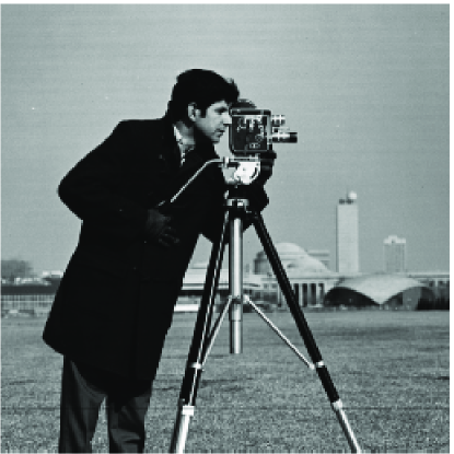
(a) Cameraman ($256\times 256$).

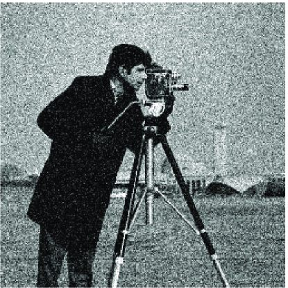
(b) Corrupted: $18.61$ dB ($\sigma=30$).

(c) SBF: $24.76$ dB; ($2,45$).

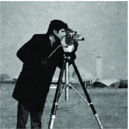
(d) WBF: $\bf{26.38}$ dB; ($4,20$).

Fig. 1: Denoising results using standard bilateral filter (SBF) and the proposed weighted bilateral filter (WBF). For reproducibility, we used the builtin Camerman image that comes with Matlab. We tuned the parameters of SBF and WBF to get the optimal PSNR in either case. The optimal ($\sigma_{s},\sigma_{r}$) setting is indicated in the caption.

6 Conclusion

We demonstrated how a simple pre-processing step can substantially improve the denoising performance of the bilateral filter. To consistently get the best of the standard and the pre-processed filter at all noise levels, we proposed to optimally weight them using Stein’s unbiased estimate of the MSE. The optimal weights were found by solving a small linear system. A fast algorithm for implementing the optimally-weighted filters was also described. We reported visual and PSNR results on test images which confirmed the improvement over the original bilateral filter. An interesting finding was that the weighted bilateral filter is competitive with the non-local means filter.

References

- [1] L. P. Yaroslavsky, Digital Picture Processing. Secaucus, NJ: Springer-Verlag, 1985.
- [2] L. I. Rudin, S. Osher, and E. Fatemi, “Nonlinear total variation based noise removal algorithms,” Physica D: Nonlinear Phenomena, vol. 60, no. 1, pp. 259-268, 1992.
- [3] R. R. Coifman and D. L. Donoho, Translation-invariant De-noising. Springer, New York, 1995.
- [4] P. Perona and J. Malik, “Scale-space and edge detection using anisotropic diffusion,” IEEE Transactions on Pattern Analysis and Machine Intelligence, vol. 12, no. 7, pp. 629-639, 1990.
- [5] J. Portilla, V. Strela, M. J. Wainwright, and E. P. Simoncelli, “Image denoising using scale mixtures of Gaussians in the wavelet domain,” IEEE Transactions on Image Processing, vol. 12, no. 11, pp. 1338-1351, 2003.
- [6] A. Buades, B. Coll, and J. M. Morel, “A non-local algorithm for image denoising,” Proc. IEEE Computer Vision and Pattern Recognition, vol. 2, pp. 60-65, 2005.
- [7] S. P. Awate and R. T. Whitaker, “Unsupervised, information-theoretic, adaptive image filtering for image restoration,” IEEE Transactions on Pattern Analysis and Machine Intelligence, vol. 28, no. 3, pp. 364-376, 2006.
- [8] C. Kervrann and J. Boulanger, “Optimal spatial adaptation for patch-based image denoising,” IEEE Transactions on Image Processing, vol. 15(10), 2866-2878, 2006.
- [9] M. Elad and M. Aharon, “Image denoising via sparse and redundant representations over learned dictionaries,” IEEE Transactions on Image Processing, vol. 15, no. 12, pp. 3736-3745, 2006.
- [10] K. Dabov, A. Foi, V. Katkovnik, and K. Egiazarian, “Image denoising by sparse 3-D transform-domain collaborative filtering,” IEEE Transactions on Image Processing, vol. 16, pp. 2080-2095, 2007.
- [11] T. Blu and F. Luisier, “The SURE-LET approach to image denoising,” IEEE Transactions on Image Processing, vol. 16, pp. 2778-2786, 2007.
- [12] P. Milanfar, “A tour of modern image filtering: new insights and methods, both practical and theoretical,” IEEE Signal Processing Magazine, vol. 30, no. 1, pp. 106-128, 2013.
- [13] C. Tomasi and R. Manduchi, “Bilateral filtering for gray and color images,” Proc. IEEE International Conference on Computer Vision, pp. 839-846, 1998.
- [14] M. Aleksic, M. Smirnov, and S. Goma, “Novel bilateral filter approach: Image noise reduction with sharpening,” Proc. Digital Photography II Conference, vol. 6069, SPIE, 2006.
- [15] C. Liu, W. T. Freeman, R. Szeliski, and S. Kang, “Noise estimation from a single image,” Proc. IEEE Computer Vision and Pattern Recognition, vol. 1, pp. 901-908, 2006.
- [16] P. Kornprobst and J. Tumblin, Bilateral Filtering: Theory and Applications. Now Publishers Inc., 2009.
- [17] C. Knaus and M. Zwicker, “Progressive Image Denoising,” IEEE Transactions on Image Processing, vol. 23, no.7, pp. 3114-3125, 2014.
- [18] N. Pierazzo, M. Lebrun, M. E. Rais, J. M. Morel, and G. Facciolo, “Non-local dual denoising,” Proc. IEEE International Conference on Image Processing, 2014.
- [19] C. Stein, “Estimation of the mean of a multivariate normal distribution,” Annals of Statistics, vol. 9, pp. 1135-1151, 1981.
- [20] H. Peng and R. Rao, “Bilateral kernel parameter optimization by risk minimization,” Proc. IEEE International Conference on Image Processing, pp. 3293-3296, 2010.
- [21] H. Kishan and C. S. Seelamantula, “Sure-fast bilateral filters,” Proc. IEEE International Conference on Acoustics, Speech and Signal Processing, pp.1129-1132, 25-30, 2012.
- [22] K. N. Chaudhury, D. Sage, and M. Unser, “Fast bilateral filtering using trigonometric range kernels,” IEEE Transactions on Image Processing, vol. 20, no. 12, pp. 3376-3382, 2011.
- [23] K. N. Chaudhury, “Acceleration of the shiftable algorithm for bilateral filtering and nonlocal means,” IEEE Transactions on Image Processing, vol. 22, no. 4, pp. 1291-1300, 2013.
- [24] R. Deriche, “Recursively implementing the Gaussian and its derivatives,” Research Report INRIA-00074778, 1993.
- [25] K. N. Chaudhury, Robust Bilateral Filter (http://www.mathworks.com/matlabcentral/fileexchange/50855-robust-bilateral-filter), MATLAB Central File Exchange. Retrieved May 15, 2015.
- [26] The USC-SIPI Image Database, http://sipi.usc.edu/database/.