A numerical study of the
Regge Calculus and Smooth Lattice methods
on a Kasner cosmology.

Abstract

Two lattice based methods for numerical relativity, the Regge Calculus and the Smooth Lattice Relativity, will be compared with respect to accuracy and computational speed in a full 3+1 evolution of initial data representing a standard Kasner cosmology. It will be shown that both methods provide convergent approximations to the exact Kasner cosmology. It will also be shown that the Regge Calculus is of the order of 110 times slower than the Smooth Lattice method.

1 Introduction

This is a good time to be doing numerical relativity. Most of the important hard problems have largely been solved to the extent that computations with important astrophysical applications are now treated, to a degree, as routine. But past experience with computational physics indicates that new algorithms will be required and thus it seems timely to revisit alternative approaches to numerical relativity.

Lattice based methods, such as the Regge Calculus [1, 2], have most commonly been used as a possible basis for quantum gravity and, to a lesser extent, in numerical relativity. They provide an elegant distinction between the topological properties of the lattice (by way of the connections between the vertices) and the geometry of the lattice (by the assignment of lengths to the legs). The ease with which complex topologies can be encoded in a lattice is often cited as a clear advantage of lattice methods over traditional grid based methods (though this claim has yet to be demonstrated in a non-trivial example).

In this paper two lattice based methods, the Regge Calculus [1, 2, 3] and Smooth Lattice Relativity [4, 5, 6] will be compared head to head with particular emphasis on the computational costs and to a lesser extent the accuracy of both methods for a simple $T^{3}$ Kasner cosmology. Our results show (see section (6)) that both methods provide convergent approximations to the continuum but at vastly different computational cost – the Regge Calculus is around 110 times slower than the smooth lattice method. This is a severe limitation that precludes meaningful comparison of the two methods for less symmetric space-times. Comparisons of the Smooth Lattice Method with traditional finite difference methods for the Teukolsky, Brill and Gowdy space-times will be presented elsewhere.

2 Smooth Lattice Relativity

Since the smooth lattice method is not well known it is reasonable to take a short moment to describe its basic features.

Put simply, the smooth lattice is a discrete approximation to some possibly unknown smooth geometry. In the case where the smooth geometry is known explicitly it is rather easy to construct a discrete approximation, the smooth lattice, from the given smooth geometry. The smooth geometry is required only to provide the necessary information, its topology and metric, to allow the construction to proceed. It serves no real purpose after the construction of the lattice (though it might reappear when questions of convergence are addressed).

Consider some given smooth geometry composed of a smooth manifold equipped with a smooth metric. How might a discrete approximation to that geometry be built? The short answer is that the manifold can be approximated by a finite lattice and the metric by an assignment of lengths to the legs of the lattice. But how is that lattice constructed? And how is the assignment of leg lengths made?

The lattice can be built by drawing upon familiar ideas from differential geometry. Recall that an atlas on a manifold consists of a sequence of overlapping charts and transition functions between pairs of neighbouring charts. Given any atlas, a lattice can be constructed simply by introducing one vertex per chart and connecting each vertex to its nearest neighbours (these connections will be the legs of the lattice). Other choices are of course possible (e.g., by adding more vertices in each chart) but this serves as a simple example. Now consider the metric and its encoding on the lattice. It is tempting to declare that each leg of the lattice is also a geodesic segment of the continuum geometry. But doing so introduces a minor problem – there may exist legs in the lattice which fail to be described by a unique geodesic. Fortunately this is easily fixed by simply refining the charts into smaller and smaller charts to the point that every leg in the lattice is described by a unique geodesic. It is well known that it is always possible to do so (in the absence of curvature singularities).

The final step in this construction is to adopt local Riemann normal coordinates in a neighbourhood of a selected vertex. This is done for a number of reasons

• it captures the essence of the Einstein equivalence principle,

• it guarantees that, in the absence of space-time singularities, the Riemann components are bounded,

• it reduces covariant derivatives to partial derivatives and a consequent reduction in the complexity of many differential operators.

In the local Riemann normal coordinates, $x^{\mu}=(t,x,y,z)^{\mu}$, the metric can be written as

$$g_{\alpha\beta}(x) =g_{\alpha\beta}-\frac{1}{3}R_{\alpha\mu\beta\nu}x^{\mu}x^{\nu}+\frac{1}{12}R_{\alpha\mu\beta\nu,\gamma}x^{\mu}x^{\nu}x^{\gamma}+\mathcal{O}\left(L^{4}\right)$$ (2.1)

where $L$ is a typical length scale for the neighbourhood of the vertex and $g_{\alpha\beta}={\rm diag}(-1,1,1,1)$. This choice of $g_{\alpha\beta}$ ensures that the coordinate basis vectors $\partial_{a}$ form an orthonormal basis for the tangent space at the chosen vertex.

It is a straightforward computation to show, given the above form of the metric, that the length $L_{ij}$ of the geodesic segment connecting vertices $i$ and $j$ is given by [7, 8]

$$L_{ij}^{2} =g_{\alpha\beta}\Delta x^{\alpha}_{ij}\Delta x^{\beta}_{ij}-\frac{1}{3}R_{\alpha\mu\beta\nu}x^{\alpha}_{i}x^{\beta}_{j}x^{\mu}_{i}x^{\nu}_{j}+\mathcal{O}\left(L^{5}\right)$$ (2.2)

These equations can be used to compute the coordinates of each vertex $x^{\alpha}_{i}$ given the $L_{ij}$ and $R_{\alpha\beta\mu\nu}$ as described in section (6) of [5]. The translational and rotational symmetries are accounted for by locating the coordinate origin at the chosen vertex while aligning selected coordinate axes with specific legs of the lattice.

The construction just given will produce a smooth lattice that is discrete in both space and time. However, it is standard practice in numerical relativity to cast the Einstein equations in the form of a Cauchy initial value problem. This imposes a small change in the process described above. Prior to introducing the lattice, the smooth 4 dimensional space-time is assumed to be foliated into a sequence of Cauchy surfaces. A 3 dimensional lattice is built from a set of vertices in an initial Cauchy surface and subsequently propagated onto future Cauchy surfaces by the Einstein equations and suitable gauge conditions. In this picture the leg lengths, Riemann curvatures and coordinates are now regarded as functions of time. Importantly the legs and the Riemann curvatures retain their 4 dimensional status (i.e., each leg is a geodesic of the 4-dimensional metric not the 3-metric of the Cauchy surface, each leg is a chord of the space-time connecting pairs of vertices in the Cauchy surface). This is perhaps not obvious at this point but will be made clear later after introducing the full set of evolution equations.

In making the transition from concepts based in differential geometry to a discrete lattice it helps to introduce some new terminology and notation (to emphasise the distinction between continuum and discrete structures). Thus a neighbourhood of a selected vertex will be known as a cell on a central vertex. The cell will consist of its central vertex together with its immediate neighbouring vertices and the set of legs shared by those vertices. A frame will be defined as a cell together with a set of geometrical data for that cell including (no less than) a local set of coordinates, the leg lengths for each leg in the cell and the Riemann curvatures at the central vertex.

Cells will overlap and this requires some care when specifying frame dependent quantities (such as tensor components). The following notation will be introduced to avoid any ambiguity. A quantity $R$, defined on vertex $q$ in the frame of vertex $p$, will be denoted by $R_{q\overline{p}}$. The subscripts $q\overline{p}$ will be dropped in cases where no ambiguity can arise.

Vertices in a cell will be denoted by lowercase Latin letters while Greek letters will be used for all tensor indices.

2.1 The SLGR evolution equations

In an earlier paper [5] a set of evolution equations for the lattice were proposed in which the dynamical variables were the leg lengths, their first time derivatives and the Riemann curvatures. The extrinsic curvatures and vertex coordinates were treated as kinematical variables and were computed as solutions of simple algebraic equations (see sections (6.1) and (7.1) of [5]). The experience gained since then shows that there are better choices for the dynamical variables leading to greatly simplified evolution equations and considerably reduced computational cost. Two choices for the dynamical variables will be presented. The first uses $(L_{ij},K_{\alpha\beta},R_{\alpha\beta\mu\nu})$ as dynamical variables while the second uses $(x^{\mu}_{i},K_{\alpha\beta},R_{\alpha\beta\mu\nu})$. In both cases equations (2.2) are used to compute the remaining data, either $x^{\mu}_{i}$ or $L_{ij}$, from the dynamical variables.

In the case of a unit lapse and zero shift vector, as used throughout this paper, the evolution equations for the leg lengths and extrinsic curvatures (see equations (3.1,3.2) of [5]) are

$$\frac{dL_{ij}^{2}}{dt} =-2K_{\alpha\beta}\Delta x^{\alpha}_{ij}\Delta x^{\beta}_{ij}$$ (2.3)

$$\frac{d}{dt}\left(K_{\alpha\beta}\Delta x^{\alpha}_{ij}\Delta x^{\beta}_{ij}\right) =\left(-K_{\mu\alpha}K^{\mu}{}_{\beta}+R_{\alpha t\beta t}\right)\Delta x^{\alpha}_{ij}\Delta x^{\beta}_{ij}$$ (2.4)

where $\Delta x^{\alpha}_{ij}=x^{\alpha}_{i}-x^{\alpha}_{j}$, $R_{\mu t\nu t}=R_{\mu\alpha\nu\beta}n^{\alpha}n^{\beta}$ and $n^{\mu}=\delta^{\mu}{}_{t}$ is the future pointing unit time-like normal to the Cauchy surface at the central vertex.

The normal use of equations (2.3,2.4) would be to dictate the evolution of legs in the lattice. There is, however, no reason why that pair of equations can not be applied to any leg whether or not it happens to be defined by a pair of vertices of the lattice. This simple observation can be put to good use to obtain explicit evolution equations for each of the extrinsic curvatures. As an example, consider a fictitious leg defined by the coordinates $(0,0,0,0)$ and $(0,L_{xx},0,0)$. When substituted into (2.3,2.4) this leads to the following pair of evolution equations

$$\frac{dL_{xx}^{2}}{dt} =-2K_{xx}L_{xx}^{2}$$ (2.5)

$$\frac{d}{dt}\left(K_{xx}L_{xx}^{2}\right) =-K_{x\alpha}K^{\alpha}{}_{x}L_{xx}^{2}+R_{txtx}L_{xx}^{2}$$ (2.6)

which, upon eliminating $L_{xx}$, leads to

$$\frac{dK_{xx}}{dt}=K_{xx}^{2}-K_{xy}^{2}-K_{xz}^{2}+R_{txtx}$$ (2.7)

This same idea can be employed for the remaining extrinsic curvatures with the result that

$$\frac{dK_{yy}}{dt} =K_{yy}^{2}-K_{xy}^{2}-K_{yz}^{2}+R_{tyty}$$ (2.8)

$$\frac{dK_{zz}}{dt} =K_{zz}^{2}-K_{xz}^{2}-K_{yz}^{2}+R_{tztz}$$ (2.9)

$$\frac{dK_{xy}}{dt} =-K_{xz}K_{yz}+R_{txty}$$ (2.10)

$$\frac{dK_{xz}}{dt} =-K_{xy}K_{yz}+R_{txtz}$$ (2.11)

$$\frac{dK_{yz}}{dt} =-K_{xy}K_{xz}+R_{tytz}$$ (2.12)

(for the mixed terms such as $dK_{xy}/dt$, use a fictitious leg joining $(0,0,0,0)$ and $(0,L_{xx},L_{yy},0)$).

The evolution equations for the coordinates can be obtained by basic arguments (see Appendix Evolution of the RNC’s for full details). The result, for the vertex $q$ in the frame of $\overline{p}$, is

$$\frac{dx^{\mu}_{q\bar{p}}}{dt}=-K^{\mu}{}_{\nu}x^{\nu}_{q\bar{p}}+\mathcal{O}\left(L^{2}\right)\qquad\hbox{for }\mu=x,y,z$$ (2.13)

The final set of evolution equations for the lattice are those for the Riemann curvatures. These can be obtained from equations (4.4) to (4.17) of [5] which, in the simple case of a unit lapse function, are given by

$$\frac{dR_{xyxy}}{dt} =\phantom{+}R_{tyxy,x}-R_{txxy,y} \frac{dR_{xyxz}}{dt} =\phantom{+}R_{tzxy,x}-R_{txxy,z}$$ (2.14)

$$\frac{dR_{xyyz}}{dt} =\phantom{+}R_{tzxy,y}-R_{tyxy,z} \frac{dR_{xzxz}}{dt} =\phantom{+}R_{tzxz,x}-R_{txxz,z}$$ (2.15)

$$\frac{dR_{xzyz}}{dt} =\phantom{+}R_{tzxz,y}-R_{tyxz,z} \frac{dR_{yzyz}}{dt} =\phantom{+}R_{tzyz,y}-R_{tyyz,z}$$ (2.16)

$$\frac{dR_{txxy}}{dt} =-R_{xyxy,y}-R_{xyxz,z} \frac{dR_{tyxy}}{dt} =\phantom{+}R_{xyxy,x}-R_{xyyz,z}$$ (2.17)

$$\frac{dR_{tzxy}}{dt} =\phantom{+}R_{xyxz,x}+R_{xyyz,y} \frac{dR_{txxz}}{dt} =-R_{xyxz,y}-R_{xzxz,z}$$ (2.18)

$$\frac{dR_{tyxz}}{dt} =\phantom{+}R_{xyxz,x}-R_{xzyz,z} \frac{dR_{tzxz}}{dt} =\phantom{+}R_{xzxz,x}+R_{xzyz,y}$$ (2.19)

$$\frac{dR_{tyyz}}{dt} =\phantom{+}R_{xyyz,x}-R_{yzyz,z} \frac{dR_{tzyz}}{dt} =\phantom{+}R_{xzyz,x}+R_{yzyz,y}$$ (2.20)

The above equations (2.14–2.20) are nothing more than the second Bianchi identities coupled with the vacuum Einstein equations. The use of partial derivatives rather than covariant derivatives stems from the use of Riemann normal coordinates (in which the connection vanishes).

In summary, the evolution equations for the first set of dynamical variables $(L_{ij},K_{\alpha\beta},R_{\alpha\beta\mu\nu})$ are (2.3,2.7–2.12) and (2.14–2.20) while for the second set of dynamical variables, $(x^{\mu}_{i},K_{\alpha\beta},R_{\alpha\beta\mu\nu})$, the evolution equations are (2.13,2.7–2.12) and (2.14–2.20).

In the following these two sets of evolution equations will be referred to as evolution schemes 1 and 2 respectively.

2.2 The SLGR source terms

Given that the Riemann curvature components are known at each vertex of the lattice it would seem that the source terms in (2.14–2.20) could be easily evaluated using a suitable finite difference scheme. There is however one important issue that must be noted. In any cell the point values of the Riemann curvatures are known only at the central vertex. The values on the remaining vertices are with respect to the local frames associated with neighbouring cells. Thus before the finite differences are taken, the curvatures must first be imported, from the neighbouring frames, into the frame of the chosen cell. Fortunately this is rather straightforward task. The key observation is that a pair of neighbouring cells will share a set of legs. Choose one of the vertices and pick four of the shared legs attached to that vertex. To each leg construct a tangent vector and its corresponding components with respect to each frame. Assuming that this set of vectors are linearly independent (it will argued later in section (The SLGR source terms) that this assumption will almost always be satisfied) then there exists a unique map between the two frames (at this vertex). This map between the frames is the discrete analog of the transition functions from the continuum. It is this map that is used when importing data from one frame to another. See section (The bi-cubic lattice) for full details on how this map can be computed for the bi-cubic lattice.

For any chosen cell this procedure will produce, at each vertex of the cell, the components of the Riemann curvature in the frame of that cell. This data can then be used to estimate the partial derivatives at the central vertex. Note that the data will, in general, not lie on a regular grid thus the best that can be hoped for is for first order accurate estimates in the derivatives (i.e., an $\mathcal{O}\left(L\right)$ truncation error). This is not ideal but is the best that can be obtained with nearest neighbour interactions.

3 The Regge calculus

The Regge Calculus and the Smooth Lattice method are built on a common structure – they both use a lattice and a table of leg lengths in forming a discrete approximation to a continuum geometry. The principal difference between the two approaches lies in the nature of the metric assigned to the lattice. The Regge calculus requires that the metric be piecewise flat while the Smooth Lattice methods uses a locally flat approximation. The curvature in a piecewise flat metric must be treated as a distribution with support on the two dimensional subspaces of the lattice (commonly known as bones or hinges and are usually the triangular faces of the 4-simplices of the lattice; the 4-simplex is the canonical cell in a Regge lattice). Working with distribution valued quantities in a non-linear theory such as General Relativity is a mathematically delicate area and requires considerably care. The upshot is that the Einstein equations can not be easily imposed onto the Regge lattice. However it is possible [9] to unambiguously evaluate the Hilbert action on a Regge lattice, leading to

$$I=\sum_{M}\>\theta A$$ (3.1)

where the sum includes all of the bones within the lattice $M$ and $\theta$ and $A$ are the defect angle and area of a typical bone (both of which can be computed from the known leg lengths). Then, in analogy with the continuum case, the evolution equations for the lattice, the Regge equations, are normally obtained by extremising this action with respect to the leg lengths. Extremising with respect to leg $L_{ij}$ leads to

$$0=\sum_{M(L_{ij})}\>\theta\frac{\partial A}{\partial L_{ij}}$$ (3.2)

where the sum now includes just the bones attached to the leg. There is one such equation for each leg of the lattice. See [1] for full details.

3.1 The Regge evolution equations

The equations just given are the full set of evolution equations for the Regge Calculus. Though the equations are elegant they do present three hurdles. The first is one of computational complexity – the defects as functions of the legs are so involved that it is simply not possible to present explicit expressions for the defects in terms of the leg lengths (though the full details of the algorithm can be found in [10]). The second hurdle concerns the way in which the Regge equations are solved – they are a fully coupled non-linear set of algebraic equations for the 4-dimensional leg lengths. Gentle and Miller [11] employ a Sorkin evolution scheme [12, 13] in which a pair of existing Cauchy surface are used to push forward to a future Cauchy surface. The Sorkin scheme provides a very elegant means of solving the Regge equations though it does require some careful bookkeeping. The final hurdle is more conceptual – how can account be taken of the freedom to choose the lapse and shift vector? This point is addressed in detail by Gentle and Miller [11] where they argue that as the continuum limit is approached the above Regge equations must reveal four degrees of freedom at each vertex and thus four equations at each vertex must become redundant (in the continuum limit). They identify the four equations and provide details of how those equations can be used as part of the evolution scheme (in effect these equations propagate the vertices of one Cauchy surface while the remaining Regge equations propagate the leg lengths). The Sorkin evolution scheme, as implemented in this paper, is identical to that used by Gentle and Miller but with two minor exceptions. Firstly, in this paper the continuum metric is used to set the initial data (the consequences that follow from this choice will be discussed later in section (6)). Secondly, where Gentle and Miller identify three pairs of equations for the shift equations while later discarding one equation in each pair the approach taken in this paper is to take the average of each pair.

4 Initial data

It was previously noted that topological and geometrical properties of a lattice can be cleanly separated. This allows the initial data to be constructed in a two stage process. First, choose a lattice with the required topology. Then add to that (raw) lattice the required geometric data such as leg-lengths and, for the smooth lattice method, the Riemann and extrinsic curvatures.

4.1 The lattice

Following Gentle and Miller [11], each Cauchy surface will be modelled by a bi-cubic lattice with opposite faces identified (as required by the $T^{3}$ topology). This lattice is well suited to this cosmology as it allows not only to create initial data that are manifestly homogenous but also to create a family of arbitrarily refined lattices (so that convergence properties can be easily studied). The local structure of the lattice is shown in figure (1).

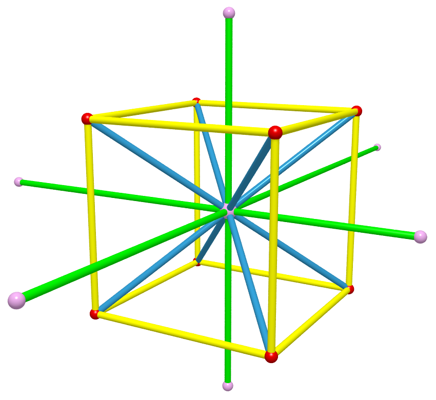
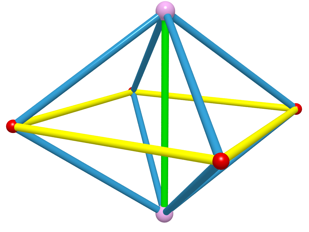
Figure 1: The local structure of the bi-cubic lattice. The lattice consists of two sub-lattices, one defined by the purple vertices, the other by the red vertices. These are the $A$ and $B$ lattices described in the text. The left figure displays the legs associated with one cell. The right figure shows the legs shared by a pair of cells.

There is one feature of this lattice that requires special mention. The set of cells can be split into two distinct groups. An element in one group is connected to another element in the same group by following legs aligned to the cube (e.g., a horizontal leg in figure (1)). While crossing from one group to the other requires moving along a diagonal leg. In principle this distinction could be ignored but in practice there is one advantage to be had. Denote the two groups by $A$ and $B$. The original lattice is the sum of this pair. It is possible to contemplate using the smooth lattice method on just group $A$ or on the pair $A$ and $B$. In each case the discretisation scale is the same but the later case would require twice the work (for no likely gain in accuracy). For this reason it was decided to apply the smooth lattice method to just one group (the choice is unimportant).

A little more work is needed for the Regge calculus as it requires a fully 4-dimensional lattice, bounded by two Cauchy surfaces and fully sub-divided into 4-simplices (a form of a thin-sandwich approach). This structure can be obtained by lifting, in stages, groups of vertices from one Cauchy surface forward in time to the second Cauchy surface. The full details can be found in [11].

4.2 Geometric data

Here a slightly different approach is taken compared to that taken by Gentle and Miller. They chose to set the initial data for their Regge lattice by solving the Regge initial data equations (a Regge form of the Hamiltonian and momentum constraints). This is a non-trivial task and requires the solution of a large system of non-linear algebraic equations. In this paper a much simpler approach was taken by setting the initial data for both the Regge calculus and the smooth lattice method directly from the exact form of the Kasner metric. It should be emphasised that this is not strictly correct (as the constraint equations are not necessarily satisfied) but as the computational cost of an evolution does not depend on how the initial data was set this short cut should have no impact on whatever conclusions might be drawn from the results (this point will be discussed further in section (7)).

The particular form of the vacuum Kasner $T^{3}$ cosmology used in this paper is described by

$$ds^{2}=-d{\bar{t}}^{2}+{\bar{t}}^{2a}d{\bar{x}}^{2}+{\bar{t}}^{2b}d{\bar{y}}^{2}+{\bar{t}}^{2c}d{\bar{z}}^{2}$$ (4.1)

where $a=b=4/3$ and $c=-1/3$. The non-standard notation for the coordinates $({\bar{t}},{\bar{x}},{\bar{y}},{\bar{z}})$ was chosen simply to avoid confusion with the local Riemann normal coordinates $(t,x,y,z)$ used in the smooth lattice equations. However, since both the local Riemann and global frames use a unit lapse and zero shift vector there should be no confusion in setting $t={\bar{t}}$.

Given the form of the Kasner metric (4.1) it is a simple matter to compute, for $t>0$, the various quantities employed in the lattice. The conversion to Riemann normal form (for the curvatures) is best done by projection onto a local orthonormal frame (i.e., onto the unit vectors parallel to the coordinate axes). This leads to

$$K_{xx}=-at^{-1}\>,\quad K_{yy}=-bt^{-1}\>,\quad K_{zz}=-ct^{-1}$$ (4.2)

$$R_{xyxy}=abt^{-2}\>,\quad R_{xzxz}=act^{-2}\>,\quad R_{yzyz}=bct^{-2}$$ (4.3)

The remaining components are either zero (e.g., $K_{xy}=0$) or can be obtained from the above using known symmetries (e.g., $R_{yxxy}=-R_{xyxy}$).

The initial 3 dimensional lattice was constructed as a cube of vertices evenly spaced in the Kasner $({\bar{t}},{\bar{x}},{\bar{y}},{\bar{z}})$ coordinates. Each vertex was assigned coordinates in the form $(a{\delta x},b{\delta y},c{\delta z})$ with $(a,b,c)$ a set of integers subject to $0\leq a\leq N_{x}$, $0\leq b\leq N_{y}$ and $0\leq c\leq N_{z}$. The integers $N_{x}$, $N_{y}$ and $N_{z}$ count the number vertices along the respective coordinate axes while the $({\delta x},{\delta y},{\delta z})$ are the coordinates increments between neighbouring vertices. The $T^{3}$ topology was obtained by identifying vertices on opposite faces of the cube, for example, by identifying $(0,b,c)$ with $(N_{x},b,c)$. This produces a cube of dimensions $(N_{x}{\delta x})\times(N_{y}{\delta y})\times(N_{z}{\delta z})$ in the Kasner coordinate space. The leg-lengths on this cube were set by solving the two-point boundary value problem for the geodesic equation while the Riemann and extrinsic curvatures were set using the exact data given by equations (4.2,4.3). All of the initial data were set at $t=1$.

The evolution of the initial data described in this paper uses a zero shift vector and a unit lapse. Thus the Kasner coordinates of a typical vertex will be of the form $(1+p{\delta t},a{\delta x},b{\delta y},c{\delta z})$ where $p$ is a positive integer and ${\delta t}$ is the time step between successive Cauchy surfaces. These coordinates will be used to compute exact values of the lattice data (leg-lengths, curvatures etc.) for comparison with the numerical evolutions.

5 Evolution

The Regge data was evolved following the method given by Gentle and Miller with the small exception previously noted (where the average of the pair of shift equations were taken rather than using just one equation). The smooth lattice equations were integrated using a 4th order Runge-Kutta scheme with a variable time step as described below (6).

For the smooth lattice method there remains one small issue – how can a unique time derivative be computed for legs that are shared by neighbouring cells? The simple answer is to take an average over all of the contributing cells. Note also in equation (2.3) the time derivative uses an off-centre estimate for the extrinsic curvature. This can be improved by constructing a linear Taylor series to estimate the $K_{\alpha\beta}$ at the centre of the leg with the first spatial derivatives of the $K_{\alpha\beta}$ computed in exactly the same manner as those for the $R_{\alpha\beta\mu\nu}$. Since the Kasner geometry is homogenous this step was not expected to make any significant changes to the evolution of the lattice.

6 Results

A number of simple tests were conducted to verify that both methods gave the expected results and to measure their rates of convergence to the continuum. In the first test the codes were run over $1<t<11$ with the initial data set at $t=1$ using $L=0.005$ while the evolutions used a variable time step ${\delta t}=\min(L_{xx},L_{yy},L_{zz})/4$. Convergence tests were performed by multiple integrations over $1<t<8$ each with successively smaller $L$ and corresponding ${\delta t}$. In particular, seven integrations were performed with a fixed time step ${\delta t}=L/5$ where $L=0.5/2^{q}$ and $q=1,2,3\cdots 7$. A fixed time step was chosen simply to make it easier to stop the evolution at exactly $t=8$.

There are three sets of data to be discussed, one for the Regge calculus and two for the smooth lattice method (one for each of the evolution schemes). For the moment the discussion will focus on the Regge calculus results versus those of the first evolution scheme for the smooth lattice method. The results for the second scheme will be presented at the end of this section.

On the $N_{x}=N_{y}=N_{z}=8$ lattice used by Gentle and Miller both the Regge calculus and smooth lattice methods produced extremely homogenous evolutions over $1<t<11$ with variations in $L_{xx}$ across the lattice of the order of the machine precision (which in this case was $10^{-18}$). Similar behaviour was noted in the extrinsic and Riemann curvatures in the smooth lattice results (no such data is readily available for the Regge calculus). The $N_{x}=N_{y}=N_{z}=8$ lattice is a rather coarse lattice so the calculations were repeated on a $N_{x}=512,N_{y}=N_{z}=8$ lattice with the results again being of the order of the machine precision.

The evolution of the fractional error in $L_{xx}$ and $L_{zz}$ are shown in figure (2). In this and following figures, the fractional error $E(Q)$ in some quantity $Q$ is defined by $E(Q)=1-Q/Q^{e}$ where the superscript $e$ denotes the exact value (as computed from the Kasner metric). There is little to note here other than that the errors are small and grow smoothly with time.

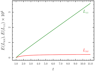
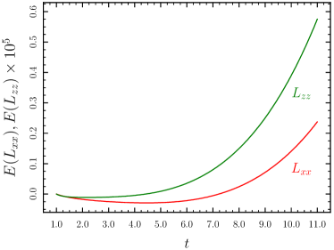
Figure 2: The fractional errors in the leg lengths for the Regge calculus (left) and the smooth lattice method (right).

The Hamiltonian constraint is shown in figure (3). The Regge Hamiltonian, as described in detail by Gentle and Miller, was scaled by an estimate of the volume per vertex $V=L_{xx}L_{yy}L_{zz}$ (in the spirit of Wheeler’s estimate of the 3-Riemann scalar ([3, 14])). The Smooth Lattice Hamiltonian is taken to be $H=2(R_{xyxy}+R_{xzxz}+R_{yzyz})$. This differs from the more familiar form of the Hamiltonian, namely $H={}^{(3)}R+K^{2}-K_{ab}K^{ab}$, for the simple fact that the smooth lattice method works directly with the 4-Riemann curvatures rather than the 3-Riemann curvatures. Figure (3) shows that the initial value of the Regge Hamiltonian is not zero. This is a direct consequence of setting the initial data via the exact solution rather than by enforcing the Regge constraints.

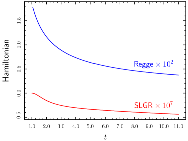
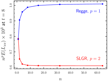
Figure 3: The Hamiltonian constraint (left) and the convergence estimate for the errors in $L_{xx}$ (right).

The convergence of the lattice solution to the continuum is displayed in the right hand panel of figure (3) and it would appear that while the smooth lattice method displays second order convergence the Regge calculus appears to be first order convergent. This conflicts with the second order convergence reported by Gentle and Miller. The most plausible explanation is that as the Regge initial data was not set by enforcing the Regge constraints, a first order error in the initial data has been introduced and that error has been propagated forward in time.

The smooth lattice method computes not just the leg-lengths but also the extrinsic and Riemann curvatures. These can be compared with the exact values (4.2,4.3). This leads to the results shown in figures (4) and (5). This again shows that the method tracks the exact solution very well. Plots such as these are not so easily constructed for the Regge calculus.

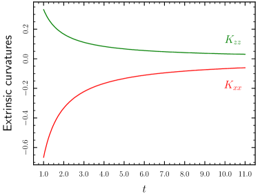
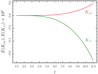
Figure 4: Smooth lattice evolution of $K_{xx}$ and $K_{yy}$ (left) and their corresponding fractional errors (right).

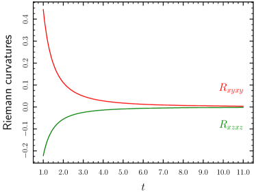
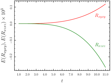
Figure 5: Smooth lattice evolution of $R_{xyxy}$ and $R_{xzxz}$ (left) and their corresponding fractional errors (right).

It should also be noted that where Gentle and Miller noticed high frequency oscillations in some of their data no such oscillations were observed in the Regge solutions described here. This difference is mostly likely due to the different ways in which the initial data were set.

The results presented above are all concerned with accuracy and convergence. But equally important is the computational cost. The $N_{x}=N_{y}=N_{z}=8$ models place very little demand on memory so the computational cost is dominated by the cpu time. It was found that the Regge calculus was around 110 times slower than the smooth lattice method. This poor performance is most likely due two keys elements of the Regge method – at each time step it has to solve 14 non-linear equations for 14 leg-lengths at each vertex while also frequently computing inverse trigonometric and hyperbolic functions. Despite using the best computational methods available [10] this gap between the Regge calculus and the smooth lattice method remained.

The results from the second evolution scheme for the smooth lattice were found to be significantly better than for the first scheme with a selection of results shown in figure (6). This scheme also runs much faster than the first scheme (it is quicker to evolve the coordinates than it is to solve the coupled quadratic equations (2.2)). In this case the smooth lattice method is approximately 170 times faster than the Regge calculus.

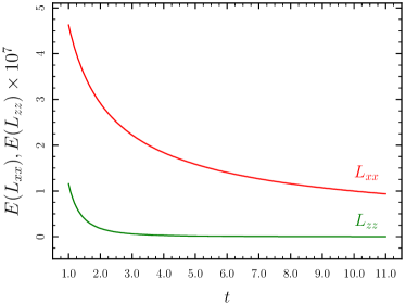
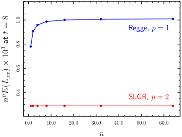
Figure 6: A sample of results for the second evolution scheme for the smooth lattice method. These results are a considerable improvement over the results from the first evolution scheme. The Hamiltonian is not plotted here as in this scheme it is zero throughout the evolution.

Given that this second scheme works so well the question must be – why bother with the first scheme? The simple answer is that the homogeneity of this space-time might be giving the second scheme advantages not shared with the first scheme. Another cause for concern with the second scheme is that it weakens the coupling between neighbouring frames. In the first scheme the evolution of the leg lengths was shared between pairs of frames (one from each vertex of the leg). In this second scheme the leg lengths are derived from the evolved coordinates of a single frame. It is not clear what impact this might have on the evolution of less symmetric initial data. Both schemes should be tested on space-times devoid of any symmetry before a decision is made on which is to be preferred.

7 Discussion

What objective conclusions can be drawn from the results just presented? Arguments may be made in favour of the formulation of both the Regge calculus and the smooth lattice method but such arguments are, to a degree, subjective being based on personal preferences. For example, the simplicity and elegance of the Regge calculus could be given as an argument in support of the Regge calculus. Equally, a case could be made that the smooth lattice method is better equipped to deal with differential operators on a lattice than the Regge calculus. But the real crunch comes when asking which method gives the better numerical results. That is, given the same initial data on the same lattice, how do the evolved data compare for accuracy, stability and cost in memory and cpu time? The question of accuracy can not be properly dealt with here for the simple reason that the initial data were not constructed as solutions of the respective constraint equations. However, as noted in section (4.2), the manner in which the initial data is constructed should have no bearing on the cpu time required to evolve the initial data. Thus the observation that the Regge calculus is 110 times slower (or worse) than the smooth lattice method must be taken seriously. If this number can not be reduced then it is hard to see how the Regge calculus could compete against the smooth lattice method. One approach might be to take advantage of the massive parallelism available in the Sorkin algorithm. However this is unlikely to do the trick as the same is true of the smooth lattice method. The questions of stability and memory are also of little value in this instance as both methods were seen to be stable over $1<t<11$ and required similar storage for these $8\times 8\times 8$ lattices. The upshot is that from the results presented above there is only one meaningful measure, the total cpu time, and that places the smooth lattice method well ahead of the Regge calculus.

The SLGR source terms

In section (2.2) it was noted that an essential step in estimating the sources terms, such as $R_{yzyz,y}$ in (2.20), requires data to be imported from one cell to another. The purpose of this section is to provide full details of that procedure. The following section will apply these ideas to the particular case of the bi-cubic lattice.

As a simple example, consider the case where the components of a vector $v^{\alpha}$, defined at vertex $q$, are to be imported from $\overline{q}$ to $\overline{p}$ (i.e., a transformation between frames). Since this map occurs in the tangent space of the vertex $q$ the transformation must be of the form

$$v^{\alpha}_{q\overline{p}} =M^{\alpha}{}_{\beta}(p,q)v^{\beta}_{q\overline{q}}$$ (.1)

for some yet to be determined $4\times 4$ matrix $M(p,q)$. The entries in $M(p,q)$ are not entirely arbitrary as the transformation must preserve scalar products (the transformation is simply a change of frame at a point). Thus the matrix $M$ is a proper Lorentz transformation characterised by six parameters – three boosts and three rotations.

So how might $M(p,q)$ be computed? If four linearly independent vectors at $q$ could be constructed, say $v^{\alpha}_{i},\>i=1,2,3,4$, and if their components in each frame could be found (by means other than from the above equation) then a system of equations such as

$$v^{\alpha}_{iq\overline{p}} =M^{\alpha}{}_{\beta}(p,q)v^{\beta}_{iq\overline{q}}\quad\quad i=1,2,3,4$$ (.2)

could be proposed for the unknown matrix $M(p,q)$. The assumption that the four vectors at $q$ are linearly independent ensures that a unique solution for $M(p,q)$ exists. This matrix can then be used to import data of any kind from $\overline{q}$ to $\overline{p}$, for example

$$K^{\alpha\beta}_{q\overline{p}}=M^{\alpha}{}_{\mu}(p,q)M^{\beta}{}_{\nu}(p,q)K^{\mu\nu}_{q\overline{q}}$$ (.3)

The challenge now is to first identify four linearly independent vectors $v^{\alpha}_{i},\>i=1,2,3,4$ and second their components in each frame. One of the vectors, $v^{\alpha}_{1}$, can be taken to be the future pointing time-like normal $n^{\alpha}$ to the Cauchy surface at $q$. But what of the remaining three vectors? This is where the legs of the lattice enters the picture – they provide the necessary information by which the vectors and their components can be constructed. Thus the remaining vectors, $v^{\alpha}_{i},\>i=2,3,4$, are chosen to be unit tangent vectors to three of the legs attached to $q$. There are of course many legs attached to $q$, so which three should be chosen? Since the unit vectors to these legs are about to be used to compute $M(p,q)$ it makes sense to choose legs that are shared by the cells $p$ and $q$. Now choose one of the three legs to be the leg joining $p$ to $q$. The remaining two legs can be freely chosen. This construction guarantees the linear independence of the four vectors at $q$ with one possible exception – when the last pair of legs just described coincide. This degenerate case is extremely unlikely to occur in practice and thus will be ignored.

The Riemann normal coordinates for any cell can be computed according to the procedure described in [5]. This in turn allows the tangent vectors to each leg to be computed at $q$ in each frame. In particular, the components of the unit tangent vector, at $q$, to the leg that joins $q$ to $r$ are given by

$$v^{\alpha}_{q\overline{q}}(q,r)L_{qr} =x^{\alpha}_{r\overline{q}}-x^{\alpha}_{q\overline{q}}$$ (.4)

$$v^{\alpha}_{q\overline{p}}(q,r)L_{qr} =x^{\alpha}_{r\overline{p}}-x^{\alpha}_{q\overline{p}}+\mathcal{O}\left(RL^{3}\right)$$ (.5)

where $x^{\alpha}$ are the Riemann normal coordinates. The first equation follows directly from the definition of Riemann normal coordinates while the second is the leading order expansion of the solution to the geodesic boundary value problem for the geodesic that connects $q$ to $r$. For full details see [7]. Note that although these vectors are tangent to the legs of the lattice they will not in general be orthogonal to the normal $n^{\alpha}$. This follows form the simple observation that the geodesic that joins a pair of vertices need not lie within the Cauchy surface but will in general be a chord for that pair of vertices. However, since the time coordinate of each vertex satisfies $2t=-K_{\alpha\beta}x^{\alpha}x^{\beta}$ (see [5]) it follows that $n^{\alpha}v_{\alpha}=\mathcal{O}\left(L^{2}\right)$.

Consider now the time-like vector normal $n^{\alpha}$. In the local Riemann normal coordinates with zero shift and unit lapse, the components for $n^{\alpha}$ in each frame are simply

$$n^{\alpha}_{p\overline{p}}=n^{\alpha}_{q\overline{q}}=\delta^{\alpha}_{t}$$

while the values for $n^{\alpha}_{q\overline{p}}$ can be estimated by a local Taylor series around $p$

$$n^{\alpha}_{q\overline{p}} =n^{\alpha}_{p\overline{p}}+n^{\alpha}{}_{;\beta}\Delta x^{\beta}(p,q)+\mathcal{O}\left(L^{2}\right)$$

However, for a unit lapse function,

$$n_{\mu;\nu}=-K_{\mu\nu}$$

where $K^{\alpha}{}_{\beta}$ are the components of the extrinsic curvature at $p$ in the frame $\overline{p}$. Thus the above equation can be re-written as

$$n^{\alpha}_{q\overline{p}}=\left(\delta^{\alpha}{}_{\beta}+n_{\beta}K^{\alpha}{}_{\gamma}x^{\gamma}_{q\overline{p}}\right)n^{\beta}_{q\overline{q}}+\mathcal{O}\left(L^{2}\right)$$ (.6)

This completes the construction of all four vectors in each frame and thus the transformation matrix $M^{\alpha}{}_{\beta}(p,q)$ can be computed from (.2).

The bi-cubic lattice

Consider for the moment the broad picture presented in section (2) in which a smooth lattice is constructed from a known smooth geometry $S$. Choose any set of coordinates over some subset $V$ of $S$. The intersection of the various coordinate planes in $V$ produces a set of cubic cells that can naturally be interpreted as the cells of a lattice. In this construction the unit vectors tangent to the legs of the cells will vary smoothly across the lattice. It is also clear, by increasing the density of the coordinate planes in $V$, that the unit vectors in one cell will converge to the corresponding unit vectors in a neighbouring cell. Thus the matrix $M(p,q)$ for a pair of cells, $p$ and $q$, not only reduces to the identity in the limit as $p$ approaches $q$ but it should do so smoothly. Consequently, for a bi-cubic lattice, $M(p,q)$ should be of the form

$$M^{\alpha}{}_{\beta}(p,q)=\delta^{\alpha}{}_{\beta}+m^{\alpha}{}_{\beta}(p,q)+\mathcal{O}\left(L^{2}\right)$$ (.1)

where $m(p,q)$ is another $4\times 4$ matrix at $q$ with entries $\mathcal{O}\left(L\right)$ and where $L$ is a typical length scale for the cell (e.g., the length of the leg joining $p$ to $q$).

Note that this result does not necessarily apply to other lattices, such as a simplicial lattice .

The matrix $m(q,p)$, like $M(p,q)$, is subject to the constraint that the transformations must preserve scalar products. Noting that the metric in each Riemann normal frame is of the form ${\rm diag}(-1,1,1,1)+\mathcal{O}\left(RL^{2}\right)$ it is easy to see that this leads to the following constraint on $m(p,q)$

$$0=g_{\alpha\rho}m^{\rho}{}_{\beta}(p,q)+g_{\beta\rho}m^{\rho}{}_{\alpha}(p,q)$$ (.2)

That is, the $m_{\mu\nu}$ define a skew-symmetric $4\times 4$ matrix determined by just six independent entries (corresponding to the three boosts and three rotations).

Note that equation (.6) is already in the form (.1) and thus it provides some immediate information about $m(p,q)$. It follows from (.1,.2) and (.6) that $m(p,q)$ is of the form

$$m^{\alpha}{}_{\beta}(p,q)=n_{\beta}K^{\alpha}{}_{\gamma}x^{\gamma}_{q\overline{p}}-n^{\alpha}K_{\beta\gamma}x^{\gamma}_{q\overline{p}}+s^{\alpha}{}_{\beta}(p,q)+\mathcal{O}\left(L^{2}\right)$$ (.3)

where $s(p,q)$ is another $4\times 4$ matrix subject to

$$0 =s^{\alpha}{}_{\beta}(p,q)n^{\beta}{}_{q\overline{q}}$$ (.4)

$$0 =s^{\alpha}{}_{\beta}(p,q)n_{\alpha q\overline{q}}$$ (.5)

(i.e., the matrix $s(p,q)$ has no normal component, it is a purely spatial matrix). In the adapted Riemann normal coordinates where $n^{\mu}=\delta^{\mu}_{t}$ and $g_{\mu\nu}={\rm diag}(-1,1,1,1)$ this requires the first row and column of $s(p,q)$ to be zero. Furthermore, the constraints (.2) shows that the remaining $3\times 3$ sub matrix of $s(p,q)$ must be skew symmetric. Thus $s(p,q)$ describes the three rotations while the remaining terms in $m(p,q)$ describe the three boosts.

The remaining entries in $s(p,q)$ can now be obtained by applying the transformation (.2) to the three vectors $v^{\mu}_{i},\>i=2,3,4$. This leads to a $3\times 3$ system for $s(p,q)$

$$v^{\alpha}_{iq\overline{p}}-v^{\alpha}_{iq\overline{q}}=s^{\alpha}{}_{\beta}(p,q)v^{\beta}_{iq\overline{q}}\quad\quad i=2,3,4$$ (.6)

where the Greek indices are now restricted to cover the $3\times 3$ sub-matrix of $s(p,q)$. This is an overdetermined system of equations for the three non-zero entries of $s^{\alpha}{}_{\beta}(p,q)$.

In appendix (The SLGR source terms) it was argued that the three vectors $v^{\mu}_{iq},\>i=2,3,4$ could be chosen as the unit vectors tangent to the legs at $q$. But equally any (invertible) linear combination of these vectors could also be used. This freedom can be used, as described below, to produce a near diagonal $3\times 3$ system of equations for $s(p,q)$.

The typical set of legs shared by a pair of cells in a bi-cubic lattice are shown in figure (7). This consists of five legs attached to $q$ and correspondingly, five tangent vectors $w^{\alpha}(i,q),\>i=p,a,b,c,d$. However the discussion above requires a selection of three linearly independent vectors at $q$. Many choices are possible, such as

$$v^{\alpha}_{2} =\lambda_{2}w^{\alpha}(p,q)$$ (.7)

$$v^{\alpha}_{3} =\lambda_{3}\left(w^{\alpha}(a,q)-w^{\alpha}(b,q)-w^{\alpha}(c,q)+w^{\alpha}(d,q)\right)$$ (.8)

$$v^{\alpha}_{4} =\lambda_{4}\left(w^{\alpha}(a,q)+w^{\alpha}(b,q)-w^{\alpha}(c,q)-w^{\alpha}(d,q)\right)$$ (.9)

with $\lambda_{i},\>i=2,3,4$ chosen so that each $v_{i},\>i=2,3,4$ is a unit vector. The justification for this choice is that, in the case of a flat lattice, the three vectors are aligned to the local coordinate axes. This is not an important point and many other choices might work equally as well. No such variations were tried for this paper. Note the change in notation – the $v_{i},\>i=2,3,4$ are not tangent to the legs, that role is now played by the $w(i,q),\>i=p,a,b,c,d$.

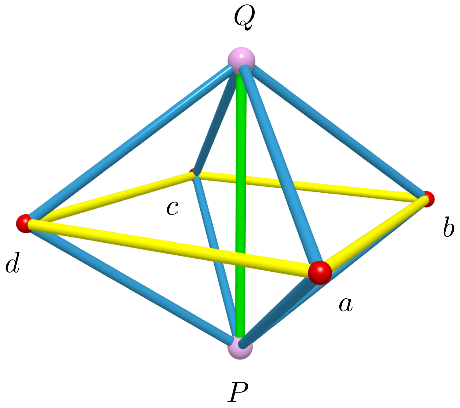
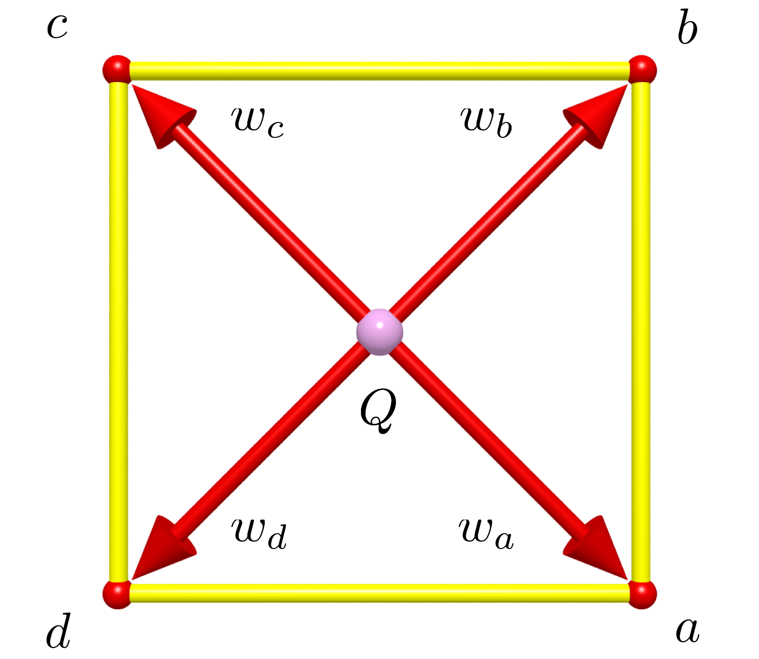
Figure 7: The set of legs shared by a pair of cells (left) and, viewed from above looking down on vertex $Q$, the set of vectors (right) used when constructing the map used to import the data from one frame to the other. Note that the labels $w_{a},w_{b}\cdots$ are abbreviations for the vectors $w(a,q),w(b,q)\cdots$ used in the text.

As noted above, the equations (.6) are an over determined system – they provide nine equations for just three non-zero entries in $s(p,q)$. The system could be solved using a least squares method but that is expensive (this calculation is at the heart of the evolution equations so computational cost is an important issue). The direct approach, as adopted in this paper, is to select just three of the nine equations and solve the resulting $3\times 3$ system using standard matrix methods. This worked very well for this lattice and this space-time. How were the three equations chosen? Consider for example the case were the lattice is almost flat. Then as noted above the three vectors $v^{\alpha}_{i},\>i=2,3,4$ will be closely aligned to the coordinate axes. Thus suppose $v_{2}$ is approximately aligned to the $x$-axis, $v_{3}$ to the $y$-axis and $v_{4}$ to the $z$-axis. Thus $v^{x}_{2}\approx 1,\>v^{y}_{3}\approx 1,\>v^{z}_{4}\approx 1$ while the remaining components have $|v^{\alpha}_{i}|=\mathcal{O}\left(L\right)$. Put

$$s(p,q)=\begin{bmatrix}0&{S_{xy}}&{S_{xz}}\\ -{S_{xy}}&0&{S_{yz}}\\ -{S_{xz}}&-{S_{yz}}&0\end{bmatrix}$$ (.10)

and then select the following three of the nine equations (.6)

$$\begin{bmatrix}v^{y}_{2q\overline{p}}-v^{y}_{2q\overline{q}}\\[3.0pt] v^{x}_{4q\overline{p}}-v^{x}_{4q\overline{q}}\\[3.0pt] v^{z}_{3q\overline{p}}-v^{z}_{3q\overline{q}}\end{bmatrix} =\begin{bmatrix}-v^{x}_{2q\overline{q}}&0&v^{z}_{2q\overline{q}}\\[3.0pt] v^{y}_{4q\overline{q}}&v^{z}_{4q\overline{q}}&0\\[3.0pt] 0&-v^{x}_{3q\overline{q}}&-v^{y}_{3q\overline{q}}\end{bmatrix}\begin{bmatrix}{S_{xy}}\\[3.0pt] {S_{xz}}\\[3.0pt] {S_{yz}}\end{bmatrix}$$ (.11)

By inspection it is easy to see that the diagonal entries of the coefficient matrix are close to $\pm 1$ while the remaining entries are small. Thus this $3\times 3$ equation is non-singular and easily solved for ${S_{xy}},{S_{xz}}$ and ${S_{yz}}$.

Even though the above equations (.11) were selected on the assumption that the lattice was almost flat they can be expected, on continuity arguments, to be useable in cases where the lattice is not approximately flat. This is consistent with the results in section (6) – at no point in the evolution did the $3\times 3$ set of equations have a condition number not close to one.

Once the matrices $m(p,q)$ are known for each of the vertices $q$ that surround $p$ then the derivatives of any tensor can be estimated at $p$ using a finite difference method. Consider the simple case where the spatial derivatives $u^{\mu}_{,x}$, $u^{\mu}_{,y}$ and $u^{\mu}_{,z}$ of some vector $u^{\mu}$ are required at $p$. Begin by writing out a short Taylor series

$$u^{\mu}_{q\overline{p}}=u^{\mu}_{p\overline{p}}+u^{\mu}_{,\nu p\overline{p}}x^{\nu}_{q\overline{p}}+\mathcal{O}\left(L^{2}\right)$$ (.12)

then use equations (.1) and (.1) to obtain

$$u^{\mu}_{,\nu p\overline{p}}x^{\nu}_{q\overline{p}}=u^{\mu}_{q\overline{q}}-u^{\mu}_{p\overline{p}}+m^{\mu}{}_{\alpha}(p,q)u^{\alpha}_{q\overline{q}}$$ (.13)

Note that the time coordinate $x^{t}_{q}=\mathcal{O}\left(L^{2}\right)$ and thus the left hand side only contains the three spatial derivatives. This system of equations can be written down, to $\mathcal{O}\left(L\right)$, for each of the vertices $q$ and once again leads to an overdetermined system for the spatial derivatives. For the bi-cubic lattice there is a rather simple reduction to a well defined $3\times 3$ system of equations. Define $\Delta u^{\mu}(p,q)$ by

$$\Delta u^{\mu}(p,q)=u^{\mu}_{q\overline{q}}-u^{\mu}_{p\overline{p}}+m^{\mu}{}_{\alpha}(p,q)u^{\alpha}_{q\overline{q}}$$ (.14)

Then build the following set of equations

$$u^{\mu}_{,\nu p\overline{p}}\left(x^{\nu}_{10}-x^{\nu}_{12}\right) =\Delta u^{\mu}(0,10)-\Delta u^{\mu}(0,12)$$ (.15)

$$u^{\mu}_{,\nu p\overline{p}}\left(x^{\nu}_{11}-x^{\nu}_{9}\right) =\Delta u^{\mu}(0,11)-\Delta u^{\mu}(0,9)$$ (.16)

$$u^{\mu}_{,\nu p\overline{p}}\left(x^{\nu}_{13}-x^{\nu}_{14}\right) =\Delta u^{\mu}(0,13)-\Delta u^{\mu}(0,14)$$ (.17)

in which the integers 10,12, etc. are the vertex labels (see figure (8)). This provides, for each choice of $\mu$, a $3\times 3$ system of equations for $u^{\mu}_{,\nu p\overline{p}}$. The same ideas can be used to compute the $R_{xyxy,z}$ etc.

Coordinates in the bi-cubic cell

In [5] a general procedure was given for computing the coordinates $x^{\mu}_{i}$ for each vertex in a cell. For the bi-cubic lattice the particular details are as follows.

The fifteen vertices of the cell are numbered for 0 to 14 as per figure (8). Consider three vertices $i$, $j$ and $k$ that form a tetrahedron attached to the central vertex. Suppose also that the coordinates for vertices $i$ and $j$ have been computed. Then the coordinates $x^{\mu}_{k}$ for vertex $k$ can be computed using

$$x^{\mu}_{k}=Px^{\mu}_{i}+Qx^{\mu}_{j}+Rn^{\mu}_{ij}$$

where

$$P=\frac{m_{ik}L^{2}_{oj}-m_{jk}m_{ij}}{L^{2}_{n}}\qquad Q=\frac{m_{jk}L^{2}_{oi}-m_{ik}m_{ij}}{L^{2}_{n}}$$

$$R=\frac{\left(L^{2}_{ok}-P^{2}L^{2}_{oi}-Q^{2}L^{2}_{oj}-2PQm_{ij}\right)^{1/2}}{L_{n}}$$

$$n^{\mu}_{ij}=g^{\mu\nu}\epsilon^{xyz}_{\nu\alpha\beta}x^{\alpha}_{i}x^{\beta}_{j}\qquad L^{2}_{n}=L^{2}_{oi}L^{2}_{oj}-m^{2}_{ij}$$

and where the $m_{ab}$ are defined by

$$2m_{ij}=L^{2}_{oi}+L^{2}_{oj}-L^{2}_{ij}$$

$$2m_{ik}=L^{2}_{oi}+L^{2}_{ok}-L^{2}_{ik}\quad\quad\quad 2m_{jk}=L^{2}_{oj}+L^{2}_{ok}-L^{2}_{jk}$$

Note the $n^{\mu}_{ij}$ is a vector normal to the triangle $(oij)$ pointing towards vertex $k$ (this can always be achieved by swapping $i$ and $j$ if required).

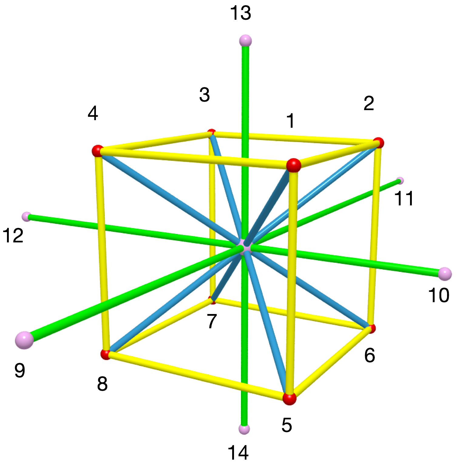
Figure 8: The bi-cubic cell with labels assigned to each vertex. The label for the central vertex is 0 but is excluded from this figure to avoid clutter. The local Riemann normal coordinates $(x,y,z)$ are chosen so that vertex 0 has coordinates $(0,0,0)$, vertex 13 lies on the positive $z$-axis and vertex 10 lies in the $xz$-plane with $x_{10}>0$.

The above procedure can be applied to all of the vertices provided initial values have been set for the first pair. This last step amounts to fixing the rotational freedoms. The frame chosen for this paper has the vertex 13 lying on the positive $z$-axis, i.e., $x_{13}=(0,0,x^{z}_{13})$ and vertex 10 lying somewhere in the $xz$-plane, i.e., $x_{10}=(x^{x}_{10},0,x^{z}_{10})$. However the cell does not contain the triangle $(0,10,13)$ and thus the coordinates for vertex 10, in this gauge, are not immediately available. This problem can be overcome by first choosing an intermediate gauge where vertex 1 lies in the $xz$-plane. In this gauge the coordinates for vertices 13 and 1 are easily computed,

$$x_{13}=(0,0,L_{0,13}),\qquad x_{1}=((L^{2}_{0,1}-m^{2}/L^{2}_{0,13})^{1/2},0,m/L_{0,13})$$ (.1)

with $m=(L^{2}_{0,1}+L^{2}_{0,13}-L^{2}_{1,13})/2$. This allows the coordinates for the remaining 13 vertices to be computed. Finally a rotation in the $xy$-plane is applied to cell to set $x^{y}_{10}=0$ and $x^{x}_{10}>0$.

Table (1) shows the order in which the vertex coordinates were computed (in the intermediate gauge). The notation $(k;i,j)$ indicates that the coordinates for vertex $k$ are computed form the known coordinates for vertices $i$ and $j$. Note that the order of $i$ and $j$ is important, they must be chosen so that the normal vector $n_{ij}$ points towards vertex $k$.

(2;13,1) (3;13,2) (4;13,3) (9;1,4) (10;,2,1) (11;3,2) (12;4,3) (5;1,9) (6;2,10) (7;3,11) (8;4,12) (14;6,5)

Table 1: The order in which the vertices are computed in the intermediate gauge. The entries should be read from left to right and top to bottom. Each entry is of the form (k;i,j) and this indicates that the coordinates of vertex $k$ are computed from the known coordinates of vertices $i$ and $j$. The coordinates of the central vertex are $(0,0,0)$ while the coordinates for vertices 13 and 1 are given by equation (.1).

Evolution of the RNC’s

In the standard Cauchy IVP there are two world-lines through any event, one is the observer’s world-line the other is the integral curve of the normal vector to the Cauchy surface containing that event. In a lattice method allowance must be made for a possible third world-line, the world-line of a vertex. Just as the observer’s world-line can be freely chosen in a given space-time so too can the vertex world-line. In the absence of any preferred spatial directions (e.g., the velocity vector of a fluid flow) a simple choice is to require each vertex to follow the integral curve of the normal vector and that in every cell the central vertex is forever located at the spatial origin (i.e., the shift vector vanishes at each central vertex). This is the choice made in this paper.

Let $x^{\mu}_{q\bar{p}}(t)$ be the coordinates along the world-line of vertex $q$ in the frame of $p$. Since this world-line coincides with the integral curve of the normal at $q$ it follows that the coordinates evolve according to

$$\frac{dx^{\mu}_{q\bar{p}}}{dt}=n^{\mu}_{q\bar{p}}$$ (.1)

which upon using (.6) and $n^{\mu}_{q\bar{q}}=\delta^{\mu}_{t}$ leads to

$$\frac{dx^{\mu}_{q\bar{p}}}{dt}=-K^{\mu}{}_{\nu}x^{\nu}_{q\bar{p}}+\mathcal{O}\left(L^{2}\right)\qquad\hbox{for }\mu=x,y,z$$ (.2)

These equations can be used to evolve the spatial part of the Riemann normal coordinates of each vertex within a cell. At any time the leg lengths can be recovered using (2.2).

References

- [1] T. Regge, General Relativity without coordinates, Il Nuovo Cimento XIX (1961) no. 3, 558–571.
- [2] A. P. Gentle, Regge calculus: a unique tool for numerical relativity, Gen. Rel. Grav. 34 (2002) 1701–1718, gr-qc/0408006.
- [3] J. A. Wheeler, Geometrodynamics and the Issue of the Final State, in Relativity, Groups and Topology, C. De Witt and B. De Witt, eds., pp. 467–500. Gordon and Breach Science Publishers, Inc., New York, 1964.
- [4] L. Brewin, An Einstein-Bianchi system for Smooth Lattice General Relativity. I. The Schwarzschild spacetime., Phys. Rev. D 85 (2012) no. 12, 124045, arXiv:1101.3171.
- [5] L. Brewin, An Einstein-Bianchi system for Smooth Lattice General Relativity. II. 3+1 vacuum spacetimes., Phys. Rev. D 85 (2012) no. 12, 124046, arXiv:1104.1356.
- [6] L. Brewin and J. Kajtar, A Smooth Lattice construction of the Oppenheimer-Snyder spacetime, Phys. Rev. D 80 (2009) 104004, arXiv:0903.5367. http://users.monash.edu.au/~leo/research/papers/files/lcb09-05.html.
- [7] L. Brewin, Riemann Normal Coordinate expansions using Cadabra, Class. Quantum Grav. 26 (2009) 175017, arXiv:0903.2087. http://users.monash.edu.au/~leo/research/papers/files/lcb09-03.html.
- [8] T. Willmore, Riemannian Geometry. Oxford University Press, Oxford, 1996.
- [9] J. Cheeger, W. Muller, and R. Schrader, On the curvature of piecewise flat spaces, Comm. Math. Phys. 92 (1984) 405–454.
- [10] L. Brewin, Fast algorithms for computing defects and their derivatives in the Regge calculus, Class. Quantum Grav. 28 (2011) 185005, arXiv:1011.1885. http://users.monash.edu.au/~leo/research/papers/files/lcb10-01.html.
- [11] A. P. Gentle and W. A. Miller, A fully (3 + 1)-dimensional Regge calculus model of the Kasner cosmology, Class. Quantum Grav. 15 (1998) 389–405.
- [12] R. Sorkin, Time-evolution problem in Regge calculus, Phys. Rev. D 12 (1975) 385–396.
- [13] J. W. Barrett, M. Galassi, W. A. Miller, R. D. Sorkin, P. A. Tuckey, and R. M. Williams, A parallelizable implicit evolution scheme for regge calculus, Int.J.Theor.Phys. 36 (1997) 815–840, arXiv:gr-qc/9411008v1.
- [14] T. Piran and R. M. Williams, Three-plus-one formulation of regge calculus, Phys. Rev. D 33 (1986) no. 6, 1622–1633.