Modeling neural activity at the ensemble level

Abstract

Here we demonstrate that the activity of neural ensembles can be quantitatively modeled. We first show that an ensemble dynamical model (EDM) accurately approximates the distribution of voltages and average firing rate per neuron of a population of simulated integrate-and-fire neurons. EDMs are high-dimensional nonlinear dynamical models. To faciliate the estimation of their parameters we present a dimensionality reduction method and study its performance with simulated data. We then introduce and evaluate a maximum-likelihood method to estimate connectivity parameters in networks of EDMS. Finally, we show that this model an methods accurately approximate the high-gamma power evoked by pure tones in the auditory cortex of rodents. Overall, this article demonstrates that quantitatively modeling brain activity at the ensemble level is indeed possible, and opens the way to understanding the computations performed by neural ensembles, which could revolutionarize our understanding of brain function.

1 Introduction

If we observe a fluid at the molecular level we see random motions, but if we look at it macroscopically we may see a smooth flow. An intriguing possibility is that by analyzing brain activity at a macroscopic level, i.e., at the level of neural ensembles, we may discover patterns not apparent at the single-neuron level, that are as useful as velocity or temperature are to understand, and predict, the motion of fluids.

Technology frequently drives science. For instance, thanks to the development of microelectordes in the 1930’s, we now know with exquiste detail computations performed by single neurons. We are now experiencing a dramatic increase in our capacity to monitor the activity of larger and larger populations of neurons with higher and higher spatial and temporal resolution. These new ensemble recordings may soon allow us to uncover crucial computations performed by neural ensembles.

Here we present results of developing and evaluating a mathematical model and estimation methods to characterize the activity of ensembles of neurons from electrophysiological data.

Section 2 reports the evaluation of an ensemble dyanmical model (EDMs). And EDMs is a high-dimensional nonlinear dynamical models. To estimate its parameters it is convenient to reduce the number of parameters. We escribe a dimensionality reduction method for EDMs in Section 3. Section 4 presents a maximum-likelihood method to estimate parameters of EDMs. Finally, in Section 5 we show that EDMs can accurately approximate high-gamma electroencephalographic activity evoked by pure tones in the auditory cortex of rodents.

2 Building EDMs

We wanted to learn how to build Ensemble Density Models (EDMs), dynamical models of the state variables (e.g., trans-membrane potential, time since last spike, etc.) of a population of identical neurons, starting from a dynamical model of the state variables of a single neuron. For Integrate and Fire (IF) model of single neurons, an EDM should provide the ensemble probability density function (pdf) $\rho(\upsilon,t)$, from which to compute the probability of finding a neuron in the ensemble with with a given trans-membrane voltage $\upsilon$ at time $t$ (i.e., $P(\upsilon,t)=\rho(\upsilon,t)dt$). It should also provide the average firing rate per neuron in the population, $r(t)$. To construct EDMs we chose the methodology described in Omurtag et al. (2000).

To evaluate the EDM we compared its outputs ($\rho(\upsilon,t)$ and $r(t)$) with those derived from the direct simulation of a population of 9,000 IF neurons. The value of the density function $\rho(\upsilon,t)$ derived from the direct simulation was the proportion of IF neurons having a voltage $\upsilon$ at time $t$, and the average firing rate per neuron $r(t)$ derived from the the direct simulation was the proportion of cells in the population at time $t$ with voltage at threshold.

An EDM is driven by an external excitatory current and modulated by an external inhibitory current. In addition, every cell in the EDM receives inputs from $G$ other neurons in the population. A fraction $f$ of these $G$ inputs is excitatory, and the remainder are inhibitory. These intra-population inputs act as feedback mechanisms to the EDM. The mathematical representation of an EDM for a population of IF neurons is given in Equations 1–3, modified from Equations 26, 39 and 47 in Omurtag et al. (2000). External excitatory and inhibitory currents appears as $\sigma^{0}_{e}(t)$ and $\sigma^{0}_{i}(t)$, respectively, in Equation 3, and excitatory and inhibitory feedback are given by the terms $Gfr(t)$ and $G(1-f)r(t)$, respectively, in Equation 3.

$$\frac{\partial\rho}{\partial t}(\upsilon,t) = -\frac{\partial J}{\partial\upsilon}(\upsilon,t)$$ (1)

$$r(t) = J(\upsilon=1,t)$$ (2)

$$J(\upsilon,t) = -\gamma\upsilon\rho(\upsilon,t)$$ (3)

$$+[\sigma^{0}_{e}(t)+Gfr(t)]\int_{\upsilon-h}^{\upsilon}\rho(\upsilon^{\prime},t)d\upsilon^{\prime}$$

$$-[\sigma^{0}_{i}(t)+G(1-f)r(t)]\int_{\upsilon}^{\upsilon/(1-\kappa)}\rho(\upsilon^{\prime},t)d\upsilon^{\prime}$$

We first verified that for a single population the outputs of the EDM matched those of the direct simulations (Section 2.1). We next built a network of excitatory and inhibitory populations, and again compared the outputs of the EDM and those of the direct stimulation (Section 2.2).

2.1 One Population

2.1.1 One Population of Independent Neurons

The top panel in Figure 1 shows the ensemble probability density function, $\rho(\upsilon,t)$, calculated by integrating the differential equation of an EDM, Equation 1. The bottom panel shows and approximation to this pdf obtained from the histogram of voltages of a direct simulation of a population of 9,000 IF neurons. Note the large similarity of the pdfs at all time points.

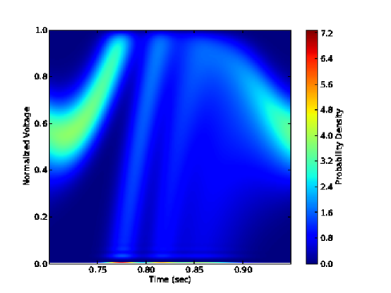
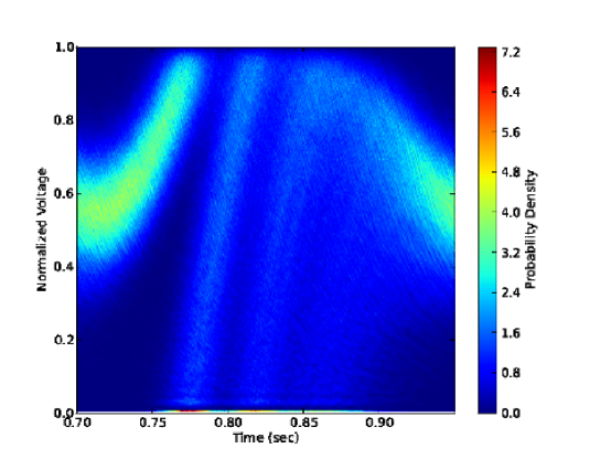
Figure 1: Ensemble pdf, $\rho(\upsilon,t)$, for a population of IF neurons in response to a sinusoidal input, calculated by integrating the differential equation of an EDM (Equation 1, top panel) and approximated by direct simulation of a population of 9,000 IF neurons (bottom panel). Neurons in this populations were independent of each other (i.e., they had no feedback; G=0 in Equation 3).

The black line in Figure 2 shows the average firing rate per neuron, $r(t)$, calculated using the EDM, Equation 2. The grey line shows the average firing rate per neuron calculated from a direct simulation of a population of 9,000 IF neurons, as the proportion of cells with voltage at threshold. Note the almost perfect match between these firing rates.

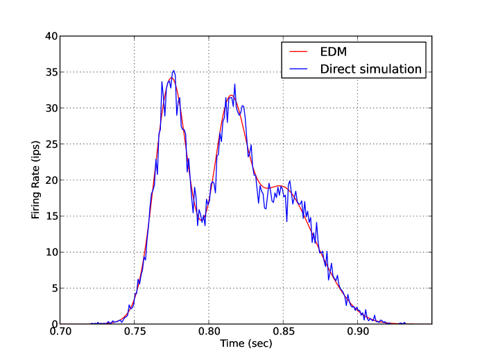
Figure 2: Firing rate of a population of neurons, in response to a sinusoidal input, calculated by direct simulation of a population of 9,000 IF neurons (grey line) and by integrating a population equation (black line, Equation 3). Neurons in this populations were independent of each other (i.e., they had no feedback; G=0 in Equation 3).

Figure 3 is as Figure 2 but for a step input current that jumps from 0 to 800 impulses per second at time $t=0$. Note that by 0.4 seconds after the step in the input current the average firing rate per neuron has reached a new steady state around 10 impulses per second, as revealed by the EDM (black line in Figure 3) and by the direct simulation of a population of 9,000 IF neurons (grey line, in Figure 3)). Figure 4 shows the pdf of voltages at this new steady state calculated by the EDM, Equation 2 (black line in Figure 4) and approximated using the histogram of voltages at 0.4 ms of a direct simulation of 9,000 IF neurons (grey line in Figure 4).

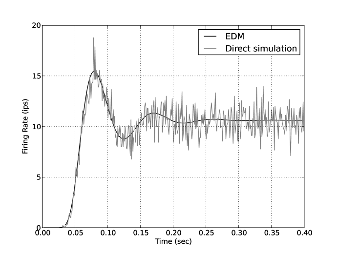
Figure 3: Firing rate of a population of 9,000 IF neurons, in response to a step input at time zero. Same format as in Figure 2

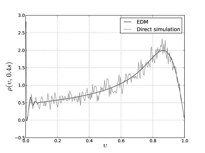
Figure 4: Ensemble pdf, $\rho(\upsilon,t)$ at 0.4 seconds in the neurons of the population of Figure 3 in response of a step input at time zero. This pdf was calculated by integrating the differential equation of an EDM (Equation 1, black line) and approximated using the histogram of the voltages of the simulated neurons (grey line).

2.1.2 One Population with Feedback

The previous Figures showed results from the simulation of a single population of independent neurons. Figure 5 is as Figure 2, but shows the average firing rate per neuron in a population where each neuron receives excitatory inputs from ten other neurons in the population (i.e., G=10 and f=1 in Equation 3). For comparison, the dashed line shows the average firing rate per neuron from the population without feedback.

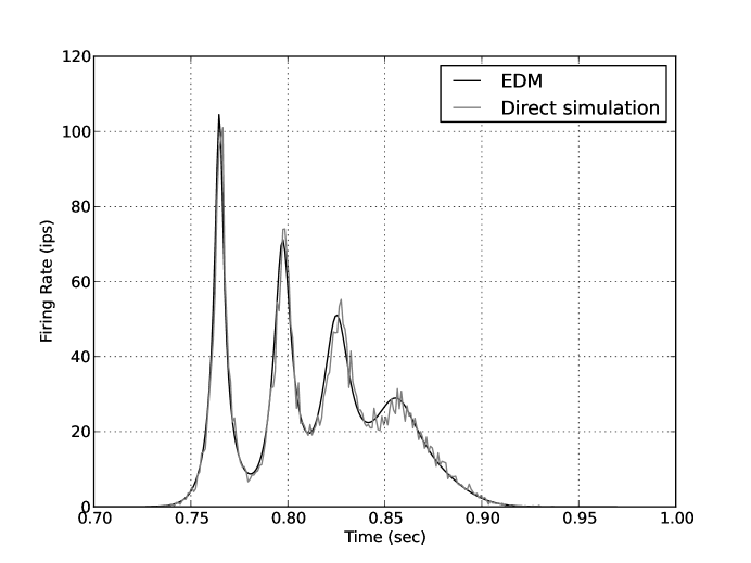
Figure 5: Firing rate of a population of 9,000 neurons, in response to a sinusoidal input, as in Figure 2, but each neuron in this population is connected with ten presynaptic neurons, and all of these neurons are excitatory (i.e., G=10 and f=1.0 in Equation 3).

Figure 6 demonstrates the effect of inhibitory feedback in the population of Figure 5 by changing the fraction of inhibitory input neurons from 0% to 80% (by changing f=1-0 to f=1-0.8, and still using G=10 in Equation 3).

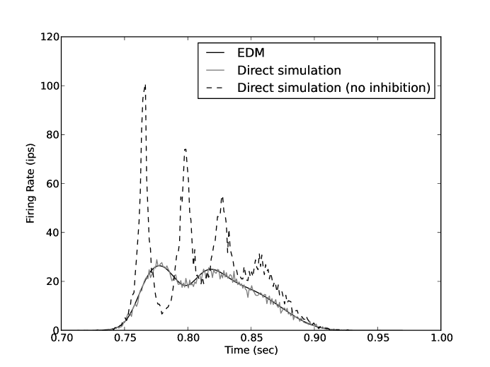
Figure 6: Same as Figure 5 but for a population of neurons where 80% of the presynaptic neurons to a given neuron are inhibitory (i.e., G=10 and f=1-0.8 in Equation 3). For comparison, the dashed line shows the average firing rate per neuron in the population with feedback but not inhibition of Figure 4.

2.2 A Network of Populations

The previous sections evaluated EDMs in a single population of neurons. Here we evaluate EDMs of excitatory and inhibitory populations combined in the network of populations shown in Figure 7. The network is driven by an excitatory input to the excitatory population. This population has excitatory feedback (i.e., G=5 and f=1 in Equation 3), and its average firing rate per neuron output, scaled by a constant $W_{ei}=50$, drives the inhibitory population. The inhibitory population has inhibitory feedback (i.e., G=5 and f=0 in Equation 3), and its average firing rate per neuron output , scaled by a constant $W_{ie}=15$, modulates the activity of the excitatory population.

Figure 7: Simulated network of two populations of IF neurons. A sinusoidal input, $\sigma^{0}(t)$, was applied to the excitatory population. This population contained excitatory feedback (each neuron in the population received excitatory input from five other neurons in the population; G=5, f=1 in Equation 3). The average firing rate per neuron of the excitatory population, scaled by the coefficient $W_{ei}=50$, was the excitatory input for the inhibitory population. This population contained inhibitory feedback (each neuron in the population received inhibitory input from five other neurons in the population; G=5, f=0 in Equation 3). The average firing rate per neuron of the inhibitory population, scaled by a coefficient $W_{ie}=15$, was the inhibitory input for the excitatory population. Excitatory/inhibitory connections are shown by solid/dashed lines.

Figures 8 and 9 show the activity in the excitatory and inhibitory populations, respectively in the network of Figure 7. The upper panels in these figures show the population activities computed by the EDMs and the bottom panels the activity derived from the direct simulation of 9,000 IF neurons. The blue curves, scaled along the left axis, show the average spike rate per neuron in the population, the magenta and yellow curves, scaled along the right axis, show the excitatory and inhibitory external inputs to the population, respectively, and the magenta and yellow dashed curves, also scaled along the right axis, show the excitatory and inhibitory feedback inputs to the population. We should have performed the direct simulations with a larger number of IF neurons to obtain smoother spike rates and currents. Nevertheless, the activities computed by the EDMs are in close agreement with those derived from the direct simulation.

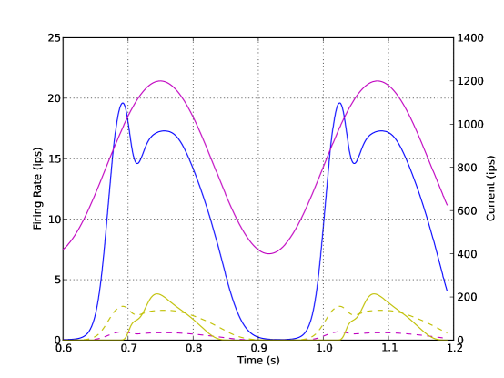
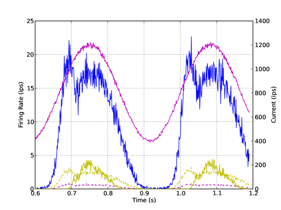
Figure 8: The top and bottom panels show the activities of the excitatory population represented by the population equation, and by the simulation of 9,000 IF neurons. The blue line, scaled on the left axis, plots the firing rate of the population. The magenta and yellow lines represent excitatory and inhibitory currents, respectively; and the solid and dashed lines represent external and feedback currents, respectively. The currents are scaled on the right axis. Note that the similarity between the average firing rate per neuron obtained from the population equation and from the direct simulation (blue lines in the top and bottom panels).

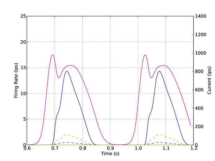
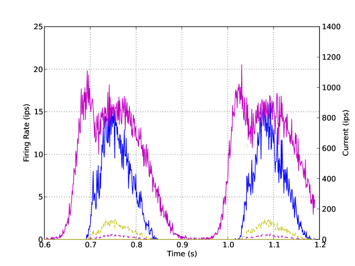
Figure 9: Same as Figure 8 but for the inhibitory population in the two-populations model.

2.3 Partial Conclusions

Given a dynamical model of a neuron, we now know how to derive an EDM for a population of such neurons. For an IF model of a neuron, here we have shown that EDMs accurately approximate population activity (i.e., the pdf of the trans-membrane voltage, $\rho(\upsilon,t)$, and the average firing rate per neuron, $r(t)$). The next step in this sub project is to estimate connectivity parameters (e.g., $W_{ie}$ and $W_{ei}$ in Figure 7) from simulated data.

3 Reducing dimensionality in EDMs

In the previous section we showed that Ensemble Density Models (EDMs) accurately approximated the average firing rate per neuron and the probability density function (pdf) of direct simulations of ensembles of integrate-and-fire (IF) neurons. In networks of EDMs, we want to estimate connectivity parameters and state variables (i.e., the pdfs of the different ensembles) from recorded ensemble firing rates. The state space of each previously reported EDM contained 210 variables. To make the estimation of parameters and state variables in networks of EDMs feasible/efficient it would be helpful to find low-dimensional approximations of EDMs. Here we report the approximation power of one such low-dimensional approximation method. This method was inspired by the moving basis technique in Knight (2000).

3.1 Method to find low-dimensional approximations of EDMs

The evolution of the ensemble pdf, $\rho(\upsilon,t)$, is given by:

$$\dot{\rho}(\upsilon,t)=Q(s(t))\rho(\upsilon,t)$$ (4)

where $Q(s(t))$ is a differential operator that depends on the stimulus $s(t)$. The normalized voltage $\upsilon$ in Equation 4 ranges in the unit interval. To numerically solve this equation, we discretize $\upsilon$, $\{\upsilon_{i}=i/N:1\leq i\leq N\}$ and $\rho$, $\{\rho_{i}(t)=\rho(\upsilon_{i}-\Delta/2,t):1\leq i\leq N\}$, giving a discretization of Equation 4:

$$\dot{\bm{\rho}}(t)=\hat{Q}(s(t))\bm{\rho}(t)$$ (5)

where $\hat{Q}(s(t))\in\mathbb{R}^{N\times N}$ is the matrix representation of the differential operator $Q(s(t)$. Equation 5 is a system of $N$ differential equations. The objective of the dimensionality reduction method described below is to approximate the evolution of $\bm{\rho}(t)$ using a system of $M$ differential equations, where $M\ll N$. For this, the ensemble pdf $\bm{\rho}(t)$ is represented in a basis of eigenvectors of the differential matrix $\hat{Q}(s(t)$, where many coefficients in the new representation can be discarded without much loss in approximation power.

3.1.1 Representing the ensemble pdf in a new basis

Let $\{\phi_{n}(s(t)):0\leq n<N\}$ and $\{\lambda_{n}(s(t)):0\leq n<N\}$ be the eigenvectors and eigenvalues, respectively, of $\hat{Q}(s(t))$:

$$\hat{Q}(s(t))\bm{\phi}_{n}(s(t))=\lambda_{n}(s(t))\bm{\phi}_{n}(s(t))$$ (6)

or in matrix notation:

$$\hat{Q}(s(t))\Phi(s(t))=\Phi(s(t))\Lambda(s(t))$$ (7)

where $\bm{\phi}_{n}(s(t))$ is the nth column of the matrix $\Phi(s(t))$ and $\lambda_{n}(s(t))$ is the nth diagonal element of the diagonal matrix $\Lambda(s(t))$.

Assuming the eigenvectors are linearly independent, we represent $\bm{\rho}(t)$ as:

$$\bm{\rho}(t)=\sum_{n=1}^{N}a_{n}(t)\bm{\phi}_{n}(s(t))$$ (8)

or in matrix notation:

$$\bm{\rho}(t)=\Phi(s(t))\,\mathbf{a}(t)$$ (9)

From Equations 9 and 7 it follows:

$$\hat{Q}(s(t))\bm{\rho}(t)=\hat{Q}(s(t))\Phi(s(t))\,\mathbf{a}(t)=\Phi(s(t))\Lambda(s(t))\,\mathbf{a}(t)$$ (10)

Using a backward difference to approximate the time derivative of $\bm{\rho}(t)$:

$$\dot{\bm{\rho}}(t)=\frac{\bm{\rho}(t)-\bm{\rho}(t-\Delta t)}{\Delta t}$$ (11)

in Equation 5 we obtain:

$$\bm{\rho}(t)-\Delta t\,\hat{Q}(s(t))\bm{\rho}(t)=\bm{\rho}(t-\Delta t)$$ (12)

Now applying Equations 9 and 10 to Equation 12 we get:

$$\left[\Phi(s(t))\left(I-\Delta t\Lambda(s(t))\right)\right]\mathbf{a}(t)=\Phi(s(t-\Delta t)\mathbf{a}(t-\Delta t)$$ (13)

or:

$$\mathbf{a}(t)=\left[\left(I-\Delta t\Lambda(s(t))\right)^{-1}\Phi(s(t))^{-1}\Phi(s(t-\Delta t)\right]\mathbf{a}(t-\Delta t)$$ (14)

Equation 14 provides the evolution of the coefficients $\mathbf{a}(t)$ in Equation 9. It just expresses the evolution of the ensemble pdf in Equation 5 in another basis. It is an exact formula (i.e., it is not an approximation) and has the same dimensionality as Equation 5. The importance of Equation 14 is that one can approximate the evolution of the ensemble pdf by discarding many components of $\mathbf{a}(t)$, as we explain next.

3.1.2 Reducing dimensionality in the new basis

To understand why one can discard many coefficients in the representation of the ensemble pdf of Equation 9 without much loss in approximation power, consider the case where the stimulus, $s(t)$, is constant. In such a case, the eigenvectors and eigenvalues will neither depend on the stimulus; i.e., $\Phi(s(t))=\Phi$ and $\Lambda(s(t))=\Lambda$. Then Equations 5 and 9 reduce to:

$$\dot{\bm{\rho}}(t)=\hat{Q}\bm{\rho}(t)$$ (15)

and:

$$\bm{\rho}(t)=\Phi\,\mathbf{a}(t)$$ (16)

Taking derivatives in Equation 16 we obtain:

$$\dot{\bm{\rho}}(t)=\Phi\,\dot{\mathbf{a}}(t)$$ (17)

and substituing Equation 16 in Equation 15, and applying Equation 7, we get:

$$\dot{\bm{\rho}}(t)=\hat{Q}\Phi\,\mathbf{a}(t)=\Phi\Lambda\,\mathbf{a}(t)$$ (18)

Equating the right hand sides in Equations 17 and 18, and pre multiplying by $\Phi^{-1}$, gives:

$$\dot{\mathbf{a}}(t)=\Lambda\,\mathbf{a}(t)$$ (19)

or:

$$\dot{a_{i}}(t)=\lambda_{i}\,a_{i}(t)$$ (20)

with solution:

$$a_{i}(t)=\exp(\lambda_{i}t)\;a_{i}(0)$$ (21)

Thus, the absolute value of a low dimensional coefficient $a_{i}$ evolves as:

$$|a_{i}(t)|=\exp(\Re(\lambda_{i})t)\;|a_{i}(0)|$$ (22)

Because all eigenvalues have negative real part (with the exception of the zero eigenvalue), the coefficients associated with non-zero eigenvalues will decay to zero, and the speed of this decay will be proportional to the absolute value of the real part of the corresponding eigenvalue. Therefore, to achieve dimensionality reduction in Equation 14 we may discard those coefficients associated with eigenvalues with larger absolute value of their real part, since these coefficients will rapidly decay to zero.

3.2 Evaluation of the method

We first study how well low-dimensional EDMs approximate the average firing rate per neuron in direct stimulations (Section 3.2.1) and then how they approximate the ensemble pdf (Section 3.2.2).

These studies were peformed in data simulated from the network of EDMs illustrated in Figure 7. The network was driven by an excitatory sinusoidal input to the excitatory population (shown by the dotted curve and scaled along the right axis in the top panel of Figure 10). The average firing per neuron in this population, scaled by a constant $W_{ei}=50$, drove the inhibitory population (shown by the dotted curve and scaled along the right axis in the top panel of Figure 11). In turn, the average firing rate per neuron in the inhibitory population, scaled by a constant $W_{ie}=15$, inhibited the excitatory population. Both populations contained feedback (i.e., each neuron received 10 inputs from ten other cells in the same population and 80% of these inputs were inhibitory).

3.2.1 Firing Rates

The top panels of Figures 10 and 11 show the average firing rate per neuron obtained from direct simulation (grey curve), from a full-dimensional EDM (red curve), and from low-dimensional EDMs (the blue, cyan, and red curves correspond to 17, 5, and 1 moving basis, respectively). The full dimensional EDM and its low dimensinal approximations with 17 and 5 moving basis almost perfectly approximate the average firing rate per neuron of the direct simulation. The approximation power of the EDM with only one moving basis is not as good, but it look reasonable.

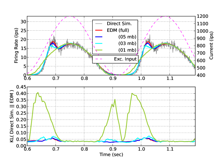
Figure 10: Average firing rate per neuron (top) and KL divergence between the ensemble pdf calculated by direct simulation and that caculated by EDMs (bottom) for the excitatory ensemble.

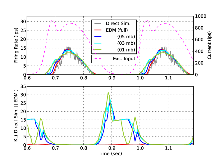
Figure 11: Average firing rate per neuron (top) and KL divergence between the ensemble pdf calculated by direct simulation and that caculated by EDMs (bottom) for the inhibitory ensemble.

3.2.2 Ensemble Proability Density Functions

We compared the normalized histogram of number of directly simulated neuron per voltage bin (i.e., the ensemble pdf from direct simulation) with the pdfs calculated with EDMs (i.e., Equation 5). For this we computed at every time step the Kullback-Leibler (KL) divergence (in bits) between the pdfs obtained by direct stimulation and those obtained from EDMs. These KL divergences are shown in the bottom panels of Figures 10 and 11.

We see that the pdfs obtained from EDMs were good approximation of the pdfs from the direct simulation at times of large average firing rate per neuron (between 0.73 and 0.85 seconds and between 1.03 and 1.2 seconds in the bottom panel of Figure 10, and between 0.72 and 0.82 seconds and between 1.03 and 1.18 seconds in the bottom panel of Figure 11).

At times of low averaged firing rate per neuron the difference between the pdfs obtained from direct simulation and those obtained from EDMs were an order of magnitude larger for the inhibitory than for the excitatory ensemble. This is probably because the excitatory ensemble was driven by a large and smooth sinusoidal input while the inhibitory ensemble was driven by the weaker and non-smooth average firing rate per neuron of the excitatory ensemble. Also, at most time points, the larger the number of moving basis in low-dimensional EDMs, the better the EDM pdf approximated the pdf obtained from direct simulation, as can be seen more clearly in the bottom panel of Figure 11.

To try to understand why the pdfs obtained from direct simulation were different from those obtained from low-dimensional EDMs, we plotted these pdfs for the inhibitory ensemble in an interval of low average firing rate per neuron (from 0.81 seconds in Figure 12 to 1.09 seconds in Figure 26). In the transition between weak to zero average firing rate per neuron (from 0.81 seconds in Figure 12 to 0.93 seconds in Figure 18) the low-dimensional pdfs moved faster towards lowers voltage than the pdfs from the full-dimensional EDM and those from direct simulation. Similarly, in the transition between zero to weak average firing rate per neuron (from 0.95 seconds in Figure 19 to 1.09 seconds in Figure 26) the low-dimensional pdfs moved faster towards higher voltages than the pdfs from the full-dimensional EDM and those from direct simulation. This suggests that the moving basis discarded in the low-dimensional approximations of EDMs help prevent the EDM pdf to transition too fast to and away from the pdf corresponding to large average firing rate per neuron.

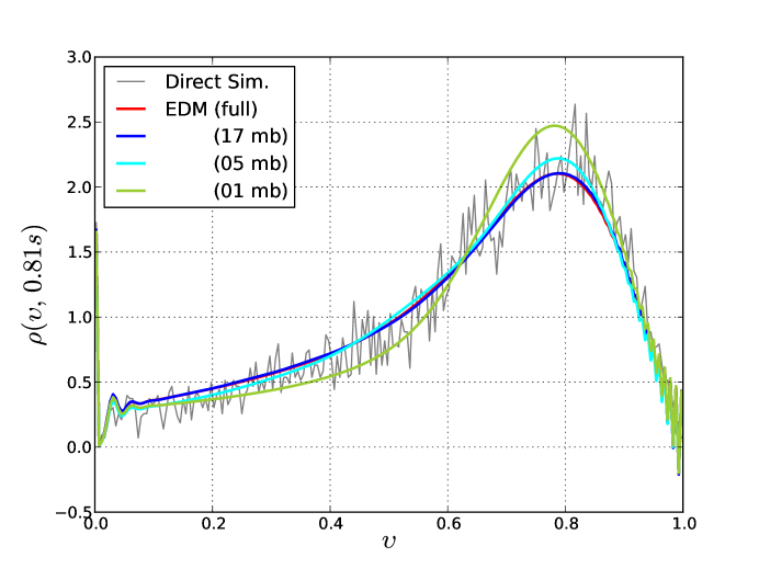
Figure 12: Ensemble pdfs for the inhibitory ensemble at 0.81s.

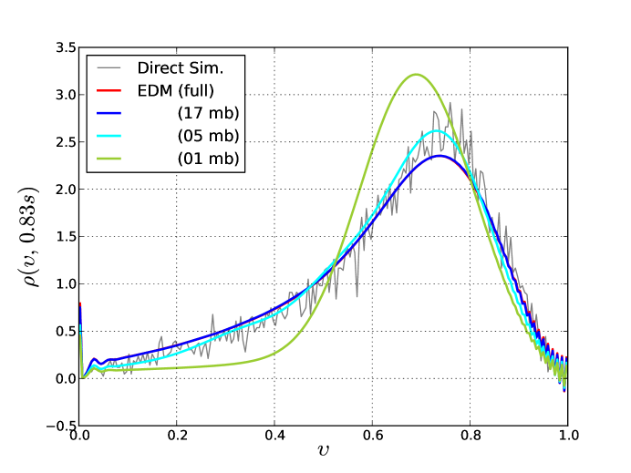
Figure 13: Ensemble pdfs for the inhibitory ensemble at 0.83s.

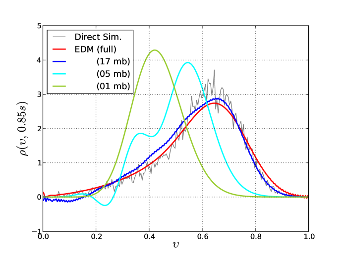
Figure 14: Ensemble pdfs for the inhibitory ensemble 0.85s.

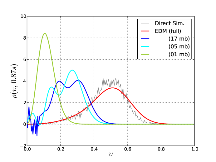
Figure 15: Ensemble pdfs for the inhibitory ensemble 0.87s.

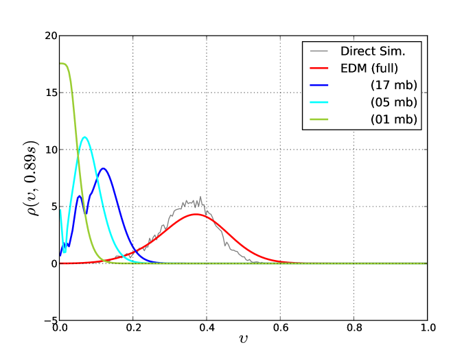
Figure 16: Ensemble pdfs for the inhibitory ensemble 0.89s.

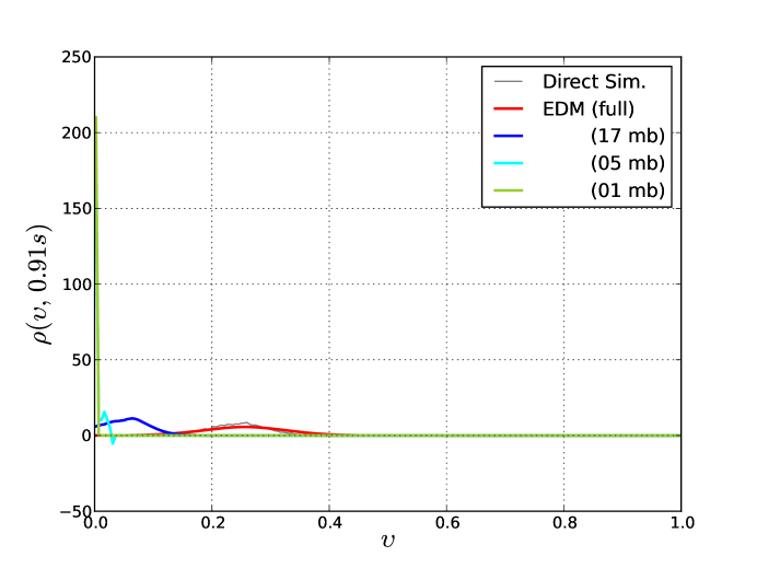
Figure 17: Ensemble pdfs for the inhibitory ensemble 0.91s.

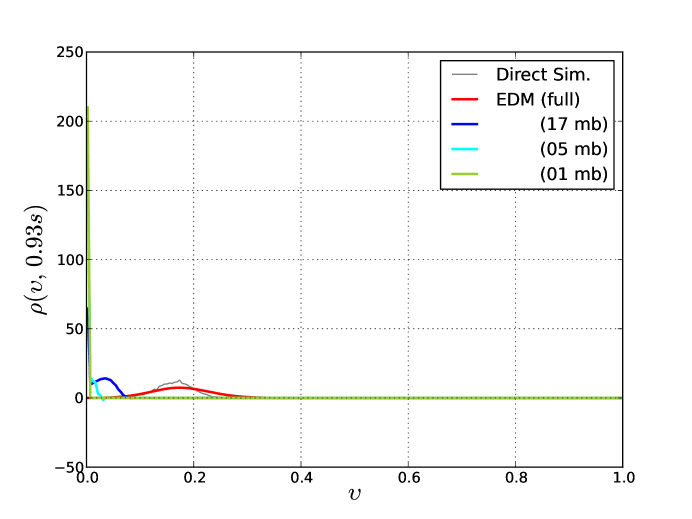
Figure 18: Ensemble pdfs for the inhibitory ensemble 0.93s.

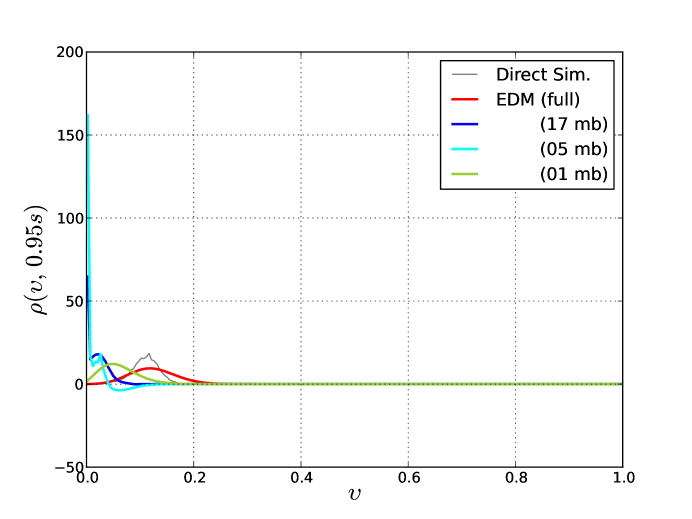
Figure 19: Ensemble pdfs for the inhibitory ensemble 0.95s.

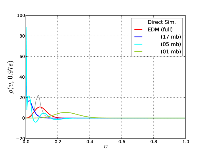
Figure 20: Ensemble pdfs for the inhibitory ensemble 0.97s.

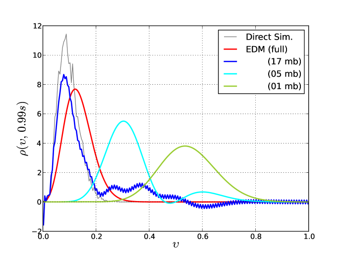
Figure 21: Ensemble pdfs for the inhibitory ensemble 0.99s.

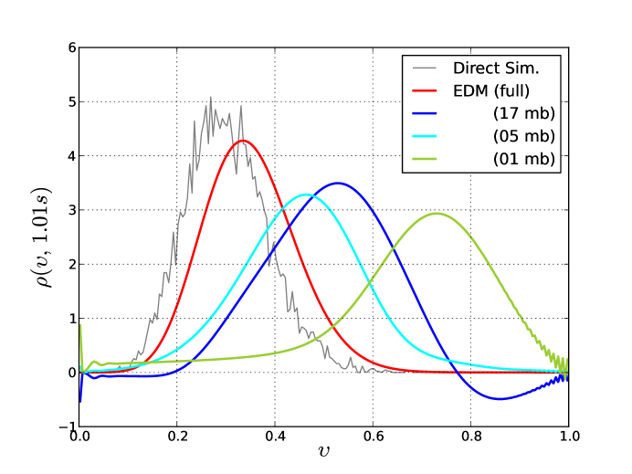
Figure 22: Ensemble pdfs for the inhibitory ensemble 1.01s.

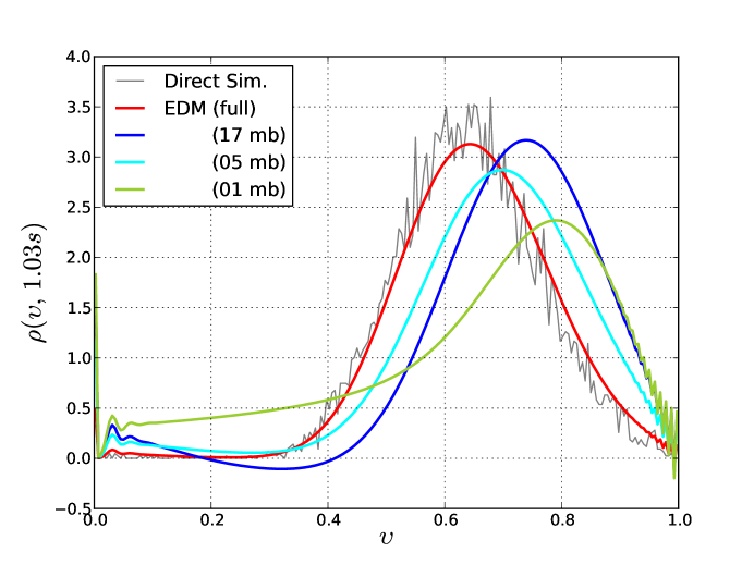
Figure 23: Ensemble pdfs for the inhibitory ensemble 1.03s.

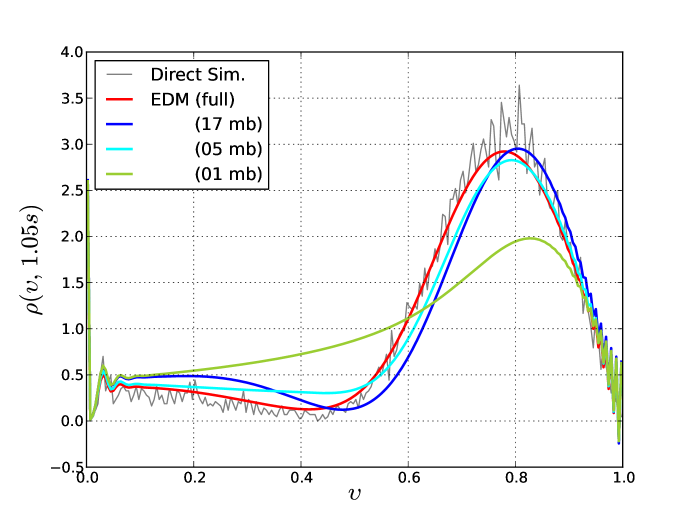
Figure 24: Ensemble pdfs for the inhibitory ensemble 1.05s.

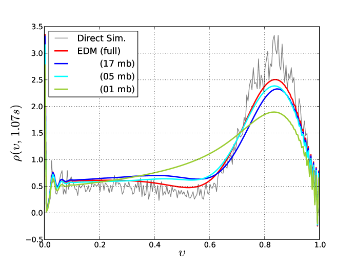
Figure 25: Ensemble pdfs for the inhibitory ensemble 1.07s.

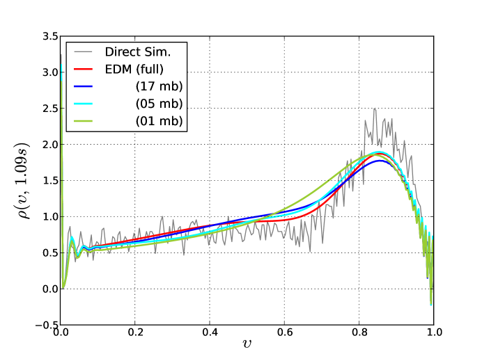
Figure 26: Ensemble pdfs for the inhibitory ensemble 1.09s.

3.3 Partial conclusions

We have developed a method to reduce the dimensionality of the state space of EDMs. We observed that the pdfs from low-dimensional EDMs move faster to and away from the high-average-firing-rate-per-neuron pdf than the pdf derived from direct simulation or that from full EDMS. However, these differences did not have a large impact on the average firing rate per neuron produced by low-dimensional EDMs, which almost perfectly approximates the average firing rate per neuron computed by direct simulation.

Our next step is to estimate connectivity parameters and state space variables in networks of EDMs from recorded spike rates. We will first do this with simulated data.

4 Estimating parameters of EDMs

Here we evaluate a maximum likelihood method to estimate the connectivity parameters $\bm{\theta}=[W_{ei},W_{ie}]$ in the EDMs network in Figure 27. We seek the connectivity parameters for which a set of $N$ pairs measurements, $Y_{N}=[\mathbf{y}(0),\ldots,\mathbf{y}(N-1)]$, are most probable; ie:

Figure 27: Network of EDMs.

$$\bm{\theta}_{ml}=\operatorname*{arg\,max}_{\bm{\theta}}P(Y_{N}|\bm{\theta})$$

The pair of measurements at time $n$, $\mathbf{y}(n)$ comprises measurements from the excitatory and inhibitory ensembles; i.e., $\mathbf{y}(n)=[y_{e}(n),y_{i}(n)]$.

4.1 Noise Model

As a first approximation we make the following three assumptions on the noise of the measurements. These are the assumptions made in previous work by our collaborators (Kostuk et al., 2012).

1. Noise is independent in time; i.e., $P(Y_{N}|\bm{\theta})=\Pi_{n=1}^{N}P(\mathbf{y}(n)|\bm{\theta})$.

2. Noise is independent in the different populations; i.e., $P(\mathbf{y}(n)|\bm{\theta})=P(y_{e}(n)|\bm{\theta})P(y_{i}(n)|\bm{\theta})$.

3. Gaussian noise with a known variance, $\sigma^{2}$, in each population; i.e., $P(y_{.}(n)|\bm{\theta})=N(y_{.}(n)|r_{.}(n|\bm{\theta}),\sigma^{2})$, where $r_{.}(n|\bm{\theta})$ is the activity generated by the ensemble at time $n$.

With these assumptions the log likelihood function of the model parameters reduces to:

$$\log P(Y_{N}|\bm{\theta})=K-\Sigma_{n=0}^{N}\frac{(y_{e}(n)-r_{e}(n|\bm{\theta}))^{2}+(y_{e}(n)-r_{e}(n|\bm{\theta}))^{2}}{2\sigma^{2}}$$

The red lines in Figure 28 plots the activity generated by the excitatory and inhibitory ensemble with connectivity parameters $W_{ei}=50$ and $W_{ie}=15$. The blue lines plot the noisy measurements ($\sigma=2$) that we use below for parameter estimation.

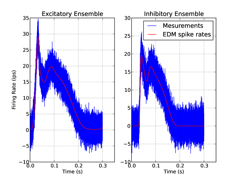
Figure 28: EDMs spike rates (red) and noisy measurements (blue, $\sigma=2$) used to estimate the connectivity parameters in the network of Figure 27.

4.2 Optimization Surface

The levelplot in Figure 29 shows the optimization surface for the set of parameters show in the axes. We see that it has a convex shape with peak at the true parameters. Thus, an iterative gradient-ascent optimization procedure should climb to the maximum-likelihood parameters from any starting set of parameters.

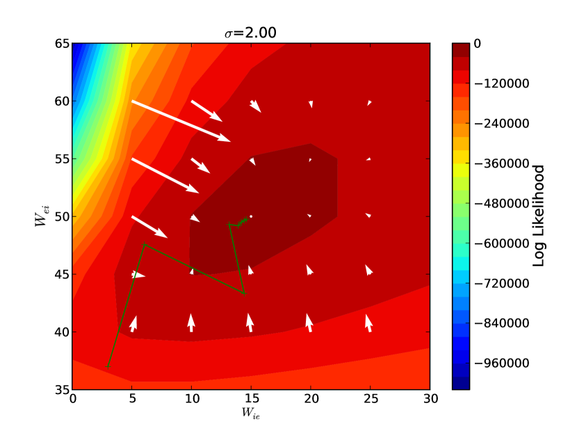
Figure 29: Log-likelihood function, its gradient, and a sample gradient ascent path. The contour plot plots the log-likelihood function for the parameter values shown on the axes for the network in Figure 27. The white arrows show the log-likelihood gradient computed analytically. The green curve is a gradient ascent trajectory starting at $W_{ei}=37$ and $W_{ie}=3$.

4.3 Gradient of Log-Likelihood Function

To compute the gradient of the log-likelihood function at a given set of parameters $\bm{\theta}=[w_{ei}$, $w_{ie}]$ one needs to integrate the EDMs to generate at each time step the activities of both ensembles, $r_{e}(n,\bm{\theta})$ and $r_{i}(n,\bm{\theta})$, as well as the ensembles pdfs, $\bm{\rho}_{e}(n|\bm{\theta})$ and $\bm{\rho}_{i}(n|\bm{\theta})$. With these quantities in hand, the gradient of the log-likelihood function can be computed recursively in a second integration step (Equation 23).

$$\frac{\partial\log P(Y_{m}|\bm{\theta})}{\partial W_{ei}} = \Sigma_{n=0}^{m}\frac{(y_{e}[n]-r_{e}[n;\bm{\theta}])\frac{\partial r_{e}[n;\bm{\theta}]}{\partial W_{ei}}+(y_{i}[n]-r_{i}[n;\bm{\theta}])\frac{\partial r_{i}[n;\bm{\theta}]}{\partial W_{ei}}}{\sigma^{2}}$$

$$\frac{\partial r_{e}[n;\bm{\theta}]}{\partial W_{ei}} = \Delta v\,\sigma_{e}^{E}[n]\,(\mathbf{q}_{r},\frac{\partial\bm{\rho_{e}}[n|\bm{\theta}]}{\partial W_{ei}})$$

$$\frac{\partial\bm{\rho}_{e}[n|\bm{\theta}]}{\partial W_{ei}} = \Delta t\frac{\partial Q_{e}[n-1;\bm{\theta}]}{\partial W_{ei}}\bm{\rho}_{e}[n-1|\bm{\theta}]+\left[I+\Delta t\,Q_{e}[n-1;\bm{\theta}]\right]\frac{\partial\bm{\rho}_{e}[n-1|\bm{\theta}]}{\partial W_{ei}}$$

$$\frac{\partial Q_{e}[n;\bm{\theta}]}{\partial W_{ei}} = -W_{ei}\frac{\partial r_{i}[n-1;\bm{\theta}]}{\partial W_{ei}}A^{(2)}$$ (23)

The white arrows in Figure 29 point in the direction of the gradient, and are scaled according to the gradient magnitude. Note that, as expected, the gradient direction is perpendicular to the level lines.

With a convex log-likelihood function, for which we can compute its gradient, we can now use an iterative gradient ascent procedure to maximize this function. The green line in Figure 29 shows a gradient-ascent trajectory that in only three steps accurately approximated the maximum likelihood parameters.

5 Modeling evoked auditory activity in rodents with EDMs

Here we show that the average firing-rate per neuron predicted by EDMs well approximates the evoked high-gamma power (HGP) from auditory neurons in response to stimulation with pure-tones.

5.1 Recordings

We used very high-resolution simultaneous surface and laminar recordings (Figure 30) in anesthetized rodents stimulated with pure tones at different frequencies and amplitudes. The blue trace in Figure 31 shows the high-gamma power (HGP) evoked by the presentation of tones in one sample electrode of the array. Each vertical dotted color line marks the onset of a tone of a corresponding frequency.

We see that these evoked waveforms are very stereotypical. Some waveforms have a large peak followed by a bump. Other waveforms have two peaks, with a smaller peak preceding a larger one. We also see inf Figure 32 waveforms that have more than one peak preceding a larger one and waveforms having a larger peak followed by a smaller one.

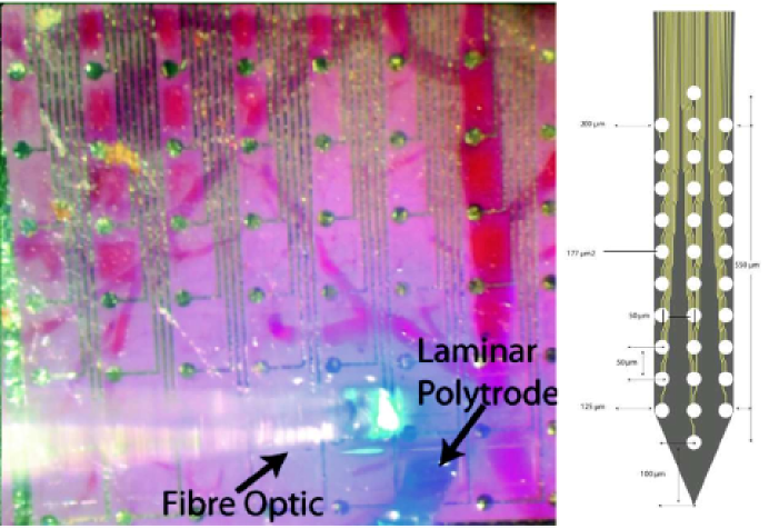
Figure 30: Electrodes used for simultaneous surface and laminar recordings. Surface recordings were obtained from an $8\times 8$ grid of subdurally implanted electrodes covering an area of $1.6~{}mm^{2}$. Laminar recordings were obtained from a 32-channel politrodes of length $650~{}\mu m$. These rercordings were combined with optogenetic manipulations.

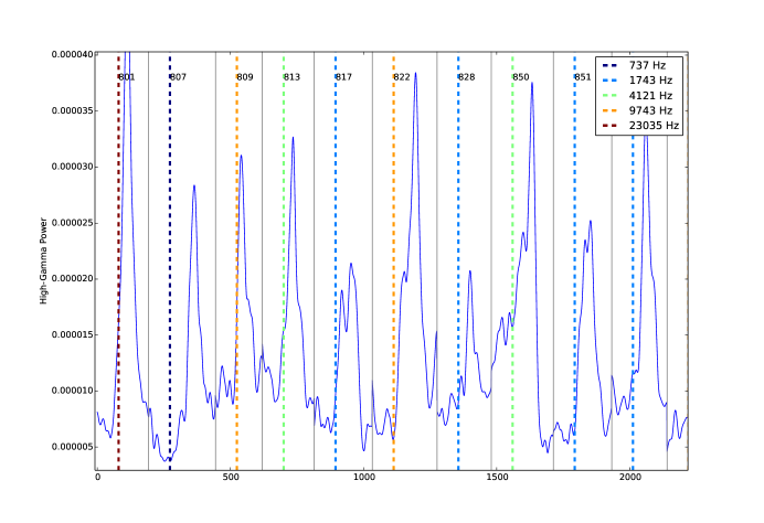
Figure 31: High-gamma power evoked by the presentation of pure tones at different frequencies and amplitudes. Blue traces show the HGP evoked by the presentation of tones in one sample electrode of the array. Each vertical dotted color line marks the onset of a tone of a corresponding frequency.

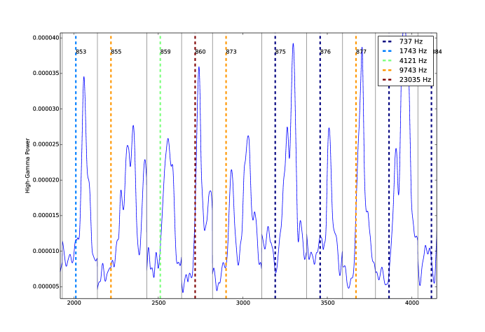
Figure 32: More examples of HGP evoked by the presentation of pure tones. The format is as in Figure 31.

5.2 Qualitative analysis

The recorded HGP waveforms appear remarkably similar to those produced by EDMs when stimulated by sinusoids. To confirm this similarity we manually chose parameters for EDMs to reproduce the shape of recorded waveforms (Figures 33, 34, 35, and 36).

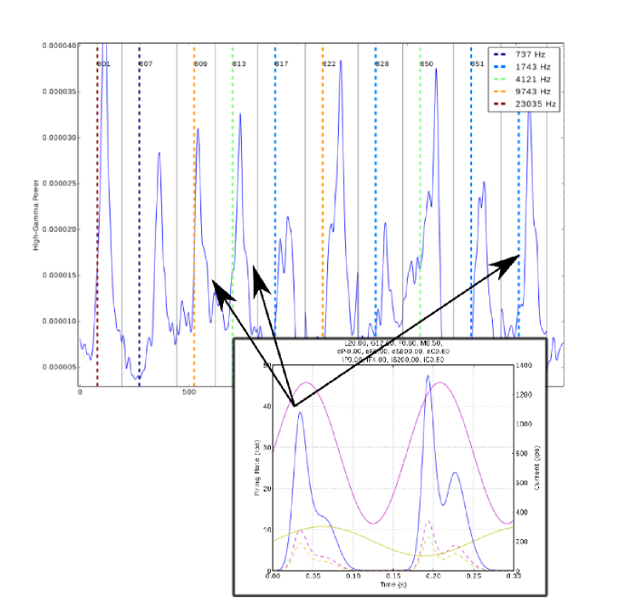
Figure 33: The blue curve in the inset shows the average firing-rate simulated by an EDM with manually chosen parameters. The magenta and yellow solid curves plot its excitatory and inhibitory inputs, respectively. The first waveform is qualitatively similar to the ECoG waveforms with a bump following a large peak.

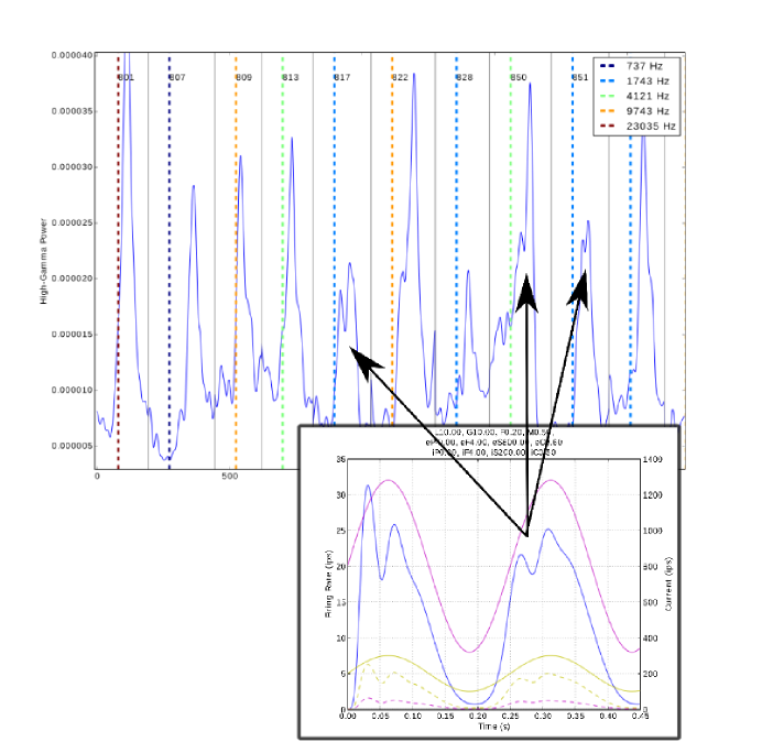
Figure 34: The blue curve in the inset shows the average firing-rate simulated by an EDM with manually chosen parameters. The magenta and yellow solid curves plot its excitatory and inhibitory inputs, respectively. The second waveform is qualitatively similar to the ECoG waveforms with a lower peak preceding a large one.

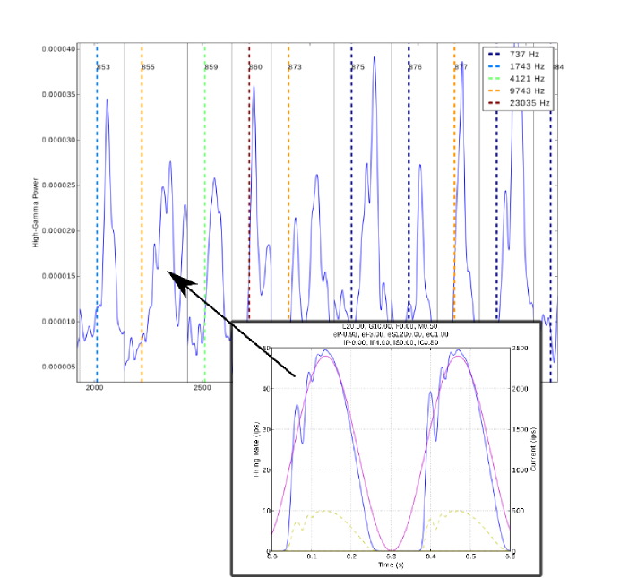
Figure 35: The blue curve in the inset shows the average firing-rate simulated by an EDM with manually chosen parameters. The magenta and yellow solid curves plot its excitatory and inhibitory inputs, respectively. EDMs can generate waveforms with multiple lower peaks preceding a larger one.

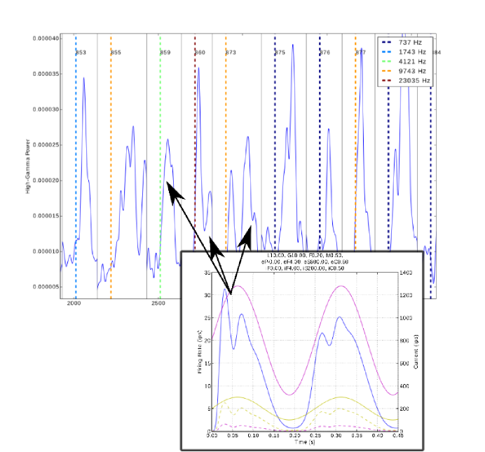
Figure 36: The blue curve in the inset shows the average firing-rate simulated by an EDM with manually chosen parameters. The magenta and yellow solid curves plot its excitatory and inhibitory inputs, respectively. EDMs can generate waveforms with a larger peak preceding a smaller one.

5.3 Quantitative analysis

Using a similar method as described above to learn connectivity parameters in networks of EDMs, we etimated parameters so that an EDM approximated as close as possible the HGP evoked by the presentation of pure tones to rodents. In total we estimated 13 parameters: three parameters of an EDM, two parameters for its initial condition, four parameters for the sinusoidal excitatory input, and four parameters for the inhibitory input. The recorded and approximated HGP are given by the blue and red solid curves, respectively, in Figure 37.

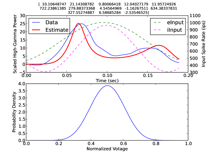
Figure 37: Learning ensemble properties to approximate physiological recordings. We estimated 13 parameters so that the average firing rate per neuron predicted by an EDM approximates as close as possible the recorded HGP in response of a pure tone. The title shows the values of these parameters. The blue and red curves in the top panel plot the recorded HGP and the predicted average firing rate per neuron, respectively. The dotted green and magenta curves in the top panel shows the estimated excitatory and inhibitory inputs to the EDM. The curve in the bottom panel plot the estimated initial condition probability density function of the EDM. The average firing rate predicted by the EDM is a good approximation of the recorded HGP.

5.4 Partial Conclusions

These preliminary results show that EDMs, besides accurately approximating the average firing rate of ensembles of simulated IF neurons, well approximate the HGP in the auditory cortex of rats evoked by auditory tones.

6 Conclusions

We have shown that an ensemble model accurately reproduce the probability density function of the transmembrane voltage, as well as the average-firing rate per neurona, in a large ensemble of integrate-and-fire simulated neurons (Section 2). We developed and evaluated methods to reduce the dimensionality (Section 3) and estimate parameters (Section 4). Finally we demonstrated the feasibility of EDMs to model the high-gamma power evoked by pure tones in the auditory cortex of rodents.

The possiblity of quantitatively model the activity of ensemble of neurons may allow us to uncover fundamental computations performed by neural ensembles.

References

- Knight [2000] B.W. Knight. Dynamics of encoding in neuron populations: some general mathematical features. Neural Computation, 12:473–518, 2000.
- Kostuk et al. [2012] M. Kostuk, B.A. Toth, C.D. Meliza, D. Margoliash, and H.D.I. Abarbanel. Dynamical estimation of neuron and network properties II: path integral monte carlo methods. Biological Cybernetics, 106:155–167, 2012.
- Omurtag et al. [2000] A. Omurtag, B.W. Knight, and L. Sirovich. On the simulation of large populations of neurons. Journal of Computational Neuroscience, 8:51–63, 2000.