Rayleigh-Taylor Unstable Flames – Fast or Faster?

Abstract

Rayleigh-Taylor (RT) unstable flames play a key role in the explosions of Type Ia supernovae. However, the dynamics of these flames is still not well-understood. RT unstable flames are affected by both the RT instability of the flame front and by RT-generated turbulence. The coexistence of these factors complicates the choice of flame speed subgrid models for full-star Type Ia simulations. Both processes can stretch and wrinkle the flame surface, increasing its area and, therefore, the burning rate. In past research, subgrid models have been based on either the RT instability or turbulence setting the flame speed. We evaluate both models, checking their assumptions and their ability to correctly predict the turbulent flame speed. Specifically, we analyze a large parameter study of 3D direct numerical simulations of RT unstable model flames. This study varies both the simulation domain width and the gravity in order to probe a wide range of flame behaviors. We show that RT unstable flames are different from traditional turbulent flames: they are thinner, rather than thicker when turbulence is stronger. We also show that none of several different types of turbulent flame speed models accurately predicts measured flame speeds. In addition, we find that the RT flame speed model only correctly predicts the measured flame speed in a certain parameter regime. Finally, we propose that the formation of cusps may be the factor causing the flame to propagate more quickly than predicted by the RT model.

I. Introduction

Type Ia supernovae are extremely bright stellar explosions that are not only fascinating in their own right, but also play an important role in cosmological distance measurements (Riess et al., 1998; Perlmutter et al., 1999). Type Ia supernovae are thought to be white dwarf stars that explosively burn their carbon and oxygen into heavier elements, including ${}^{56}\text{Ni}$. The radioactive decay of the ${}^{56}\text{Ni}$, in turn, produces the light seen as the Type Ia explosion. Recent observations of SN 2011fe support the white dwarf explosion scenario (Nugent et al., 2011; Bloom et al., 2012; Brown et al., 2012) but there is still debate about whether the Type Ia supernova progenitor is two merging white dwarfs (the double-degenerate scenario), for example, see Iben & Tutukov (1984); Webbink (1984); Hicken et al. (2007); Yoon et al. (2007); Raskin et al. (2012); Piro et al. (2014), or a single white dwarf driven to explosion by material accreted from a companion star (the single-degenerate scenario), for example, see Whelan & Iben (1973); Nomoto (1982); Iben & Tutukov (1984); Marietta et al. (2000). In this paper, we will focus on how the Rayleigh-Taylor instability affects thermonuclear burning in the single-degenerate scenario.

In the single-degenerate scenario, a white dwarf accretes material from a companion star until its mass approaches the Chandrasekhar limit. During this process, the white dwarf becomes more compact until, somehow, a thermonuclear runaway is triggered. Burning engulfs the star and it explodes. In one scenario, thermonuclear burning is initially triggered in a convective region near the center of the star and then propagates outward (Woosley et al., 2007; Nonaka et al., 2012). The thermonuclear burning is expected to take the form of a very thin front that initially propagates at subsonic speeds. This is known as a deflagration. It was once thought that the deflagration might be enough to trigger the observed supernova explosion, but it has since been shown that a deflagration-only event does not produce an energetic-enough explosion and results in incorrect spectra, with low-velocity carbon and oxygen components (Gamezo et al., 2003, 2004). If, however, the deflagration is sped up until it becomes a self-sustaining, supersonic burning wave (a detonation), then a more realistic explosion is predicted. This more realistic scenario is known as the deflagration-to-detonation transition (DDT) and forms the basis of many different single-degenerate Type Ia explosion scenarios including the standard DDT (Blinnikov & Khokhlov, 1986; Woosley, 1990; Khokhlov, 1991; Khokhlov et al., 1997a, b; Gamezo et al., 2004; Röpke & Niemeyer, 2007), pulsational detonations (Khokhlov, 1991; Arnett & Livne, 1994a, b; Hoeflich et al., 1995; Hoeflich & Khokhlov, 1996; Bravo & García-Senz, 2006), and gravitationally confined detonations (Plewa et al., 2004; Jordan et al., 2008; Meakin et al., 2009; Seitenzahl et al., 2009; Jordan et al., 2012). The cause of the detonation remains an open question; traditionally, the Zel’dovich gradient mechanism has been invoked (Khokhlov et al., 1997a, b), but Poludnenko et al. (2011) have recently identified other processes that can trigger unconfined detonations. Finally, it has been shown that a detonation-only explosion produces too much nickel and iron and can be ruled out (Arnett, 1969; Khokhlov et al., 1993; Filippenko, 1997; Gamezo et al., 1999). Although it could occur in many ways, a DDT is necessary for a realistic Type Ia explosion.

In single-degenerate explosion scenarios, the initial deflagration is Rayleigh-Taylor (RT) unstable (Rayleigh, 1883; Taylor, 1950) because dense fuel sits above lighter burnt ashes in the star’s gravitational field. The RT instability affects the flame in two different ways: first, it stretches the flame surface; second, the nonlinear evolution of this stretching process generates turbulence behind the flame front, which back-reacts on the flame surface, wrinkling it further (Vladimirova & Rosner, 2005; Zhang et al., 2007; Hicks & Rosner, 2013). Both stretching and wrinkling increase the surface area of the flame, speeding it up. As the flame speeds up, it may eventually undergo a DDT. The details of the DDT, in particular, when and how the transition to detonation occurs, determine critical observables such as nickel production (Gamezo et al., 2003, 2004, 2005; Röpke & Niemeyer, 2007; Krueger et al., 2012; Seitenzahl et al., 2013). This transition is still not understood, but one possibility, the Zel’dovich gradient mechanism (Zel’dovich et al., 1970), depends critically on the details of the conditions produced by the deflagration (Khokhlov et al., 1997a, 1999; Oran & Gamezo, 2007; Röpke, 2007; Röpke & Niemeyer, 2007). Without a full understanding of RT unstable flames, the mechanism and final nickel yields of this class of Type Ia supernovae models will remain uncertain.

Ideally, the propagation of RT-unstable flames and the DDT would be studied using full-star simulations. However, the separation of scales in the problem makes this unfeasible: the size of the star (approximately Earth-sized) is much too large relative to the width of the flame ($10^{-4}$ to $10^{2}$ cm according to Timmes & Woosley (1992)) to resolve both in the same simulation (Oran, 2005). Instead, full-star simulations must include a variety of subgrid models, including, in particular, a subgrid model that gives the speed of the flame below certain scales. There are two basic types of subgrid model, and there has been a long debate about which of the two is correct. Each model incorporates a different assumption about how RT-unstable flames should behave. In one, the turbulent flame speed is set by the Rayleigh-Taylor instability. In the other, the interactions of turbulence with the flame front dictate the flame speed. The question at the heart of this and prior research (Hicks & Rosner, 2013) is whether both or either of these two deflagration subgrid models is physically appropriate.

RT-type subgrid scale (RT-SGS) models (Khokhlov, 1995; Khokhlov et al., 1996; Gamezo et al., 2003, 2004, 2005; Zhang et al., 2007; Townsley et al., 2007; Jordan et al., 2008) are based on the hypothesis that the RT stretching of the flame front sets the turbulent flame speed. In these models, the turbulent speed of the flame on an unresolved scale $\Delta$ is given by the velocity $v_{RT}(\Delta)\propto\sqrt{g\,A\,\Delta}$ which is naturally associated with the Rayleigh-Taylor instability at the length scale $\ell=\Delta$. Here $g$ is the gravitational acceleration and the Atwood number is $A=(\rho_{\rm fuel}-\rho_{\rm ash})/(\rho_{\rm fuel}+\rho_{\rm ash})$, where $\rho_{\rm fuel}$ and $\rho_{\rm ash}$ are the densities of the fuel and the ash. Two major hypotheses underlie the RT-type subgrid model: self-similarity and self-regulation. Self-similarity means that the flame is effectively a fractal, so the RT subgrid model applies at any scale. Self-regulation means that physical processes will force the flame back towards the RT flame speed if the flame starts to move too fast or too slow. Self-regulation is a competition between two processes, the creation of flame surface area by the RT instability (which increases the turbulent flame speed) and destruction of flame surface area by cusp burning (which decreases the turbulent flame speed); cusps are areas of the flame surface with high curvature. As the flame develops small wrinkles, due to turbulence or the RT instability, cusp burning ensures that these wrinkles will be destroyed, returning the flame speed to the RT predicted value. Likewise, if wrinkle destruction is too effective, the flame front becomes flatter and the RT instability more efficiently increases the surface area and the flame speed. The net result is that the flame is forced to travel at the RT value.

On the other hand, turbulence-based subgrid scale (Turb-SGS) models are based on the hypothesis that flame behavior is determined by the interaction between turbulence and the flame front (Niemeyer & Hillebrandt, 1995; Niemeyer & Woosley, 1997; Niemeyer & Kerstein, 1997; Reinecke et al., 1999; Röpke & Hillebrandt, 2005; Schmidt et al., 2006a, b; Jackson et al., 2014). These models do not distinguish between different sources of turbulence or whether the turbulence is upstream or downstream of the flame front. Turb-SGS models are adapted from the field of turbulent premixed combustion, which studies the propagation of premixed flames (in various configurations) through pre-existing turbulence. In these models, the turbulent flame speed is often based on the root-mean-square (rms) velocity of the pre-existing, upstream turbulence. The key assumption behind astrophysical Turb-SGS models is that flames interact with upstream and downstream turbulence in the same way. One purpose of this paper is to test that assumption.

An exploding white dwarf has two potential sources of turbulence: turbulence produced by the convection that precedes ignition and turbulence produced by the RT-unstable flame front. If the pre-ignition core convection is strongly turbulent, then the flame will travel through this pre-existing turbulence. In that case, the flame is forced to interact with every turbulent eddy it encounters as it propagates upstream. This is exactly the case studied by traditional turbulent premixed combustion, so models from that field are good candidates for Turb-SGS models for Type Ia simulations. The second source of turbulence is the RT instability of the flame front. As the RT instability deforms the flame front, the flame front produces turbulence baroclinically. Previous studies have shown that this turbulence exists only downstream of the flame front (Vladimirova & Rosner, 2003, 2005; Schmidt et al., 2006b; Hicks & Rosner, 2013). The flame will not necessarily interact with this turbulence because it does not need to travel through the turbulent region in order to propagate upstream. In this case, Turb-SGS models based on ideas from traditional turbulent combustion may not apply because the physical situation is fundamentally different. We will not address the question of whether substantial pre-existing turbulence exists in the white dwarf, see Zingale et al. (2009); Nonaka et al. (2012).

The only way to determine which, or even whether, either type of subgrid model is correct is to directly study RT-unstable flames. There have been many such studies, which can be organized by various criteria including dimensionality, resolution requirements, flame type, evolution time and flame regime. 2D simulations (Bell et al., 2004; Vladimirova & Rosner, 2003, 2005; Zhang et al., 2007; Biferale et al., 2011; Hicks & Rosner, 2013) are less computationally expensive than 3D simulations and can cover a wider range of parameter space, but do not produce realistic turbulence. 3D simulations (Khokhlov, 1994, 1995; Zingale et al., 2005b; Zhang et al., 2007; Ciaraldi-Schoolmann et al., 2009; Chertkov et al., 2009) treat the turbulence correctly, but are more computationally expensive. Simulations also differ in what scale is resolved: some use a subgrid model themselves (Ciaraldi-Schoolmann et al., 2009), others resolve the Gibson scale and the flame width (Bell et al., 2004; Zingale et al., 2005b), and still others resolve down to the viscous scale (Vladimirova & Rosner, 2003, 2005; Chertkov et al., 2009; Hicks & Rosner, 2013). RT-unstable flame studies also use different treatments for the flame itself, from realistic carbon-oxygen flames (Bell et al., 2004; Zingale et al., 2005b; Ciaraldi-Schoolmann et al., 2009) to thickened flames in a degenerate setting (Zhang et al., 2007) to model flames in a Boussinesq setting (Vladimirova & Rosner, 2003, 2005; Chertkov et al., 2009; Hicks & Rosner, 2013). Carbon-oxygen flames are most realistic and directly applicable to supernovae, but model flames can better isolate specific effects, such as RT stretching. Another difference between studies is whether they focus on the early, transient stages of RT-unstable flame growth (Bell et al., 2004; Zingale et al., 2005b; Zhang et al., 2007; Chertkov et al., 2009) or later, saturated stages when the flame speed varies around a statistically steady average (Vladimirova & Rosner, 2003, 2005; Zhang et al., 2007; Hicks & Rosner, 2013). In simulations, the saturated stage is reached when the RT instability can no longer grow horizontally due to confinement by the sides of the simulation domain. In this case, a balance develops between RT growth, which creates surface area, and burning, which destroys it. It is likely that RT flame propagation in the star is not statistically steady because there is no confinement mechanism for RT modes and the star expands as the flame propagates; however, it is still not known whether unconfined flames can saturate. So, which choice is more physically relevant – statistically unsteady or saturated simulations – remains unclear. Even if the flame behavior is only transient in the star, saturated simulations indicate the statistically steady state the flame is approaching, even if it never reaches it. The effect of boundary conditions on simulated RT unstable flames have been specifically studied by Vladimirova & Rosner (2003, 2005); Hicks (2014). Finally, simulations vary in what parameter values they use and which combustion regime they probe: flamelets (Bell et al., 2004; Zingale et al., 2005b; Vladimirova & Rosner, 2003, 2005; Zhang et al., 2007; Hicks & Rosner, 2013), thin reaction zones (Bell et al., 2004; Zingale et al., 2005b; Chertkov et al., 2009) or broken reaction zones (Chertkov et al., 2009).

Other facets of burning in white dwarfs have been addressed in other types of studies. If the turbulence generated by the initial convective stage in the white dwarf is strong, then the flame may be dominated by its propagation through this pre-existing turbulence instead of by the RT instability or by the turbulence produced by the RT instability. In that case, traditional ideas and studies of turbulent combustion would be clearly applicable to the formulation of subgrid models. A small selection of the applicable papers, some with specific reference to the Type Ia problem, include: Aspden et al. (2008, 2010); Poludnenko & Oran (2010); Poludnenko et al. (2011); Poludnenko & Oran (2011); Hamlington et al. (2011); Aspden, Day, & Bell (2011); Hamlington et al. (2012); Chatakonda et al. (2013). Even if the flame does not move into a strongly convective field, the turbulence from the carbon flame could influence the trailing oxygen flame; this scenario has been studied by Woosley, Kerstein, & Aspden (2011) and Aspden, Bell, & Woosley (2011). Finally, it is likely that, after ignition takes place near the core of the white dwarf, subsequent burning may take the form of rising buoyant plumes or bubbles (the surfaces of which would be RT unstable). The dynamics of these plumes has been studied by Vladimirova (2007); Zingale & Dursi (2007) and Aspden, Bell, Dong, & Woosley (2011).

In this paper, we will test the basic predictions of RT-SGS and Turb-SGS models against a large parameter study of 3D, fully-resolved, RT unstable model flames. To date, there have been few 3D simulations of RT unstable flames (Khokhlov, 1994, 1995; Zingale et al., 2005a; Zhang et al., 2007; Chertkov et al., 2009), and no parameter studies large enough to clearly test the scaling laws predicted by the subgrid models. In particular, this is the first set of 3D model flame simulations in the flamelet regime that fully resolve the viscous scale. Resolving the viscous scale accounts for all possible interactions between the flame and turbulence in the simulations (for a similar 2D study see Hicks & Rosner (2013)). The set of eleven simulations discussed in this paper tests the scaling laws over a wide range of flame behavior, from a steady rising bubble to a flame highly disturbed by the RT instability. In particular, we will focus on flames in the flamelet regime, a regime in which Type Ia flames are expected to spend a considerable fraction of their time. In addition, we will look for a transition from the flamelets regime to the reaction zones regime, as predicted by traditional turbulent combustion theory. This transition is important because it could lead to conditions that may cause a detonation.

In order to isolate the effects of the RT instability on the flame front, we made as many simplifications to our parameter study setup as possible. In doing this, we neglected many of the complexities of real white dwarf flames. For example, we used a simple model reaction instead of a full chemical reaction chain. We used the Boussinesq approximation and therefore ignored compressibility effects and sound waves. These simplifications allow us to focus directly on the effect that gravity has on the flame without having to disentangle it from other effects like the Landau-Darrieus instability. Finally, we focused on the saturated state, in which quantities such as the flame speed vary around a statistically steady average in order to obtain robust scalings that don’t depend on time.

In this paper, we will test the predictions of the two types of subgrid models both indirectly and directly. To start, in Section II, we describe the problem formulation, the control parameters that are varied in the parameter study and provide a list of the simulations. Next, in Section III, we discuss the different combustion regimes predicted by traditional turbulent combustion theory, and compare the predictions of this theory with observations from our simulations. In particular, we show that the flame remains in the flamelets regime after it is predicted to transition to the reaction zones regime and that the flame becomes thinner instead of thicker when turbulence is strong. Then, in Section IV, we test the predictions of both types of subgrid models, beginning with three types of turbulence-based subgrid models and ending with the predictions of the Rayleigh-Taylor subgrid model. After showing that all of these models fail in certain regions of parameter space, we will (in Subsection IV.6) consider the possibility that the formation of cusps by turbulence and/or the Rayleigh-Taylor instability might explain these deviations. Finally, we draw some conclusions in Section V.

II. Problem Formulation

To isolate the effects of the Rayleigh-Taylor instability on the flame front, we simulated a simple model flame. This model makes two major simplifications to more realistic treatments of nuclear burning: one simplification to the fluid equations themselves, and one simplification to the treatment of the reaction. To simplify the fluid equations, we employ the Boussinesq approximation, which reduces the fully compressible Navier-Stokes equations to an incompressible form. To simplify the reaction, we use a simple model reaction which avoids the intricacies of a full reaction chain.

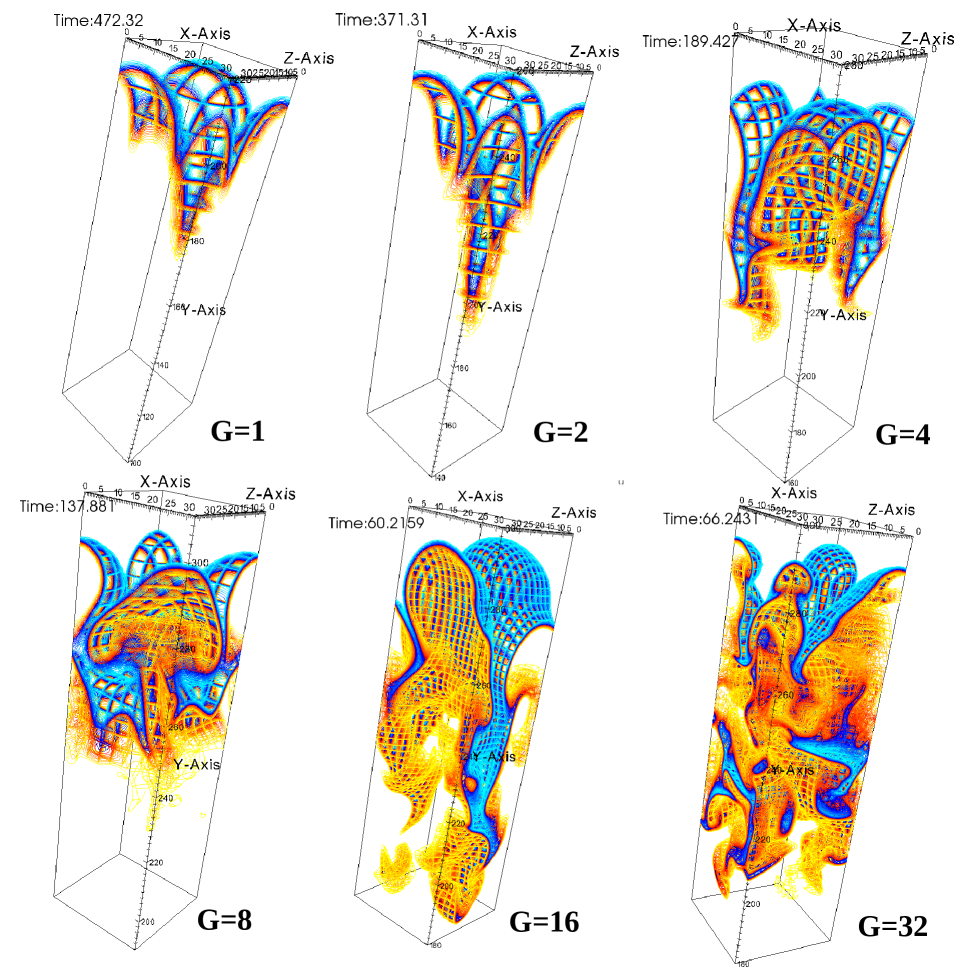
Figure 1.— Contour Plots of Temperature, L=32. This figure shows a sample contour plot of temperature for each of the six simulations with domain size $L=32$. Blue colors represent mostly unburnt fuel and red/yellow colors represent mostly burned ashes. A colorbar showing the assignment of colors to temperatures is shown in Figure 2. Each flame is propagating in the $y$-direction, against the force of gravity which points in the $-y$ direction. In general, the flame surface shape changes with time, causing the flame speed to vary. Note that the flame shape ranges from a simple rising bubble at $G=1$ to a complex, highly convoluted surface at $G=32$. Simulation A, discussed in Section IV.6, is the $G=16$ plot in this figure.

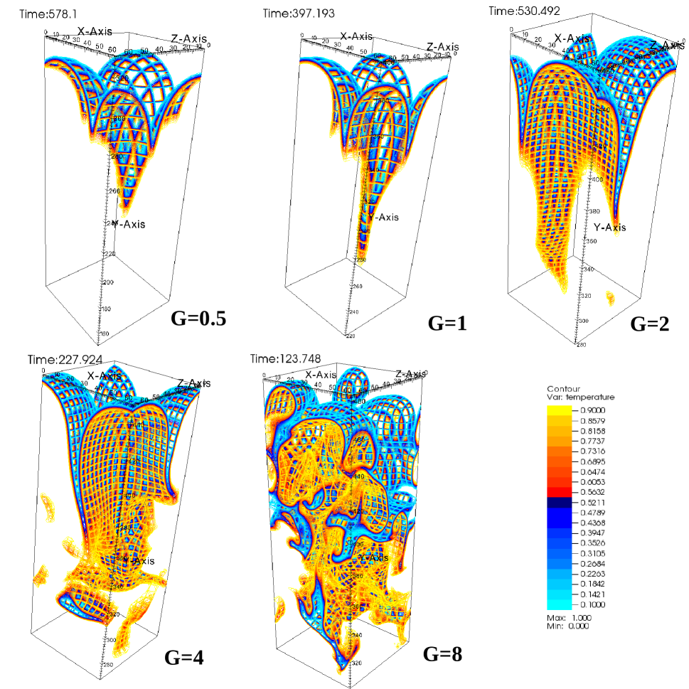
Figure 2.— Contour Plots of Temperature, L=64. This figure shows a sample contour plot of temperature for each of the five simulations with domain size $L=64$. Note that, similarly to Figure 1, the flame shape ranges from a simple rising bubble at $G=0.5$ to a complex, highly convoluted surface at $G=8$. Simulation B, discussed in Section IV.6, is the $G=8$ plot in this figure.

The Boussinesq approximation is appropriate for subsonic flows with only small density (and temperature) variations and a small vertical extent compared to the scale height of the system (Spiegel & Veronis, 1960). If these criteria are fulfilled then a simplified set of equations can be derived, in which the density differences in the flow are taken into account only in the gravity-dependent buoyancy forcing term in the Navier-Stokes equation. For combustion, the density across the flame front $\Delta\rho$ is only included in the forcing term; all other terms depend only on the density of the unburnt fuel, $\rho_{o}$. In this approximation, the continuity equation is incompressible. The Boussinesq approximation disallows shocks and heating due to the viscous dissipation of energy. A flame front may be Rayleigh-Taylor unstable (because gravitational forcing due to density variations in the flow is accounted for in the buoyancy term) but can not be Landau-Darrieus unstable (because density variations are not accounted for outside of the buoyancy term). All of these simplifications are desirable so that the RT instability can be considered without other complications.

The second simplification is that we added a simple reaction term, $R(T)$, to the advection-diffusion-reaction (ADR) temperature equation to replace all of the details of realistic nuclear burning. In this model, $T$ is a reaction progress variable that tracks the state of the fluid from unburnt fuel at $T=0$ to burnt ashes at $T=1$. The reaction progress variable represents both the mass fraction of the burned material and the fraction of energy released into the flow (Vladimirova et al., 2006). In using this model, we do not consider any specific chain of nuclear reactions or the separate evolution of nuclear species and temperature. Instead, the ADR equation models both temperature and species evolution. This simplified approach has been used by many other combustion studies and possible choices for $R(T)$ include the Kolmogorov-Petrovkii-Piskunov (KPP), mth-order Fisher, bistable, Arrhenius and ignition reactions (a review of model reaction types is given by Xin (2000)). In this study we chose $R(T)=2\alpha T^{2}(1-T)$, a bistable reaction with an ignition temperature of zero which, therefore, has no bistable behavior. We choose this particular reaction instead of the more physically realistic Arrhenius reaction because the reaction front is wider and therefore easier to resolve (see also Hicks & Rosner (2013)). We did not choose the KPP reaction used by Vladimirova & Rosner (2003, 2005) because the KPP flame front is very wide and the KPP reaction has an unstable fixed point at $T=0$ which makes it more numerically unstable.

Table 1Simulation Parameters

$G$	$L$	Physical Size	Elements	Order	DOF	Resolution	Time	Time Step ($10^{-3}$)
1	32	32 x 512 x 32	4 x 64 x 4	8	524288	1.000	504.06	30
2	32	32 x 576 x 32	4 x 72 x 4	10	1152000	0.800	429.63	64.801
4	32	32 x 576 x 32	8 x 144 x 8	7	3161088	0.571	250.22	18.051
8	32	32 x 608 x 32	8 x 152 x 8	11	12947968	0.364	157.71	6.659
16	32	32 x 608 x 32	16 x 304 x 16	7	26693632	0.286	75.561	3.665
32	32	32 x 640 x 32	16 x 320 x 16	9	59719680	0.222	87.16	1.99
0.5	64	64 x 640 x 64	8 x 80 x 8	8	2621440	1.000	705.03	15
1	64	64 x 704 x 64	8 x 88 x 8	8	2883584	1.000	440.92	65.071
2	64	64 x 768 x 64	16 x 192 x 16	7	16859136	0.571	606.63	13.031
4	64	64 x 832 x 64	16 x 208 x 16	9	38817792	0.444	300.39	6.924
8	64	64 x 832 x 64	16 x 208 x 16	11	70873088	0.364	173.48	4.316

Note. — Simulation Parameters. The columns are: the nondimensional gravity, the nondimensional domain size, the physical size, the number of elements ($N_{x}$ x $N_{y}$ x $N_{z}$), the polynomial order ($p_{o}$), the number of degrees of freedom ($\sim N_{x}N_{y}N_{z}p_{o}^{3}$), the average resolution (the average spacing between collocation points), the total running time, the time step. All quantities are in nondimensional units.

The bistable reaction has a simple, laminar solution in a stationary, gravity-free fluid (Constantin et al., 2003). When the flame is laminar, it is planar with a characteristic width of $\delta$ and it travels with the laminar flame speed $s_{o}$. $\delta$ and $s_{o}$ are set by $\alpha$, the laminar reaction rate, and $\kappa$, the thermal diffusivity, such that $s_{o}=\sqrt{\alpha\kappa}$ and $\delta=\sqrt{\dfrac{\kappa}{\alpha}}$. The actual flame thickness ($\delta_{t}$), also called the thermal flame width, is larger than the characteristic flame width ($\delta$) by a factor of 4 ($\delta_{t}=4\delta$) as calculated by measuring the distance between the level sets $T=0.1$ and $T=0.9$. Finally, $\delta_{i}$ is the width of the flame reaction zone, the part of the flame in which the most intense burning takes place. This is typically 2-10 times smaller than the laminar flame width.

The fluid equations were non-dimensionalized by the characteristic length scale (the laminar flame front thickness, $\delta$) and time scale in the problem (the reaction time, $1/\alpha$) (Vladimirova & Rosner, 2003) to give

$$\dfrac{D\textbf{u}}{Dt}=-\left(\dfrac{1}{\rho_{o}}\right)\nabla p+G\,T+Pr\nabla^{2}\textbf{u}$$ (1a)

$$\nabla\cdot\textbf{u}=0$$ (1b)

$$\dfrac{DT}{Dt}=\nabla^{2}T+2T^{2}(1-T).$$ (1c)

with two control parameters:

$$G =g\left(\frac{\Delta\rho}{\rho_{o}}\right)\dfrac{\delta}{s_{o}^{2}}$$ (2)

$$Pr =\frac{\nu}{\kappa}$$ (3)

where $G$ is the non-dimensionalized gravity and $Pr$ is the Prandtl number. $G$ is positive if the flame is moving in the opposite direction from the gravitational force, as is the case in these simulations and in the white dwarf. Here, $\rho_{o}$ is the density of the unburnt fuel and $\Delta\rho$ is the increase in density across the flame front, so that $\rho(T)=\rho_{o}+\Delta\rho\,T$. In this formulation, $p$ is the pressure deviation from hydrostatic equilibrium. For simplicity, $\nu$ (the kinematic viscosity) and $\kappa$, are taken to be constants independent of temperature. The non-dimensional domain width, $L=\dfrac{\ell}{\delta}$, where $\ell$ is the dimensional length in the $x$ and $z$ directions, is the third control parameter. These parameters can be translated into the densimetric Froude number, $Fr_{d}=\dfrac{1}{\sqrt{GL}}$. Another parameter that will be considered is the Reynolds number $Re=u^{\prime}L$ (when $Pr=1$) which is calculated from the root-mean-square (rms) velocity measured in the flow (see Section IV.3). Finally, the Lewis number, $Le=\kappa/D$ (where $D$ is the material diffusivity), is effectively $Le=1$ because the simulations only track temperature and do not separately consider material diffusivity. In the simulations presented in this paper, $G$ and $L$ are varied but $Pr=1$.

All simulations used Nek5000 (Fischer et al., 2008), a freely-available, open-source, highly-scalable spectral element code currently developed by P. Fischer (chief architect), J. Lottes, S. Kerkemeier, A. Obabko, K. Heisey, O. Marin and E. Merzari at Argonne National Laboratory (ANL). Nek5000 has several strengths. The code is fast (partly due to its efficient preconditioners) and has run on over a million ranks on ANL’s Mira supercomputer. Because the code is based on spectral elements, its numerical accuracy converges exponentially as the spectral order increases. Nek5000 also allows direct control over the parameters in this problem, including direct control of the viscosity.

The simulation setup was as follows. The simulations were in three dimensions with the flame propagating in the $y$-direction against a gravitational force in the $-y$ direction. The domain was a square shaft of the same length in the $x$- and $z$-directions and a much larger height in the $y$-direction. The boundary conditions were periodic on the side walls. The top of the simulation domain was subject to an inflow condition with $u_{x}=0$, $u_{z}=0$ and $u_{y}=-v_{\text{shift}}$, where $v_{\text{shift}}$ was dynamically set to the flame speed calculated at each time step. This procedure is permitted for this set of fluid equations by extended Galilean invariance (Pope, 2000). The changing inflow velocity held the flame surface at a fixed-on-average position within the domain. The bottom of the domain was subject to an outflow condition in which a small region at the bottom of the domain was made compressible so that all characteristics near the bottom of the domain pointed out of the domain. We compared the results from this configuration with simulations in which the bottom boundary was subject to an outflow condition with $u_{x}=0$, $u_{z}=0$ and $u_{y}=-v_{\text{shift}}$ and found that the bottom boundary condition did not make a substantial difference to calculated average quantities like the flame speed. The temperature was held at $T=0$ (fuel) for the top boundary and $T=1$ (ash) for the bottom boundary. The flame surface remained within the domain and did not approach either boundary.

The flame front for all of the simulations was a plane initially perturbed by a randomly-seeded group of sinusoids with an amplitude of $3.0$ and wavenumbers between $k_{min}=4$ and $k_{max}=16$. The initial temperature profile was given by $T(x,y,z)=0.5(1-tanh(2r(x,y,z)/\delta_{t}))$, where $r(x,y,z)=y-q(x,z)$, where $q(x,z)$ is the position of the flame front including the effect of the perturbation and $\delta_{t}$ is the initial width of the front which is $\delta_{t}=4$ for the bistable reaction. The initial velocity was zero in the entire domain.

The parameters for all of the simulations are given in Table 1. In total there were 11 different combinations of parameters simulated: six simulations in a domain of width $L=32$ with $G=1,2,4,8,16,32$ and five simulations in a domain of width $L=64$ with $G=0.5,1,2,4,8$. The simulations varied in size depending on the resolution required to resolve the turbulent cascade and to ensure that the velocity field downstream of the flame front would have adequate space for evolution. The total running time for each simulation was such that the flame speed would undergo several oscillations of its dominant period after the flame reached a statistically steady state. The flame speeds as a function of time in the statistically steady state are shown in Figures 8 and 9. All averaged quantities were computed over the statistically steady state and ignored the initial transient.

We confirmed that the simulations were resolved in several different ways. First, we calculated the expected viscous scale from the measured Reynolds number and ensured that the average resolution was smaller than this value. Second, we computed viscous scales in the three coordinate directions directly from the velocity field gradients and ensured that the resolution was smaller than these directional viscous scales. In all cases, the viscous scale calculated directly from the measured $Re$ was smaller than the smallest directional viscous scale (as expected). Finally, we conducted at least one resolution test for each simulation: a lower and a higher resolution test for the smaller simulations, and a lower resolution test for the larger simulations. In the worst case, the difference between measured flame speeds for different resolutions was about six percent. Some of the variability between simulations is due to the uncertainty associated with averaging over an oscillating function (see Section IV.3), but there also may be an intrinsic variability due to slightly different realizations of the flame behavior with the same parameter values. In these ways, we have confirmed that the simulations are resolved and the qualitative conclusions discussed in later sections do not depend on the resolution.

III. Turbulent Flame Regimes and the Flame Width

In this section, we introduce the basic theory of the traditional turbulent combustion regimes and show that the predictions of that theory do not match our results. Traditional turbulent combustion considers a flame consuming turbulent fuel; the behavior of the flame depends on how strong the turbulence is. The physical mechanisms thought to underlie the turbulent combustion regimes also form the basis of turbulent flame speed models (Turb-SGS). So, a test of whether these regimes apply to Rayleigh-Taylor unstable flames is also an indirect test of the physical validity of Turb-SGS models. In addition, many models of the deflagration-to-detonation transition (DDT) rely on Rayleigh-Taylor unstable flames transitioning from the flamelets regime to the reaction zones regime. It is important to determine whether or not this transition actually occurs.

In turbulent combustion theory, it is common to define behavioral regimes based on velocity and length scale ratios. Comparing various ratios leads to a regime diagram, illustrated in Figure 3, part (a). There are five different major regions (this number can vary depending on the regime diagram): laminar flames, wrinkled flamelets, corrugated flamelets, thin reaction zones and broken reaction zones (Peters, 2000). When both $\ell/\delta$ and $u^{\prime}/s_{o}$ are small enough that $Re<1$, the flame is laminar; it is not affected by turbulence and it remains flat with the laminar temperature profile. For larger values of $\ell/\delta$, but $u^{\prime}/s_{o}<1$, the flame is in the wrinkled flamelets regime. In this regime, the turbulent velocity is less than the laminar flame speed so the flame is practically unaffected by the turbulence; the flame is close to laminar. If the turbulent velocity is larger than the laminar flame speed, turbulence will affect the flame front. The details of the interaction depend on the ratio of the flame propagation time to the eddy turnover time of the viscous scale eddies. This ratio is the Karlovitz number, $Ka=t_{F}/t_{\eta}$, which if $Pr=Sc=1$ also compares the flame width to the size of the Kolmogorov scale or the velocity at the Kolmogorov scale to the laminar flame speed: $Ka=(\delta/\eta)^{2}=(v_{\eta}/s_{o})^{2}$. If $Ka<1$, the flame timescale is less than the Kolmogorov timescale and the smallest viscous eddies are larger than the laminar flame width. In this regime, the corrugated flamelets regime, the eddies wrinkle the flame front but do not change the basic internal laminar flame structure. On the other hand, if $Ka>1$ (the thin reactions zone regime), then the flame propagation time is longer than the Kolmogorov time and $\eta<\delta$ so some eddies are smaller than the laminar flame width. In this case, it is thought that the eddies smaller than the laminar flame width increase the local thermal diffusivity, thickening the flame. Finally, the flame is in the broken reactions zones regime if the turbulent eddies are smaller than the thin reaction zone within the flame; then, $Ka_{i}=(\delta_{i}/\eta)^{2}>1$. In this regime, the flame may be entirely disrupted by turbulence and could extinguish.

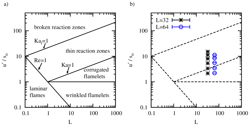
Figure 3.— Combustion Regimes Diagram. Part (a) shows a traditional turbulent combustion regime diagram (adapted from Peters (2000)) with regimes based on comparisons between the time scales, velocity scales and length scales of turbulence and a laminar flame. Part (b) shows the positions of the simulations on the regime diagram (blue circles and black asterisks) and the regime predictions (as dotted lines). Most of the simulations are predicted to be in the thin reaction zones regime.

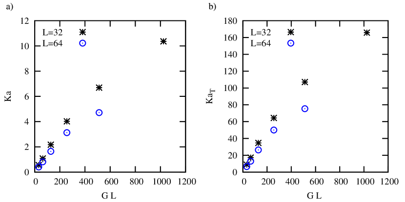
Figure 4.— Karlovitz Numbers. Part (a): the traditional Karlovitz number, $Ka=(\delta/\eta)^{2}$, measured from the simulations. Values over $1$ indicate that the simulation should be in the reaction zones regime. Part (b): the thermal Karlovitz number, $Ka_{T}=(4\delta/\eta)^{2}$, measured from the simulations. This is a Karlovitz number based on the laminar thermal width of the flame ($4\delta$). The large values of $Ka_{T}$ indicate that the viscous scale is much smaller than the thermal flame width for many of the simulations. The Rayleigh-Taylor instability is stronger for higher values of $GL$.

In order to check the validity of the regime diagram for RT unstable flames, it is first necessary to define the Karlovitz numbers for bistable model flames. These flames are thicker than more realistic model flames (e.g. the Arrhenius reaction) for which the reaction vanishes exponentially at low temperatures. The bistable reaction has a much less extreme drop-off at low temperatures, so the reaction is spread out over a larger physical space. The innermost reaction zone, where the reaction rate is fastest, is also larger for the bistable reaction than for the Arrhenius reaction. Nevertheless, to facilitate comparison with other simulations and experiments, we will use the standard definition of $Ka=(\delta/\eta)^{2}$ for most comparisons and define $Ka_{i}=(\delta_{i}/\eta)^{2}$ (assuming that $\delta=10\delta_{i}$), although these choices result in an underestimation of $Ka$ and $Ka_{i}$ for the bistable model flame. To remedy this difficulty, we also define a thermal Karlovitz number, based on the full thermal flame width $\delta_{T}=4\delta$ so $Ka_{T}=(4\delta/\eta)^{2}$. $Ka_{T}$ is an indicator of whether turbulent eddies are able to penetrate the physical flame width. Measurements of both $Ka$ and $Ka_{T}$ are shown in Figure 4. In addition, all of the simulations are shown on the regime diagram in Figure 3.

According to the regime diagram and the measured values of $Ka$, a few of the simulated flames should be in the corrugated flamelets regime, while most should be in the thin reaction zones regime. Specifically, for $L=32$, flames with $G\lesssim 2$ should be flamelets and for $L=64$, flames with $G\lesssim 1$ should be flamelets. For all higher values of $G$, the flames are expected to be in the reaction zones regime. Traditional turbulent combustion theory predicts that these flames should be thicker than the thermal laminar flame width (here, $\delta_{T}=4$) because eddies on scales smaller than the flame width should enhance thermal transport and thicken the flame.

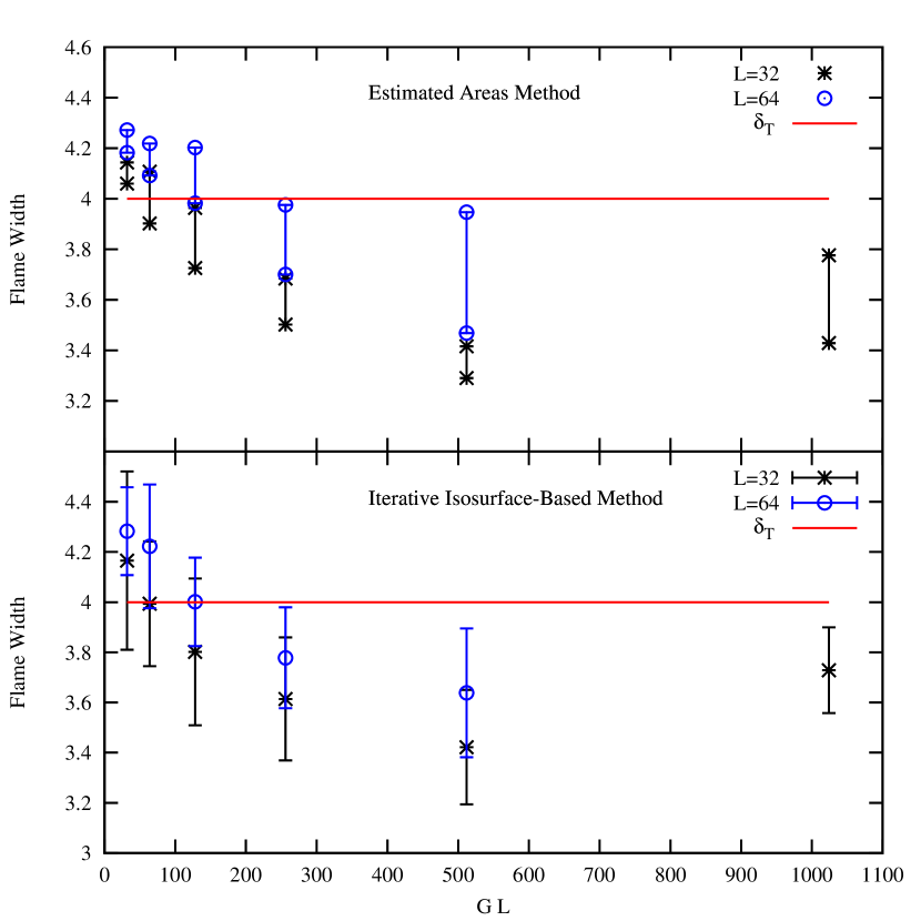
Figure 5.— Turbulent Thermal Flame Width vs. GL, calculated from the simulations by two different methods. Top Panel: Estimated Areas Method. Bottom Panel: Iterative Isosurface-Based Method; flame widths computed in post-processing. The laminar thermal flame width is $\delta_{T}=4$ and is indicated by a solid red line. Surprisingly, most of the simulations have a flame width smaller than the laminar thermal flame width, implying that although $Ka>1$ the flames are stretched flamelets instead of thin reaction zones.

To check this prediction, we measured the flame width in two different ways. Both methods involve dividing the flame volume by an area to estimate the flame width. In the first method, which we will call the “estimated areas method”, we measured the total volume of material between the $T=0.1$ and $T=0.9$ temperature contours and then divided that volume by two different indirect estimates of the flame surface area to find upper and lower estimates of the flame width. The first of these estimated areas is the flame surface area that would produce the measured turbulent flame speed if the turbulent flame speed follows the relation $s/s_{o}=A/A_{o}$, where $A$ is the area of the turbulent flame and $A_{o}$ is the area of the laminar flame. This assumption may overestimate the flame area, as discussed in Section IV.6, so this calculation gives a lower bound for the flame width. An upper limit for the flame width is calculated by assuming that the flame surface area is determined by the predicted Rayleigh-Taylor flame speed so $A=\sqrt{1+0.125GL}$. We calculated both lower and upper bounds on the flame width at each time step and then calculated the time-averaged bounds (excluding data from an initial transient period). The flame width range measured using this method is shown in the top panel of Figure 5.

The problem with dividing the entire flame volume by a representative surface area is that this area must be correctly chosen. In the estimated areas method, described above, we estimated these areas indirectly using physical reasoning. A more direct approach is to divide the isovolume by the surface area of a representative temperature contour, for example, the $T=0.5$ contour, but this requires choosing the “correct” contour. Different temperature contours can have very different surface areas, adding to the difficulty.

The second method, the “iterative isosurface-based method”, sidesteps these problems by using the surface areas of temperature isosurfaces to estimate the flame width iteratively. This method is described in detail and is mathematically formulated by Poludnenko & Oran (2010), see their Appendix A. The iterative isosurface-based method exploits the fact that isosurfaces with more similar $T$ values also have more similar surface areas. For instance, the $T=0.1$ isosurface area is much more similar to the $T=0.15$ isosurface area than to the $T=0.9$ isosurface area. This means that the flame width can be accurately estimated by dividing the total flame volume into smaller subvolumes bounded by isosurfaces defined by similar $T$ contours. Because these contours have similar surface areas, the average width of volume that they bound can be estimated unambiguously. Then, the average width of the entire flame is just the sum of the widths of the smaller flame subvolumes.

Ideally, the flame would be divided into infinitely many subvolumes, but in practice the number of divisions is limited by the resolution of the simulation. Subvolume widths should be close to, but not substantially less than, the resolution scale. This requirement suggests an algorithm in which the entire flame volume is divided into subvolumes, the width of each subvolume is calculated and then, if any subvolume width is greater than some factor, $\alpha$, of the resolution (Poludnenko & Oran (2010) used $\alpha=4$, we used $\alpha=2$), that subvolume is further divided iteratively. Poludnenko & Oran (2010) describe this algorithm in detail. We changed their algorithm in one way; Poludnenko & Oran (2010) used the area of the isosurface on only one side of the each subvolume to calculate the subvolume width. This is a reasonable procedure if the resolution of the simulation is small enough that the isosurface areas of the bounding $T$ contours are nearly identical. However, it is easy to calculate upper and lower bounds for the width of any subvolume by dividing the volume by the surface areas of both bounding isosurfaces. These bounds for the widths of the subvolumes are then added to get the total range of possible values for the total flame width.

We implemented the iterative isosurface-based method using the VisIt Python Interface (Childs, 2012). VisIt uses the marching cubes algorithm to construct contours and includes built-in queries for the isosurface areas and isovolumes. We ran our analysis code in post-processing, analyzing data files that were written out every tens to hundreds of time steps during the original simulations. Finally, we calculated a time-averaged flame width, using data from all the files except for those corresponding to the initial transient. The flame widths calculated using the iterative isosurface-based method are shown in the bottom panel of Figure 5.

The two flame width calculation methods (see Figure 5) produced similar results for the time-averaged flame width. Surprisingly, the flame is thinner at larger values of $GL$ instead of thicker as predicted by turbulent combustion theory. This implies that instead of being thickened by small-scale turbulent eddies, the flame is actually being thinned, probably by the stretching action of the Rayleigh-Taylor instability. The flames have not entered the thin reaction zones regime although $Ka>1$ and $Ka_{T}>>1$, instead they are stretched flamelets.

It is clear from these results that the traditional combustion regimes do not apply to RT unstable flames for the parameter values studied. Of course, it remains to been seen whether a transition to reaction zones occurs at higher $Ka$. It worth noting that even traditional turbulent flames often do not show a transition at $Ka=1$, although they may show a transition at higher $Ka$ (Driscoll, 2008). This suggests that the theory is only approximate, even for traditional turbulent flames. However, thinning of a flame is highly unusual and suggests that the inner structure of RT unstable flames is being determined by a straining mechanism (probably the RT instability) and that the flames are not being affected internally by small eddies. This fits with the physical picture of Rayleigh-Taylor unstable flames. Vorticity is created by temperature gradients across the flame front, and is not able to diffuse ahead of the flame (which has been confirmed by measurements in these simulations). If the vorticity is quickly driven downstream from the flame, the flame front will not interact with smaller turbulent eddies at all. Traditional turbulent combustion is geometrically and physically different because the flame moves through a turbulent fuel and is forced to interact with each individual turbulent eddy to propagate. RT flames do not have to interact with the turbulent eddies to propagate, so there is no reason to expect that they generally behave like turbulent flames. The observed thinning of the flame suggests that traditional turbulent combustion regimes do not apply to RT unstable flames and that, by proxy, flame speed models based on the physical ideas underlying the traditional turbulent combustion regimes also may not apply. We will directly compare some of these flame speed models to our results in the next section. Finally, these results imply that achieving DDT by transitioning to the reaction zones regimes may not be possible, since the transition may not ever occur.

IV. The Flame Speed and Comparison With Flame Speed Models

In this section, we will test the predictions of flame speed models using flame speed measurements from the parameter study simulations. Specifically, we will introduce and test several turbulence-based models and the RT-based model. Turbulence-based models generally give a dependence of the turbulent flame speed on the rms velocity ($u^{\prime}$) and other quantities. The models we will test include linear, scale invariant, and power law models. For each model we will compare the prediction of the model for the turbulent flame speed, $s$, in the entire domain with measurements. This procedure is not the most rigorous test of the subgrid models, which would involve implementing the models in simulations with unresolved scales, but it is a good basic check. Indeed, the scale at which the model is tested shouldn’t matter because all types of subgrid models currently in use are either compatible with the idea, or assume, that the flame surface is a fractal. The fractal nature of RT unstable flames was confirmed directly in 2D by Hicks & Rosner (2013).

Surprisingly, there is not one, universally-used definition of the turbulent flame speed, making it difficult to compare experimental and theoretical results in the field of turbulent combustion (Lipatnikov & Chomiak, 2002; Driscoll, 2008). It is even unclear whether there is one “correct” definition of the turbulent flame speed; different definitions may be more useful in different circumstances. In spite of these ambiguities, there is widespread agreement that the concept of a turbulent flame speed is still a useful one. There are at least two commonly used definitions of the global turbulent flame speed (Driscoll, 2008). The first definition, of the displacement speed, measures the physical distance covered by a certain isosurface of the flame in a certain time. This definition is isosurface dependent, and the calculated flame speed can depend by a factor of 2-3 on the isosurface chosen. The second definition, the global consumption speed, is based on the measurement of the total amount of fuel consumed by the flame in a given amount of time and the area of a chosen isosurface, so this measure is also isosurface dependent. In this paper, we use a third definition, the bulk burning rate (Vladimirova et al., 2003), which measures the global production of reactants per unit time, but does not rely on measuring isosurface areas. For our simulations, the bulk burning rate is defined as

$$s(t)=\frac{1}{L^{2}}\int_{0}^{L}\int_{0}^{L}\int_{-\infty}^{\infty}R(T)\,dydxdz.$$ (4)

The bulk burning rate is very similar to, but is less ambiguous than, the global consumption speed and is preferred when measuring the flame speed for model flames for which $R(T)$ is known. For the rest of this paper, we will refer to the bulk burning rate as the turbulent flame speed, $s$.

We will begin this section by giving a brief history and overview of models for the turbulent flame speed in Section IV.1 and then continue with a discussion of the specific turbulent flame speed models that have been implemented and used in full-star Type Ia simulations in Section IV.2. After a short explanation of how the measurements were made (in Section IV.3), we will compare the measurements of the turbulent flame speed to the predictions of several turbulent flame speed models in Section IV.4. Finally, in Section IV.5 we will compare the turbulent flame speed measurements with the predictions from the RT-based flame speed model.

IV.1. Turbulence Based Flame Speed Models: A History

Damköhler (1940, trans. 1947) was the first to make theoretical predictions of the turbulent flame speed and assess those predictions with experiments. By experimenting with Bunsen burner flames, he was able to identify two basic regimes of turbulent combustion by comparing the diameter of the Bunsen burner tube (which is the integral scale, $\ell$) and the width of the flame. If $\ell>\delta$, Damköhler found that the turbulent flame speed could be fit by the relation $s=A\,Re+B$, but if $\ell<\delta$ then $s\propto\sqrt{Re}$. In the modern language of flame regimes, $\ell>\delta$ corresponds to the flamelets regime and $\ell<\delta$ to the thin reaction zones regime. Theoretically, Damköhler considered the physical cause of these scaling laws. He reasoned that turbulence increased the surface area of the flame and, therefore, the flame speed, so that

$$\frac{s}{s_{o}}=\frac{A}{A_{o}}.$$ (5)

Considering the geometry of the Bunsen burner flame, Damköhler suggested that the wrinkling of the flame surface is proportional to $u^{\prime}$, so that for large values of $u^{\prime}$, $s/s_{o}\propto u^{\prime}$. Taking into account the requirement that the turbulent flame propagates at the laminar flame speed if $u^{\prime}=0$ this becomes

$$\frac{s}{s_{o}}=1+Cu^{\prime}$$ (6)

where C is a constant. This expression for the flame speed is still used today and fits many observations surprisingly well.

When $\ell<\delta$, in the thin reaction zones regime, Damköhler hypothesized that the smallest scale turbulence would not wrinkle the flame, but instead would enhance small-scale microscopic transport within the burning region. Then the turbulent flame speed is $s\approx(\kappa_{T}\alpha)^{1/2}$ where $\kappa_{T}$ is, in modern terms, the turbulent diffusivity and $\alpha$ is the reaction rate. This is the same as the equation for the laminar flame speed, $s\approx(\kappa\alpha)^{1/2}$, but $\kappa$ is replaced by $\kappa_{T}$. Then $s/s_{o}=(\kappa_{T}/\kappa)^{1/2}$ and finally

$$\frac{s}{s_{o}}\sim\left(\dfrac{u^{\prime}\ell}{s_{o}\delta}\right)^{1/2},$$ (7)

which reduces to $s/s_{o}\propto\sqrt{Re}$ if $Pr=1$. Summarizing, Damköhler’s predictions for the dependence of the turbulent flame speed on $u^{\prime}$ are $s\propto u^{\prime}$ if $\ell>\delta$ and $s\propto\sqrt{u^{\prime}}$ if $\ell<\delta$.

Since Damköhler’s time, there have a been many thousands of experimental measurements of the turbulent flame speed and tens of theoretical expressions formulated to explain the experimental results. A full history is beyond the scope of this paper; more information can be found in the many articles and textbooks that review the subject, for example see Bray (1980, 1990); Bradley (1992); Peters (2000); Lipatnikov & Chomiak (2002); Bilger et al. (2005); Law (2006); Driscoll (2008); Kuo & Acharya (2012); Lipatnikov (2013); Poinsot & Veynante (2013). We will only cover a few of the key points.

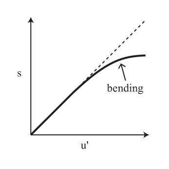
Figure 6.— The Bending Phenomena. This cartoon shows “bending” in the dependence of the turbulent flame speed, $s$, on the turbulent rms velocity, $u^{\prime}$. Bending refers to a deviation from linear dependence that results in a concave-down curve. This choice of axes is often referred to as a “burning velocity diagram”.

As experimental measurements of the flame speed were accumulated, a few basic properties of turbulent flames were noticed. First, the basic scaling $s\propto u^{\prime}$ generally fit the data well at low values of $u^{\prime}$, but at higher values of $u^{\prime}$ the linear dependence failed. The overall shape change from a straight line on a $s$ vs. $u^{\prime}$ plot (known as a burning velocity diagram) to a concave down curve at high values of $u^{\prime}$ is known as the “bending phenomena” (illustrated in Figure 6). It has been suggested that the bending behavior begins when the flame enters the thin reaction zones regime. Another clear experimental result is that there is not one “turbulent velocity scaling law” with fixed constants that fits all experiments. In fact, data points are widely scattered on the burning velocity diagram, with some experiments showing lots of bending and some showing none at all. Nevertheless, attempts were made to find a best average model by fitting the data aggregated from many experiments. Researchers have also compiled list of qualitative trends held in common by all or most experiments. After an analysis of a large number of experimental databases, Lipatnikov & Chomiak (2002) identified several basic trends, the first of which is an increase of $s$ with $u^{\prime}$ as $s\sim{u^{\prime}}^{q}$ with $q\approx 0.5$ being most likely (i.e. bending occurs for most flames). The other two basic trends are that $s$ and $ds/du^{\prime}$ are increased by $s_{o}$ and by pressure. Overall, it is clear that predicting the exact turbulent flame speed for an unknown system from first principles is exceedingly difficult.

Just as there have been many experimental measurements of the flame speed, there have been many theoretical models formulated to explain these experimental measurements. In general, many of these models are based on a set of physical assumptions about the way that turbulence should interact with flames, which, once combined, give an expression for $s$ in terms of $u^{\prime}$ and, often, other system parameters such as the integral scale and the laminar flame speed. Some examples of approaches include assessing the kinematic effect of turbulence on wrinkling directly (Damköhler, 1940, trans. 1947; Shchelkin, 1943; Clavin & Williams, 1979; Peters, 1999), modeling the flame as a fractal (Gouldin, 1987; Kerstein, 1988a), requiring the model to preserve scale invariance (Pocheau, 1992, 1994), considering random exchanges of state between burned and unburned cells (the pair-exchange model of Kerstein (1988b)), and modeling the interaction between turbulence and the flame as a series of vortex-flame interactions (Meneveau & Poinsot, 1991; Duclos et al., 1993). All of these approaches have been shown to produce acceptable fits to experimental data in some (but not all) cases. In certain regimes various models can be shown to be equivalent (Bray, 1990). A list of many of these models is given in Lipatnikov & Chomiak (2002), Appendix B and in Kuo & Acharya (2012), Table 5.1. Lipatnikov & Chomiak (2002) also compare various models to the experimental trends and highlight how well the models succeed (see their Table 2).

Currently, it is thought that a single, universal scaling law for $s(u^{\prime})$ that applies to all premixed turbulent flames across different combustion regimes probably does not exist. Factors like flame stretch, apparatus geometry, flame instabilities (such as the Landau-Darrieus instability), quenching and the details of the reaction chain may influence the turbulent flame speed. Because of these factors, a new focus has been to break premixed flames into categories by geometry and work to understand each category separately. Four common categories are envelope flames, oblique flames, flat flames and spherical flames (Driscoll, 2008). Unfortunately, none of these categories is a good fit for the geometry of Type Ia flames, so it is necessary to study Type Ia flames as a new category of premixed combustion. Direct study is necessary because the theory of premixed turbulent flames is not well-developed enough to predict scaling laws for new geometries from first principles. This is partially because it has not been possible to determine the “correct physics” by simply finding a working theoretical model since many models fit the data to some extent. A final complication is that the the bending phenomena is still not well-understood. Bending could be caused by a transition from flamelets to distributed burning, the merging and extinguishing of flamelets due to strain, gas expansion or geometrical effects (Driscoll, 2008). It is also possible that different causes of bending are in effect for different geometries. Overall, it is now clear that a single flame speed model, $s(u^{\prime})$, that is valid for all premixed turbulent flames is unlikely to exist.

IV.2. Astrophysical Flame Speed Models: History and Discussion

While it is clear that full-star Type Ia supernova simulations must incorporate a subgrid model, it is far from clear what that subgrid model should be. There have been three main attempts to adapt turbulent combustion theory for the Type Ia problem: a simple linear scaling law ($s=u^{\prime}$), a more complex LES treatment including a flame speed scaling law derived from considerations of scale invariance, and, finally, a flame speed scaling law meant to reproduce the bending seen in terrestrial flames. In this section, we will briefly discuss these models and distill their basic characteristics, which we will test against our simulations in Section IV.4. We will save a discussion of the RT-based subgrid model until Section IV.5.

In general, the choice of a subgrid model for Type Ia simulations is very difficult. First, geometrically there is no simple terrestrial analog from which a turbulent flame speed model might be taken. Consequently, there have been no terrestrial laboratory experiments which directly test ideas about Type Ia flames. Second, if the turbulent flame speed does depend on geometrical history (see Driscoll (2008)) then determining the turbulent flame speed from first principles could be almost impossible because conditions in the white dwarf and laminar flame properties change during the explosion process. Third, Type Ia flames are highly unstable to the Rayleigh-Taylor instability but the terrestrial flames from which the intuition of turbulent combustion has been developed are mostly either hydrodynamically stable, unstable to the Landau-Darrieus instability or unstable to various thermo-diffusive instabilities. Finally, the turbulence generated by the RT instability is downstream of the flame front and therefore probably affects the flame front differently than turbulence that is initially upstream of the flame front. In addition, it is likely that the turbulence generated by the RT instability is not homogeneous and isotropic, especially on large scales. All of these factors make adapting models from traditional turbulent combustion – which deals with a stable flame propagating through uniform turbulence – especially difficult.

Niemeyer & Hillebrandt (1995) first incorporated a turbulence-based subgrid model into Type Ia supernovae simulations by assuming a form for the turbulent flame speed at a given subgrid scale $\Delta$ of

$$s=s_{o}\left(\frac{u(\Delta)}{s_{o}}\right)^{n}$$ (8)

with $1/2\leq n\leq 1$ treated as a free parameter based on the value of the Gibson scale. For $n=1$, this result is equivalent to the classical Damköhler relation $s\approx u^{\prime}$ applied at the scale $\Delta$. Next, Schmidt et al. (2005, 2006a, 2006b) implemented a full LES (Large Eddy Simulation) model of turbulent energy evolution on unresolved scales based on a Germano decomposition filtering approach with localized eddy-viscosity and gradient-diffusion closures. In this approach, the turbulent flame speed at a given, unresolved scale $\Delta$ is derived from the subgrid-scale turbulent energy $k(\Delta)=(1/2){u^{\prime}(\Delta)}^{2}$ and the flame speed relation

$$\frac{s}{s_{o}}=\left[1+C_{t}\left(\frac{u^{\prime}(\Delta)}{s_{o}}\right)^{n}\right]^{1/n}$$ (9)

derived by Pocheau (1992, 1994). Here $n=2$ was chosen to enforce energy conservation, although this assumes that the turbulence has a Gaussian PDF, which is untrue for many turbulent flows (Pocheau, 1994). $C_{t}$ is a tunable parameter which was set equal to either $1$ or $4/3$ (see also Peters (1999)). This form of the turbulent flame speed equation is scale invariant in functional space which means that the interaction between the front geometry and the turbulent flow is scale invariant. Although scale invariance is a basic, if unstated, assumption of many turbulence-flame interaction models, most models violate this property. The scale invariant model is an inexact choice for Type Ia supernova flames because they are RT unstable and Equation (9) was derived for hydrodynamically stable flames in homogeneous and isotropic turbulence. Pocheau (1992, 1994) explicitly warns that the property of scale invariance may not hold for unstable flames. In terms of limiting behavior, Equation (9) reduces to $s\approx\sqrt{C_{t}}u^{\prime}$ when turbulence is strong, so this model does not produce the bending phenomenon, which is fundamentally not scale invariant. Numerically, the flame front is propagated by a level set method using the G-equation. The Schmidt model explicitly includes an approximation for the small-scale generation of buoyancy.

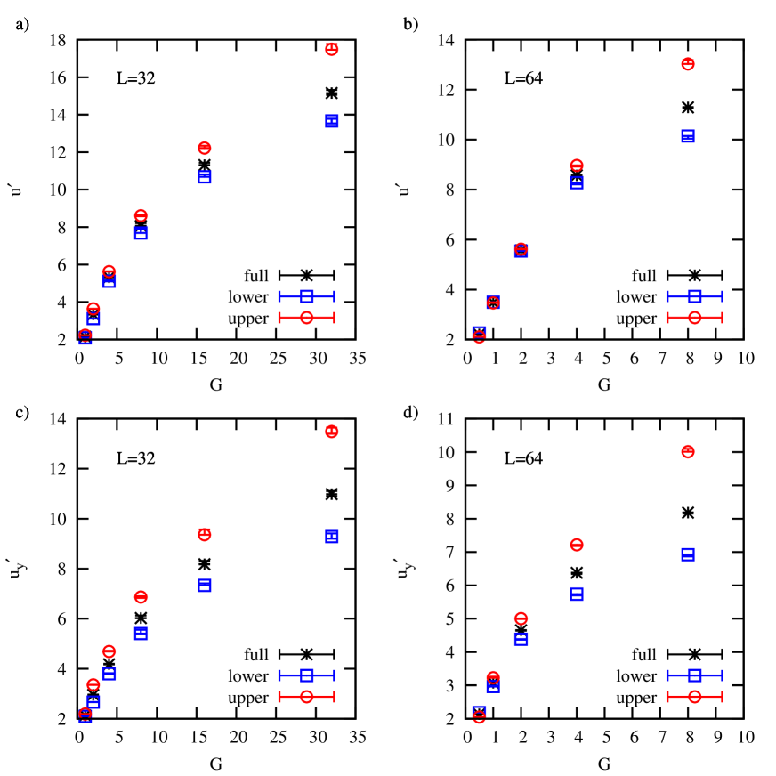
Figure 7.— Turbulent Velocities vs. $G$ for $L=32$ and $L=64$. These plots show $u^{\prime}$ and $u_{y}^{\prime}$ defined by averaging over three different spatial regions: the full flame brush (black asterisks), the top half of the flame brush (red circles), and the bottom half of the flame brush (blue squares). Of these three definitions, $u^{\prime}$ (and $u_{y}^{\prime}$) averaged over the full flame brush is the only truly global measure of the turbulent velocity. The other two measurements are shown as a general indication of the variation of $u^{\prime}$ with height. Generally, $u^{\prime}$ is larger in the upper half of the flame brush and the difference between the upper half and lower half $u^{\prime}$ measurements is larger at higher $G$. Averages were computed in post-processing.

Figure 8.— Flame Speeds, $L=32$. The turbulent flame speed, $s(t)$, as a function of time for the simulations with a domain width of $L=32$. The initial transient behavior is omitted from the plots and only the saturated oscillation of the flame speed around a stationary mean is shown. We calculate the average $s$ for each simulation from the data in these time intervals. Generally, the flame speed is larger and oscillates more wildly for higher values of $G$ at a fixed $L$.

Figure 9.— Flame Speeds, $L=64$. The turbulent flame speed, $s(t)$, as a function of time for the simulations with a domain width of $L=64$. The initial transient behavior is omitted from the plots and only the saturated oscillation of the flame speed around a stationary mean is shown. We calculate the average $s$ for each simulation from the data in these time intervals.

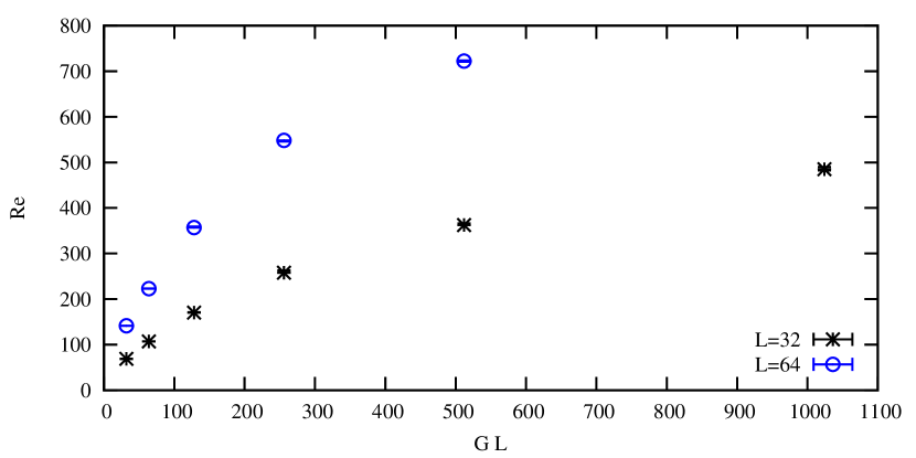
Figure 10.— Reynolds Number versus $GL$. The figure shows the Reynolds number based on the time-averaged $u^{\prime}$ for each simulation, so $Re=u^{\prime}L$ for $Pr=1$. The black asterisks represent the simulations with a domain width of $L=32$ and the blue circles represent simulations with a domain width of $L=64$. Each simulation is represented by one point on the plot. The product $GL$ is a basic measure of the strength of the Rayleigh-Taylor instability; larger $GL$ implies a stronger RT instability. The simulations range from laminar to moderately turbulent.

In contrast to the scale-invariant model implemented by Schmidt et al. (2005, 2006a, 2006b), Jackson et al. (2014) recently formulated an LES turbulence-flame interaction model specifically to account for bending at high turbulence levels. This model adapts an LES model for terrestrial flames (Colin et al., 2000; Charlette et al., 2002a, b)

$$\frac{s}{s_{o}}=\left(1+\frac{\Delta}{\eta_{c}}\right)^{\beta}$$ (10)

where $\eta_{c}$ is a cutoff scale for the wrinkling process and $\beta$ is a wrinkling exponent that could depend on scale. This model reduces to other models in various limits and can produce either the Damköhler scaling ($s\approx u^{\prime}$) or bending, depending on $\beta$ and on $\eta_{c}$. Physically, $\eta_{c}$ is the inverse mean curvature of the flame which depends on an efficiency function $\Gamma$ which, in turn, depends on the net straining of all scales below $\Delta$. This dependence is found by assuming a balance between flame surface creation due to wrinkling and destruction due to flame propagation and diffusion. In the model, $\Gamma$ is parameterized using the vortex-flame interaction measurements of Meneveau & Poinsot (1991). In other words, all interactions below the grid scale $\Delta$ are assumed to be equivalent to the summed action of vortex-flame interactions on all of those scales. This model can take quenching into account by enforcing the requirement that $\eta_{c}>\delta$. Numerically, flame propagation is achieved by the propagation of a thickened flame model. The current version of the model assumes that the turbulence is homogeneous and isotropic and does not take into account the effects of the Rayleigh-Taylor instability.

Although the two main LES models currently in use (Schmidt et al., 2005, 2006a, 2006b; Jackson et al., 2014) are relatively complex, they make fairly straightforward assumptions about the effects of turbulence on the flame. Both models assume that turbulence-flame interaction can be quantified using models adapted from terrestrial flame theory. These models either mostly or entirely ignore the effects of the Rayleigh-Taylor instability. The formulations of both models assume that the non-homogeneous and non-isotropic RT-generated turbulence downstream of the flame front interacts with the flame front in the same way as homogeneous and isotropic turbulence initially upstream of the flame surface would. In the next section, we will test the basic assumptions about the turbulent flame speed used in these models. Both models predict that the flame speed will either scale roughly as $s\approx u^{\prime}$ or as $s\approx{u^{\prime}}^{n}$ with $n<1$ to reproduce the bending behavior seen in terrestrial flame experiments.

IV.3. Flame Speed Measurements

In order to assess the various models for the turbulent flame speed, we measured both the turbulent flame speed, $s(t)$, using Equation (4) and the root-mean-square (rms) turbulent velocity, $u^{\prime}(t)$, for each simulation in the parameter study. The turbulent flame speed as a function of time for the $L=32$ and $L=64$ simulations is shown in Figures 8 and 9 respectively. The initial transient growth of the flame speed as the instability first develops is not shown. A few basic trends are apparent from the figures. First, the flame speed increases for larger $L$ or $G$ because flames with higher $GL$ are more unstable to the Rayleigh-Taylor instability and also generate more turbulence. Second, the size of the flame speed oscillations grows as $GL$ increases because the flame goes through more severe cycles of flame surface creation and destruction. For example, the flame speed for $L=32$, $G=1$ is constant because the flame surface is just a stable rising bubble, but the flame speed for $L=32$, $G=32$ is very oscillatory and complex because the flame is strongly deformed by the RT instability (see Figure 1).

For each simulation, we computed the average value of the flame speed, $s$, after excluding the initial transient, so that each point in $L$,$G$ parameter space is associated with one averaged value of $s$. It is this time-averaged value of $s$ that we compare to model predictions in the next section. To estimate the uncertainty associated with the averaging process, we calculated a running average error using the following procedure. For every point in the time series (excluding the initial transient), we computed the flame speed average using that point and all previous values of $s(t)$, so that as more data was added to the time series the computed averaged $s$ changed less. We considered the averaging “error” to be the range of averaged $s$-values computed as the last quarter of the time series points were added to the averaged data. This range of values is the uncertainty associated with averaging over a finite interval of an oscillating time series. In general, these errors are relatively small, which indicates that the times series are long enough to calculate a meaningful average. These error bars are shown in each plot.

In general, time-averaged quantities were calculated using the data written out at every time step during the simulation. However, some averages were calculated later, after the simulation was complete, using time snapshot data files which were written out on intervals of tens to hundreds of time steps. Averages computed using the data files alone are very close to averages computed at every time step. These averages are indicated as “computed in post-processing” in the relevant figures to distinguish them from averages computed at every time step.

An averaged turbulent rms velocity, $u^{\prime}$, was also computed for each simulation. In order to get a representative value of $u^{\prime}(t)$ at a given time, we used the formula

$$u^{\prime}(t)=\sqrt{<{u_{x}(t)}^{2}+{u_{y}(t)}^{2}+{u_{z}(t)}^{2}>}$$ (11)

where $<>$ indicates the spatial average over the volume between the top-most and bottom-most extent of the $T=0.5$ to $T=0.8$ contour range that also satisfies the criterion $T>0.5$. In other words, $u^{\prime}(t)$ is based on spatial averaging in the ashes.

Our definition of $u^{\prime}$ is clearly somewhat arbitrary: first, it depends on the selection of the temperature range $T=[0.5,0.8]$. However, measured values of $u^{\prime}$ do not depend strongly on the temperature interval selected; we repeated the calculation of $u^{\prime}$ using the interval $T=[0.1,0.9]$ and found similar results. Second, our definition of $u^{\prime}$ is based on averaging over the whole flame brush, which does not explore the variation of $u^{\prime}$ with height. This is in keeping with the goal of this section: to compare the global flame speed to flame speed models based on a global measurement of the turbulent velocity. But, although our global definition of $u^{\prime}$ is adequate for this purpose, the overall vertical variation of $u^{\prime}$ with height is still of great interest because RT unstable flames are expected to have much more vertical variation than turbulent flames. To give an idea of this variation, we show three different measurements of $u^{\prime}$ in parts (a) and (b) of Figure 7. The points represented by black asterisks show our measurements of $u^{\prime}$ averaged over the entire flame brush (this is the data that will be used for model comparisons throughout the rest of the section). Red circles show $u^{\prime}$ averaged only over the top half of the flame brush, and blue squares show $u^{\prime}$ averaged only over the bottom half of the flame brush. In general, $u^{\prime}$ is larger in the upper part of the flame brush than in the lower part. This difference is small at low $G$ and becomes significant at high $G$. In general, the variation of $u^{\prime}$ with height does not affect any of the qualitative conclusions in this paper. We plan to explore vertical profiles of flame data more thoroughly in a future paper.

We also calculated directional rms velocities using

$$u_{x}^{\prime}(t)=\sqrt{<{u_{x}(t)}^{2}>}$$ (12a)

$$u_{y}^{\prime}(t)=\sqrt{<{u_{y}(t)}^{2}>}$$ (12b)

$$u_{z}^{\prime}(t)=\sqrt{<{u_{z}(t)}^{2}>}$$ (12c)

Time-averaged values, $u^{\prime},u_{x}^{\prime},u_{y}^{\prime},u_{z}^{\prime}$ were calculated using the same time-averaging procedure and averaging error method as for the calculation of $s$. Measurements of $u_{y}^{\prime}$ are shown in parts (c) and (d) of Figure 7. The variation of $u_{y}^{\prime}$ with height does not affect the qualitative conclusions in this paper, except where noted. The Reynolds number for each simulation was calculated using $Re=u^{\prime}L/Pr$, in dimensionless variables. The Reynolds numbers for the simulations ranged between $70$ and $720$ showing that the simulations ranged from laminar to moderately turbulent, see Figure 10.

IV.4. Turbulence-Based Flame Speed Models Comparisons

In this section, we will compare our measurements of the time-average flame speed ($s$) and the time-averaged rms velocity ($u^{\prime}$) to various models. We consider three different basic types of models: simple linear models, scale invariant models and models that reproduce bending. As described previously, each of these classes of model represents a basic type of model used in traditional turbulent combustion theory and as subgrid models in astrophysical Type Ia simulations.

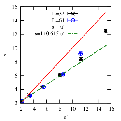
Figure 11.— Burning Velocity Diagram: Linear Models. The time-averaged turbulent flame speed ($s$) as a function of the time-averaged rms velocity ($u^{\prime}$) in the region downstream of the flame front. Data from each of the $L=32$ and $L=64$ simulations are shown as black asterisks and blue circles respectively. Error bars are based on the cumulative time averaging procedure discussed in Section IV.3 and represent the uncertainty associated with averaging over a finite oscillatory time series. Also shown are two simple linear model predictions. $s=u^{\prime}$ is shown as a solid red line and $s=1+Cu^{\prime}$ with a least-squares fit for the value of $C$, $C=0.615$ is shown as a dashed green line. Neither model is a good fit for the all of the data points.

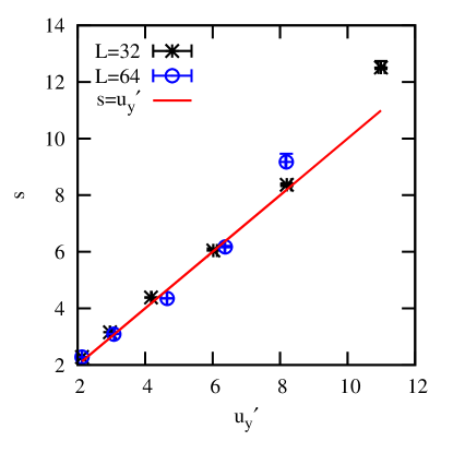
Figure 12.— Burning Velocity Diagram based on $u_{y}^{\prime}$. This figure shows a comparison between the measured time-averaged flame speed ($s$) and the rms velocity in the direction of flame propagation ($u_{y}^{\prime}$). $s=u_{y}^{\prime}$ (solid red line) fits the simulation measurements well for small values of $u_{y}^{\prime}$ (with no fitting parameter), but underestimates the flame speed for large values of $u_{y}^{\prime}$.

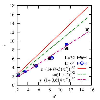
Figure 13.— Burning Velocity Diagram: Scale Invariant Models. This figure shows a comparison between measurements from the simulations (shown as black asterisks ($L=32$) and blue circles ($L=64$)) and the scale invariant flame speed model $s=(1+C_{t}{u^{\prime}}^{2})^{1/2}$, which is used as a subgrid model in many Type Ia simulations. The model with three different values of $C_{t}$ is shown: $C_{t}=4/3$ (the value used in the Type Ia simulations), $C_{t}=1$ (another value considered in the formulation of the subgrid model), and $C_{t}=0.614$ (a best fit to the simulation data). The two values associated with Type Ia subgrid models substantially overestimate the flame speed. The best fit model shows a pattern of residuals that indicates that it should not be extended to higher $u^{\prime}$.

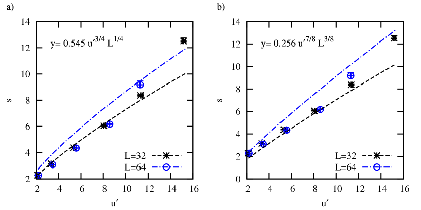
Figure 14.— Burning Velocity Diagram: Bending Models. These plots compare the simulation data ($L=32$, black asterisks; $L=64$, blue circles) and two models from traditional turbulent combustion theory: (a) the Zimont Model, $s=Cu^{\prime 3/4}L^{1/4}$ with best fit $C=0.545$ and (b) the Kerstein Pair Exchange Model, $s=C_{1}{u^{\prime}}^{7/8}L^{3/8}$ with best fit $C_{1}=0.256$. Both models depend on $L$ so two curves are shown for each model: the $L=32$ model curve is shown in black and should fit the black asterisk points; the $L=64$ model curve is shown in blue and should fit the blue circle points. Neither model adequately fits the data because the data are concave-up while the models are concave-down.

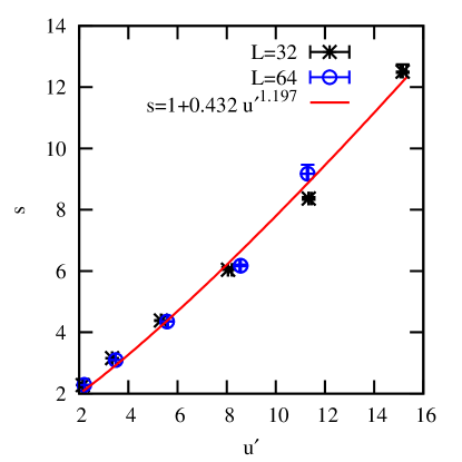
Figure 15.— Burning Velocity Diagram: Power Law Model. This plot compares the simulation data and a power law model $s=1+C{u^{\prime}}^{n}$ with a least-squares best fit of $C=0.432$ and $n=1.197$. This fit shows that the simulation data are concave-up ($n>1$), implying that Rayleigh-Taylor unstable flames are fundamentally different from traditional turbulent combustion flames, which show a linear or concave-down dependence ($n\leq 1$) on the same plot axes.

We first compare with our data with a simple linear model. The simplest and most obvious choice of all linear models is $s=u^{\prime}$, which is the high $u^{\prime}$ limit of the Damköhler law, Equation (6). A comparison between $s=u^{\prime}$ and the data from the simulations is shown in Figure 11 on a burning velocity diagram. The prediction $s=u^{\prime}$ is shown as a red line and the individual measurements from the simulations are shown as black asterisks ($L=32$ simulation data points) and blue circles ($L=64$ simulation data points). Each simulation is represented by one point on the plot. It is clear that the model $s=u^{\prime}$ overestimates the value of $s$. The second linear model is the full Damköhler law, $s=1+Cu^{\prime}$, with a fit for the value of C. The best least-squares fit for this law (with $C=0.615$) is show in Figure 11 as a dashed green line. The model line fits the data well for the smaller values of $u^{\prime}$, but underestimates the flame speed for larger values. The final linear model that we consider is $s=u_{y}^{\prime}$, which is shown in Figure 12. Interestingly, $s=u_{y}^{\prime}$ is a good fit for the data at low values of $u_{y}^{\prime}$ with no fitting parameter, although this is only true for $u_{y}^{\prime}$ defined by averaging over the entire flame brush; the actual value of $u_{y}^{\prime}$ varies considerably with height. The fact that $s=u_{y}^{\prime}$ fits the data well at low $u_{y}^{\prime}$ is consistent with the many models from traditional combustion theory in which the flame speed depends on the rms velocity in the streamwise direction only (the $y$-direction for these simulations). However, again, the model does not fit the data well for larger values of $u_{y}^{\prime}$: the flame speed grows faster than a linear function of $u_{y}^{\prime}$. Overall, linear models do not capture the overall trend of the data in the $s$-$u^{\prime}$ plane.

Second, we compare the data with scale invariant flame speed models of the type $s=(1+C_{t}{u^{\prime}}^{2})^{1/2}$. This is the flame speed model used by Schmidt et al. (2005, 2006a, 2006b) as a subgrid model for full-star Type Ia simulations. Figure 13 shows a comparison between this model and the simulation measurements for the two values of $C_{t}$ used by Schmidt et al. (2005, 2006a, 2006b), $C_{t}=4/3$ (solid red line) and $C_{t}=1$ (dashed green line). It is clear that both of these models substantially overestimate the actual flame speed and that this overestimation is worse for intermediate values of $u^{\prime}$ and then improves slightly for large values of $u^{\prime}$. In practice, this means that Type Ia simulations using this subgrid model may be substantially overestimating subgrid deflagration speeds. This is not surprising because there is no particular physical reason to expect that $C_{t}$ should be $1$ or $4/3$. In fact, Schmidt et al. (2006b) suggested that $C_{t}$ should be a fitted parameter. Following this suggestion, Figure 13 also shows the least-squares best fit which is $C_{t}=0.614$ (purple line). This result fits the data well, but an examination of the residuals shows that the model consistently underestimates the flame speed at low values of $u^{\prime}$, overestimates it at intermediate $u^{\prime}$, and underestimates it at high $u^{\prime}$. Because of this clear pattern, which is the result of fitting an almost straight line to a curved data set, we have no confidence in an extension of this best fit model to higher values of $u^{\prime}$. Overall, scale-invariant flame speed models do not fit the simulation measurements well; in addition, the values of $C_{t}$ used in Type Ia subgrid models significantly overestimate the flame speed.

Finally, we compare the simulation results to two models that reproduce the bending phenomena seen in terrestrial flames. The Type Ia subgrid model used by Jackson et al. (2014) is also meant to reproduce bending, but we will not test that model directly because of its more difficult formulation. To check whether models that reproduce bending fit the data well, we consider two of the models shown by Lipatnikov & Chomiak (2002) to best fit the terrestrial flame experiments: the Kerstein pair-exchange model (Kerstein, 1988b) and the Zimont model (Zimont, 1979; Zimont et al., 1998). Both models reproduce the bending behavior and both have a fittable parameter. We consider them as general representatives of models that produce the bending and thereby test the Jackson model implicitly. The Zimont model is based on kinematic wrinkling of the flame by large eddies and thickening of the flame by small scale eddies and is given by $s=Cu^{\prime}Da^{1/4}$ or $s=Cu^{\prime 3/4}L^{1/4}$ using $s_{o}=1$. Figure 14, part (a) compares this model with the simulation data. The Kerstein pair-exchange relation models the propagation of flamelets as a random exchange of the burned and unburned states of fluid elements in the streamwise direction. Using standard turbulence scalings, the turbulent flame speed is then given by $s=C\sqrt{s_{o}u^{\prime}}Re^{3/8}$, which is equivalent to $s=C_{1}{u^{\prime}}^{7/8}L^{3/8}$, using $s_{o}=1$. A comparison of this model with the simulation data is shown in Figure 14, part (b). It is clear that neither model in Figure 14 fits the data well. Fitting the low $u^{\prime}$ data well inevitably results in the flame speed for the simulation $G=32$,$L=32$ being significantly underestimated. In addition, the dependence on $L$ is problematic for both models because $L$ doesn’t affect the flame speed at low values of $GL$. Overall, the problem is basically the same as with the linear models – the data are concave-up, while models that reproduce bending are concave-down. No model that produces concave-down bending, including these representative models and the Jackson et al. (2014) model, will fit our concave-up data.

Overall, tests of linear models, scale invariant models and bending models show that none of these models can successfully fit the data from our simulations. The fundamental issue is that none of these models fits the shape of the data on the burning velocity diagram. In Figure 15, we show that the best fit of $s=1+C{u^{\prime}}^{n}$ is $n=1.197$; our data curve is concave-up, not linear (like the linear or scale invariant models at high $u^{\prime}$) or concave-down (like the bending models). This concave-up dependence of $s$ on $u^{\prime}$ is different from the concave-down dependence of typical turbulent flames. This suggests that Rayleigh-Taylor unstable flames behave in a completely different way from flames moving through an upstream field of turbulence. We have shown that it is inappropriate use flame speed models from traditional turbulent combustion theory for RT-unstable flames.

IV.5. Rayleigh-Taylor Flame Speed Model Comparison

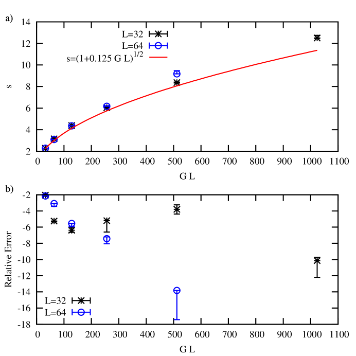
Figure 16.— Rayleigh-Taylor Flame Speed Model compared with the simulation data. Part (a) shows a direct comparison between the RT flame speed model prediction (solid red line) and the time-averaged flame speeds measured from the simulations (black asterisks for $L=32$, blue circles for $L=64$). Part (b) shows the relative error (RE) between the predicted value (PV) and the simulation data (SD), defined as RE=100*(PV-SD)/PV. The error bars in both plots represent the uncertainty of averaging over a finite-time oscillating time series (see Section IV.3).

The Rayleigh-Taylor subgrid model was first suggested by Khokhlov (1995) and then expanded by Zhang et al. (2007). In the RT model, the flame speed is determined by a balance between flame surface creation by the instability and destruction by geometrical effects. The geometrical destruction rate is set by the rate of collisions between flame sheets, which is determined by the volume of the Rayleigh-Taylor bubble. In this model, the RT instability sets the flame speed because it controls the rates of both flame surface creation and destruction. The flame speed relation itself can be derived from dimensional analysis, from the linear growth rate of the RT instability, or from the speed of a rising buoyant bubble. The expected flame speed is then, in our dimensionless units, $s=s_{o}\sqrt{0.125GL}$, for large $GL$ (Khokhlov, 1995). Because $G$ depends on $1/s_{o}^{2}$, this result implies that the turbulent flame speed should be independent of the laminar flame speed. Zhang et al. (2007) showed that this is the case for a carbon-oxygen flame.

There have been several tests of the flame speed relation, both in 2D and in 3D. In 2D, Vladimirova & Rosner (2003, 2005) confirmed the predicted RT scaling up to $GL=128$ for reflecting boundary conditions, and $GL=512$ for periodic boundary conditions. They corrected Khokhlov’s prediction at low values of $GL$, finding $s=s_{o}\sqrt{1+0.0486(G-G_{1})L}$ where $G_{1}=8(2\pi/L)^{1.72}$ is the transition point between planar and cusped flames. This correction ensures that the flame will move at the laminar flame speed, $s_{o}$, when the $GL=0$. At high $GL$, this is equivalent to Khokhlov’s prediction, but with a different constant because the measurements were carried out in 2D. In a previous paper (Hicks & Rosner, 2013), these simulations were extended to $GL=16,384$ and a best fit scaling of $s=s_{o}\sqrt{1+0.0503(G-G_{1})L}$ was found, which is consistent with the Rayleigh-Taylor model. All of these 2D tests were direct numerical simulations designed to resolve both the flame width and the viscous scale. Zhang et al. (2007) carried out three-dimensional tests of the Rayleigh-Taylor model and confirmed the RT scaling to within $10\%$ for $GL=400,671,1493,2786$. However, these calculations did not fully resolve all scales, and, in particular, were unable to resolve the Gibson scale even at their highest resolution. An additional problem is that their averages included very few flame speed oscillations. In general, past studies of RT-unstable flames have shown that their flame speeds are consistent with the RT model in both 2D and in 3D, but the 3D tests had some drawbacks.

Our 3D simulations are similar in some ways to Zhang et al. (2007), but they are fully resolved down to the viscous scale and the average flame speed is computed from many more flame oscillation periods (compare Figures 8 and 9 with Zhang et al. (2007), Figure 20). We also checked the scaling law over a large total range in $GL$, from $GL=32$ up to $GL=1024$. Figure 16, part (a) shows a comparison between our results and the 3D RT-predicted flame speed (with the correction to account for the laminar flame behavior), $s=s_{o}\sqrt{1+0.125GL}$. The time-averaged flame speed is shown as black asterisks for simulations with a domain width of $L=32$ and blue circles for $L=64$; the RT prediction is shown as a red line. For low values of $GL$, the RT prediction matches the data well but a deviation of around $14\%$ is seen for the $L=64$, $GL=512$ case. The $L=32$, $GL=1024$ case shows a deviation of around $10\%$. The relative error between the predictions and the simulation data results are shown in Figure 16, part (b). In this plot, the error bars based on the uncertainty of averaging over the oscillating flame speed can be clearly seen. These uncertainties are not large enough to account for the deviation from the Rayleigh-Taylor model. There are also other uncertainties, but we have been unable to find one large enough to account for the difference between the RT prediction and the data. In addition, there seems to be a difference between the $L=32$ and $L=64$ simulation flame speeds at $GL=512$ implying that there could be a domain-size dependence that is not accounted for in the RT flame speed model (which depends only on the product $GL$). So, while the RT flame speed model predicts the flame speed well at low $GL$, at higher $GL$ the turbulent flame speed is larger than predicted. In the next section, we will discuss a physical mechanism that could explain these higher than predicted flame speeds.

IV.6. Cusps – The Missing Ingredient?

In the previous section, we showed that our simulated flame moves faster than the RT flame speed for higher values of $GL$. In this section, we will discuss a mechanism that could produce these higher than expected flame speeds – the formation of cusps, either by turbulence or by the Rayleigh-Taylor instability. After giving a geometrical definition of two different types of cusps, we will discuss three cusp formation mechanisms and the three different local flame speeds associated with cusps. Next, we will review results from Poludnenko & Oran (2011) that explain how a local increase in the flame speed can induce a faster global turbulent flame speed. Then we will compare two simulations that the RT model predicts should have the same flame speed, but don’t, and discuss circumstantial evidence in favor of one of the simulations being more affected by cusps than the other. Finally, we will consider possible measurements that could further clarify the role of cusps.

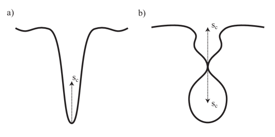
Figure 17.— Cusps: Local and Nonlocal. Part (a) shows a local cusp: a locally-formed region of high curvature that propagates with a phase speed $s_{c}$. Local cusps can be formed by the Huygens mechanism, turbulence or the Rayleigh-Taylor instability. Part (b) shows two nonlocal cusps that formed when two initially distant sections of the flame surface were pushed together, either by turbulence or by the RT instability. This figure is based on Figure 11 of Poludnenko & Oran (2011).

Figure 18.— Cusp formation by the Huygens mechanism. At time $t_{1}$ the flame is perturbed into a sinusoidal shape by an instability. At every point along the flame surface, the flame propagates normal to itself at the laminar flame speed. At time $t_{2}$ this normal propagation has enhanced the peaks of the flame surface, but is beginning to destroy the valleys. By time $t_{3}$ the valleys have been completely destroyed, leaving local cusps in their place. Now, the local normal propagation of the flame front reinforces the cusp shape – it is stable as long as the peaks are not too high. This figure is based on Figure 1 from Zel’dovich (1966).

A flame surface cusp (or “corner”) is a part of the flame surface area where the radius of curvature of the surface is very high (see Figure 17). This gives the flame surface the appearance of a rounded v-shape with the angle between the sides of the v being small so that the two flame sheets that comprise the sides of the v approach nearly head-on. Khokhlov (1995); Poludnenko & Oran (2011) have identified two different types of cusps. A “local” cusp is one that forms when a spatially-local section of a flame is deformed into a cusp shape (see Figure 17, part (a)). Two “nonlocal” cusps form when two parametrically-distant sections of the flame surface meet at a low angle of incidence, forming two cusps on either side of the point of contact point (see Figure 17, part (b)). Once formed, local and nonlocal cusps behave in the same way; however, their different formation mechanisms influence their prevalence in a given flow.

A variety of physical mechanisms can trigger the formation of local and nonlocal cusps: formation due to the normal-directional propagation of a perturbed flame surface (the Huygens mechanism), due to turbulence or due to the Rayleigh-Taylor instability. Huygens cusp formation, illustrated in Figure 18 occurs when a flat flame surface is slightly disturbed by a perturbation that creates “peaks” and “valleys” on the flame surface. Generally, each section of the flame surface propagates normally to itself at the laminar flame speed, according to the Huygens principle. Flame surfaces in the valleys meet, effectively creating cusps, while flame surfaces near the peaks diverge, enhancing the peak. The final flame surface is a series of alternating peaks and local cusps. Zel’dovich (1966) first proposed this cusp formation mechanism and that the formation of these cusps could stabilize the Landau-Darrieus instability of the flame surface. Stabilization of this sort is not particular to the LD instability, but can also occur for flame surfaces perturbed by the RT instability or by turbulence.

A second method of cusp formation, formation of cusps by turbulence, is extensively discussed in Khokhlov (1995); Poludnenko & Oran (2011). Turbulence can form both the local and nonlocal cusps already mentioned. A local cusp forms when the turbulent eddies fold the flame into a cusp shape, with the vertical extent of the “v” being roughly the size of the eddies. Nonlocal cusps form when large-scale turbulent motions fold the flame surface, pushing together sections of the flame sheet.

For Rayleigh-Taylor unstable flames, we identify another mechanism of both local and nonlocal cusp formation – formation of cusps due to Rayleigh-Taylor fingering. As the RT instability acts on the flame surface it produces “fingers” of unburnt fuel that penetrate into the burned ashes. These fingers consist of a long tube of fluid connected to a mushroom-shaped head (see Figures 19 and 20). The evolution of any individual finger creates both local and nonlocal cusps. The 2D cartoon (Figure 19), shows two local cusps on either side of the mushroom head. As the flame consumes the finger of fuel, the two flame sheets that make up either side of the tube (in 2D) will eventually come into contact forming nonlocal cusps. In the actual 3D simulations (Figure 20), the local cusp is a ring that wraps around the mushroom head and the nonlocal cusps are complex structures created when parts of the tube come into contact. For each RT finger at least one ring-like local cusp and two or more complex non-local cusps form. Rising bubbles of ash can also form local cusps as they rise. Of course, this mechanism is not entirely independent of the turbulent cusp formation mechanism, because local flows around the RT fingers do influence their formation and evolution.

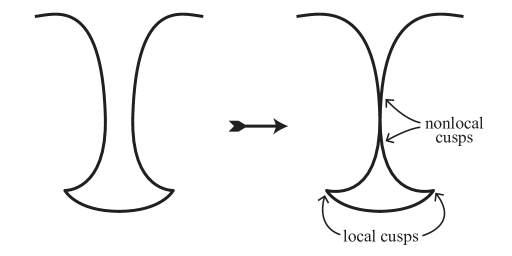
Figure 19.— Cusp Formation by the Rayleigh-Taylor Instability. This cartoon shows how the evolution of a Rayleigh-Taylor finger generates both local and nonlocal cusps. As the finger evolves, the formation of the mushroom-like head generates two local cusps (in 2D, as shown in the cartoon), or a ring local cusp (in 3D). As the fuel in the finger is burned, the sides of the finger approach each other and contact, forming two nonlocal cusps.

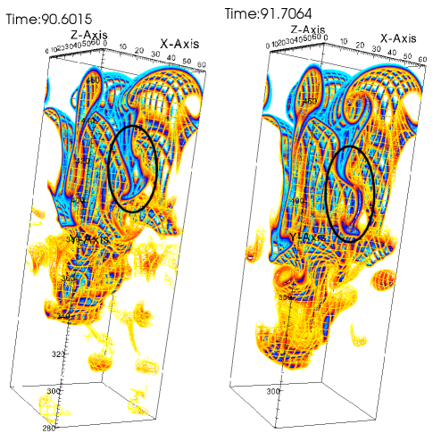
Figure 20.— Cusp Evolution. This contour plot of temperature shows the evolution of several RT-generated cusps in the simulation $L=64$, $G=8$. The left side of the figure shows a RT fuel finger (circled in black) penetrating into the burned ashes region. The right side of the figure shows the same finger about one flame-crossing time later. The tube part of the finger has pinched, forming two nonlocal cusps. In addition, the local cusp in the mushroom part of the finger has evolved, becoming sharper. Note that several other cusps can also be seen evolving in the figure.

There are three basic burning speeds associated with each cusp that forms: the local laminar flame speed ($s_{o}$), the cusp phase speed ($s_{c}$) and the local cusp burning speed ($s_{n}$); each of these speeds is discussed in detail by Poludnenko & Oran (2011). Parts of the flame far from regions of high curvature propagate at the laminar flame speed. The cusp itself travels at the cusp phase velocity. This speed is set by the geometry of the collisions between the flame sheets that make up the sides of the cusp and does not represent a physical consumption of fuel. The smaller the angle ($\alpha$) between the two sheets, the faster that the cusp will propagate because $s_{c}=s_{o}/sin(\alpha)$ (see Figure 21). This speed can be very large, and has been measured to be as high as $s_{c}=55s_{o}$ for cusps studied by Poludnenko & Oran (2011) and as high as $s_{c}\approx 10s_{o}$ for the Bunsen burner flames studied by Poinsot et al. (1992). Thus, cusps can disappear very rapidly after forming. The third basic burning speed is the local cusp burning speed, $s_{n}$. This speed is a magnification of fuel consumption in the cusp and is due to the geometrical focusing of thermal diffusion in the region where the flame sheets are very close together (Poludnenko & Oran, 2011). This speed, which has its maximum, $s_{n}^{*}$, at the point of highest curvature, depends on $\alpha$; the focusing effect is stronger at smaller angles. Poludnenko & Oran (2011) measure $s_{n}^{*}\approx 1.2s_{o}$ when $\alpha=4\degree$ and $s_{n}^{*}\approx 3.2s_{o}$ when $\alpha=1\degree$ (see their Figure 14, part (b)). Clearly, $\alpha$ must be very small to significantly enhance the local cusp burning speed, but these amplifications can be significant. The increase should be larger in 3D than in 2D. Of the three burning speeds of the cusp, only the local cusp burning speed reflects an actual increase in fuel consumption.

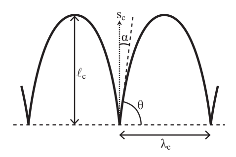
Figure 21.— Cusp Angles and Lengths. This diagrams shows various dimensions and angles associated with a cusp. $\alpha$ spans half of the opening angle of the cusp, $\ell_{c}$ is the amplitude of the cusp and $\lambda_{c}$ is the wavelength of the cusp.

The local cusp burning speed indicates whether the flame fuel consumption is enhanced locally, but it doesn’t quantify the extent to which the global flame speed will be amplified. Clearly, the extra fuel consumption in the cusps will only have a large influence on the total global fuel consumption if cusps are prevalent on the flame surface. Poludnenko & Oran (2011) quantify this by showing the total global flame speed enhancement caused by 2D cusps as a function of the total length of the cusp, $l_{c}$, divided by the laminar flame width, $\delta$, for various values of $\alpha$ (see their Figure 15). To summarize their result, global flame speed enhancements of $10\%$ are possible for $\alpha=1\degree$ for $l_{c}/\delta\approx 15$ and for $\alpha=2\degree$ for $l_{c}/\delta\approx 5$. While these results can not be used to directly test whether the flame speed enhancements observed in our simulations are due to cusp burning, it is possible to check the basic order of magnitude for plausibility. If we assume that the RT-unstable flames in our simulations would have a flame speed equal to the RT flame speed predicted value without the extra fuel consumption of the cusps, then the $L=64,G=8$ simulation has approximately a $14\%$ flame speed enhancement due to cusps and the $L=32,G=32$ simulation has a $10\%$ enhancement due to cusps (see the model errors in Figure 16). Assuming an $\alpha$ for the cusps of a few degrees, which seems plausible because many of the cusps are non-local collisions, then if $l_{c}$ is relatively small these numbers are roughly of the same order as the flame speed enhancements predicted by Poludnenko & Oran (2011). A larger $l_{c}$ than those discussed by Poludnenko & Oran (2011) should produce the flame speed enhancements measured for our simulations because larger fuel consumption amplifications are expected for 3D cusps. Overall, the theory that burning in cusps could increase the flame speed approximately $10-15\%$ above the RT flame speed seems plausible based on these estimates.

Another plausibility check for the hypothesis that cusps can enhance the flame speed is to compare two simulations that should have the same flame speed according to either the RT or turbulence-based models yet do not. In particular, we compare $L=32,G=16$ (Simulation A) and $L=64,G=8$ (Simulation B). The RT flame speed model predicts a flame speed of $s=8.06$ for both simulations because they each have $GL=512$. Turbulence-based models based on $u^{\prime}$ alone also predict the same flame speed for both simulations because they have very similar measured values of $u^{\prime}_{A}=11.33$ and $u^{\prime}_{B}=11.29$ (the $u_{y}^{\prime}$ values are also similar). In spite of these similarities, Simulations A and B have significantly different flame speeds: $s_{A}=8.37$ and $s_{B}=9.18$. We will examine A and B more closely to try to determine why their flame speeds are so different and whether this difference is due to cusps.

To begin, we check the flames visually for the presence of cusps. Overall, B (Figure 2, $G=8$) has more complex cusp structures than A (Figure 1, $G=16$). Simulation A does have cusps, but they tend to be single, large cusps instead of the many smaller cusps in Simulation B. $L=32$, $G=32$ also has many, smaller cusps which may explain its enhanced flame speed. Next, we compare the flame heights of the simulations to infer the likely geometry of the flame. We define the flame height at any given time ($h(t)$) as the distance between the top and bottom-most positions of any contour between $T=0.5$ and $T=0.8$. Physically, the flame height is a measure of the vertical extent of the flame. We averaged over time to find the average flame height, $h$, for each simulation. We found that $h_{A}/L=2.84$ but $h_{B}/L=2.57$, so the flame in B is, on-average, more compact vertically than the flame in A suggesting that B has shorter cusps than A. Shorter cusps are consistent with a higher surface density of cusps because more cusps per surface area means that each cusp gets less fuel and doesn’t sink as far before it is burned. Both a visual inspection of A and B and a comparison of their flame heights support the hypothesis that cusps are causing flame speed enhancements in B.

But do these cusps form mostly due to turbulence or due to the RT instability? It is hard to know for certain, but there are two pieces of indirect evidence that favor the dominance of RT cusps. First, visual inspection of the flame shows that the cusps resemble evolving RT fingers. Second, if turbulence were causing most cusp formation, simulation A should be more affected by these cusps than B because its Karlovitz number is higher (see Figure 4). A larger $Ka$ implies that the velocity at the scale of the flame width is larger for A than for B, so A should form local turbulent cusps more effectively than B. The fact that the opposite is true – B seems to be more affected by cusps than A – implies that the cusps are mostly not local cusps formed by turbulence. Overall, the evidence favors the cusps being formed by the RT instability.

In this section, we reviewed and applied past work on the enhancement of the global flame speed by cusps to our simulations of RT unstable flames. Cusps increase the local rate of fuel consumption; the net global effect is a flame that moves faster than expected from its surface area alone. Our basic hypothesis is that, without cusps, the flame would move at the RT-predicted flame speed. We suggest that any “extra” flame speed is due to the enhancement of the local burning velocity by cusps. If cusps are prevalent, then these local enhancements can increase the global flame speed. To evaluate the plausibility of this argument, we first compared the size of the speed enhancements from our simulations to predictions from Poludnenko & Oran (2011) and found that the $10-15\%$ enhancements that we observe are not too large to be generated by cusps. Second, we compared two simulations with different flame speeds that were predicted to have the same flame speed by both RT and turbulence-based flame speed models. The faster of these flames visually seems to have more cusps than the slower flame. In addition, it has a shorter normalized flame height, implying that fuel is being directed into many shorter cusps instead of fewer longer cusps. Finally, we argued that the cusps are more likely to have been formed by the RT instability than by turbulence. A true understanding of the role of cusps in RT unstable flames can only be achieved by further research. In particular, it may be possible to directly measure the contribution of cusps by comparing the surface area of a selected contour of the flame surface to the flame speed. Poludnenko & Oran (2011) used this procedure to study turbulent flames and showed that the flame could travel faster than accounted for by its surface area. They suggested that the excess flame speed was due to speed amplification by cusps. A similar analysis could be attempted for RT unstable flames. Moreover, direct study of the types of cusps formed by RT unstable flames, especially when paired with a cusp detection algorithm could allow for direct measurements of cusps and detailed quantification of their effect on the flame speed.

V. Discussion and Conclusions

In this paper, we explored the physics of RT unstable flames and considered the effects of the RT instability and the turbulence generated by the instability on the flame front. In particular, we considered two different types of turbulent flame speed models – turbulence or RT based – and assessed their physical appropriateness and ability to fit our flame speed data. Turbulence based flame speed models are based on traditional turbulent combustion theory, but can this theory make successful predictions about RT unstable flames? Does turbulence have the same effect whether it is upstream or downstream of the flame front? Can turbulence downstream of the flame front overwhelm the RT stretching of the flame and set the flame speed? The answers to these questions are necessary to determine whether subgrid models based on traditional combustion theory should be used in Type Ia supernovae full-star simulations. We attempted provide them in two different ways: first, we checked whether the flame followed the traditional turbulent combustion regimes; second, we checked the predictions of several types of turbulence-based model and the RT-based model. We simulated 11 different parameter combinations of $G$ and $L$ in order to probe the full range of flame behavior from simple to complex. To test predictions, we calculated the average flame width, the average flame speed, the average flame height and the average rms velocity of the turbulence behind the flame for each simulation.

To begin, we tested a basic prediction of traditional turbulent combustion theory: the flame should transition from flamelets to reaction zones at $Ka=1$ and thicken when $Ka>1$. Because most of the simulations should be in the thin reaction zones regime based on their Karlovitz number, we expected to find that the flames were thickened by eddies smaller than the flame width. In fact, we found just the opposite; in general, the flames were thinner than the laminar flame width. This suggests that the traditional picture of viscous eddies thickening the flame front does not hold for RT unstable flames. On the contrary, the thinning of the flame by RT stretching seems to overwhelm turbulent thickening. If the vorticity generated by the flame front is rapidly washed downstream, it will not have the opportunity to interact with the flame front and thicken it. Then RT stretching will be the main influence on the flame front, which will be thinner than expected. In summary, we found that the flame did not undergo a basic regime change predicted by traditional turbulent combustion theory and, therefore, that flame speed predictions based on this theory must be suspect. There is another implication of the failure to find the transition at $Ka=1$: the reduced plausibility of the Zel’dovich gradient mechanism for DDT for these flames. The Zel’dovich gradient mechanism for the DDT specifically depends on a large specially conditioned reactivity gradient being established in the white dwarf. It has been generally assumed that this gradient is produced by the thickening of the flame as it transitions into the reaction zones regime. However, the fact that we have been unable to find such a transition for RT unstable flames casts doubt on this assumption. An important question is whether the flame will actually undergo the transition and thicken if the turbulence is stronger than in these simulations; this is an important avenue for future research.

The second test of whether traditional turbulent combustion theory can predict the behavior of RT unstable flames was to compare its flame speed predictions with measurements from simulations. We tested three basic flame speed predictions: linear, scale invariant, and power law models. All three types of model have been used as subgrid models for full-star Type Ia supernovae simulations. Of the three linear models tested, $s=u^{\prime}$ substantially overestimated the flame speed, and $s=1+Cu^{\prime}$ and $s=u_{y}^{\prime}$ underestimated the flame speed at high $u^{\prime}$. It is worth noting that $s=u_{y}^{\prime}$ did fit the data well at lower values of $u^{\prime}$ without any sort of fitting constant, although this may be due to “lucky averaging” over the variation of $u_{y}^{\prime}$ with height. Next, we tested the scale invariant model given by Equation (9) and showed that the commonly used values of $C_{t}=4/3$ and $C_{t}=1$ substantially overestimate the flame speed. This suggests that the many full-star simulations using this subgrid model have flames that propagate too quickly. In addition, we pointed out that the scale invariant model is not physically appropriate for a RT unstable flame, since its formulation is only valid for hydrodynamically stable flames. Finally, we tested models meant to reproduce the “bending phenomena” seen in terrestrial flames at higher values of $u^{\prime}$. This sort of model has been recently adapted by Jackson et al. (2014) for astrophysical flames. These models fail to fit our data, because the flame starts to move relatively faster at high values of $u^{\prime}$ instead of slower. In other words, our flame speed data do bend, but they bend up instead of down. The fact that the flame speed curve is concave-up on the burning-velocity diagram shows why none of the models adapted from traditional turbulent combustion theory work – all of those models are either linear, nearly linear or concave-down. RT unstable flames behave in a very different way from typical turbulent flames, especially when the turbulence is strong. This suggests that the practice of assuming that flame speed models from traditional turbulent combustion theory apply to RT unstable flames should be questioned.

In many ways, it is not surprising that predicting RT flame behavior from the first principles of turbulent combustion theory should be so difficult. Historically, it has been hard to predict the turbulent flame speed of terrestrial turbulent flames from first principles; generally it has only been possible to identify some very basic trends. The turbulent flame speed often seems to depend on factors in addition to $u^{\prime}$, so developing general predictions that hold in all regimes has been impossible so far. In view of these difficulties, it is not surprising that the added complication of the RT instability does not make this task easier. Overall, the difficulties faced in predicting turbulent flame speeds in traditional turbulent combustion show how necessary it is to rigorously test any similar model applied to astrophysical flames.

Next, we tested the predictions of the Rayleigh-Taylor based flame speed model. This model fit the flame speed data accurately at low values of $GL$, but underpredicted the flame speed at higher values of $GL$. In addition, there seems to be a dependence of the flame speed on $L$ at $GL=512$. If this is generally true at high $GL$, the exclusive dependence of the RT-SGS model on the product $GL$ breaks. This could imply a dependence of the turbulent flame speed on the laminar flame speed, depending on how the flame speed scales with $L$. In summary, while the RT-SGS model predicts the flame speed at lower values of $GL$ well, it underestimates the flame speed at higher values of $GL$.

Overall, we have shown in this paper that none of the subgrid models currently in use correctly predict the flame speed for all values in the parameter space defined by $G$ and $L$. Our hypothesis is that this is because a fundamental physical phenomena is being left out of these models – the formation of cusps. It seems that the flame would naturally follow the RT flame speed (since this is valid for low $GL$), except that at higher values of $GL$ the formation of cusps enhances local burning speeds due to the geometrical focusing of thermal flux. If cusps are prevalent enough on the flame surface, then these local enhancements in the flame speed will affect the global turbulent flame speed (as discussed in Poludnenko & Oran (2011)). To assess this hypothesis, we first considered how the flame might form cusps. Previously identified cusps formation mechanisms are formation due to the Huygens principle (Zel’dovich, 1966) and formation due to turbulence (Khokhlov, 1995; Poludnenko & Oran, 2011). To this, we added a third mechanism: formation due to RT fingering. We showed that RT fingers could form both the local and nonlocal types of cusps. In order to gauge whether either formation by turbulence or by RT fingering could be causing the observed flame speed excesses, we performed two basic checks. First, we checked whether the basic magnitude of the flame speed enhancements could reasonably be explained by cusps and concluded that the $10-15\%$ enhancements observed were in line with the basic observations of Poludnenko & Oran (2011). Cusps were not ruled out by this plausibility check. Second, we compared two simulations with the same $GL$ and $u^{\prime}$, but different flame speeds and visually identified more small scale cusps on the faster flame. We also showed that the faster flame took up relatively less vertical space, again implying the presence of small scale cusps. Finally, we suggested that the cusps were mostly formed by the RT instability because of their visual appearance and their presence in the larger instead of the smaller domain simulation. In summary, the formation of cusps by the RT instability seems to be a plausible explanation for the flame speed enhancements found in this parameter study. This hypothesis now should be checked more rigorously and cusps and their effect on flames should be more carefully studied.

These simulations have shed some light on the relative importance of the RT instability and turbulence to RT unstable flames. The dynamics of the flame seemed to mostly be controlled by the RT instability of the flame front, not by the turbulence generated by the RT instability. The dominance of the RT instability leads to a thin flame that is stretched by the RT instability instead of thickened by turbulence. RT control of the flame also leads to a general failure of flame speed models derived from traditional turbulent combustion theory. RT unstable flames are fundamentally different than traditionally turbulent flames. This does not mean that turbulence does not influence these flames; the flow field downstream of the flame probably acts in concert with the RT instability to shape the flame front. However, it seems that the RT instability controls the energy budget of the system and sets the flame speed and $u^{\prime}$, at least until cusps become important. The formation of cusps regulates the growth of the RT instability, keeping the flame speed from growing indefinitely, but also increases the flame speed in the process. The formation of cusps is an avenue of flame speed enhancement that is not directly controlled by the RT instability.

There are several implications of these results for the choice of Type Ia subgrid model, in the case that convective turbulence is not important (since we ignore this phenomenon). First, the scale invariant flame speed model implemented by Schmidt et al. (2005, 2006a, 2006b) is likely propagating flames too quickly. Second, the “bending”-style model proposed by Jackson et al. (2014) probably does not correctly model the behavior of the flame when $u^{\prime}$ is high. As long as cusps are not important, the RT-SGS model is a good choice. The model $s\approx u_{y}^{\prime}$ also predicts the flame speed well as long as $u_{y}^{\prime}$ is not too large. However, based on the our results, the RT model seems to be more appropriate physically. When cusps are important, all currently implemented subgrid models fail. However, cusps are probably not important to the flame unless either the RT instability or turbulence is acting at the scale of the flame width, which does not happen until the flame reaches the outer part of the white dwarf. For the earlier stages of evolution of the supernova, the RT-SGS model is the best choice, but for the later stages of flame evolution, a new subgrid model that takes cusps into account may need to be formulated.

There is a very large scope for future work on RT unstable flames, and on subgrid models for Type Ia supernovae in general. The research in this paper applies in the case when pre-existing convective turbulence is not strong. If this is not the case, then simulations are needed that compare the relative effects of pre-existing turbulence and the RT instability on the flame speed. Even for the case in which convective turbulence is not strong, many avenues of exploration remain. It would be beneficial to explore a much wider range in the parameter space of $G$ and $L$ (especially at higher $Re$) and to vary the Prandtl number in the range $Pr<1$, since it is quite small in the white dwarf. In addition, it would valuable for the simulations in this paper to be repeated for the same parameter values but with a more realistic carbon-oxygen flame at low Mach number, to get a sense of how all of the complicating factors ignored in these simulations affect this simple picture. In addition, even within the set of parameter values studied here, a careful investigation of cusps (including attempts at direct detection of the cusps) should be carried out to test the hypothesis that RT-generated cusps increase the flame speed. A better understanding of cusps in general, whether formed in RT or by turbulence, is clearly needed.

VI. Acknowledgments

Thank you to R. Rosner for originally introducing me to Rayleigh-Taylor unstable flames and to R. Rosner and N. Vladimirova for continuing discussions about them. I am very grateful to P. Fischer and A. Obabko for making Nek5000 available and for giving advice on using the code; and to N. Vladimirova for introducing me to the code and providing scripts when I first started working on this problem. Thank you to S. Tarzia for cartoon creation, proofreading and content suggestions. Finally, thank you to the anonymous referee, whose helpful and insightful comments led me to improve the original version of this paper. I gratefully acknowledge the support of a CIERA postdoctoral fellowship during this work. Visualizations in this paper were generated with VisIt (Childs, 2012). VisIt is supported by the Department of Energy with funding from the Advanced Simulation and Computing Program and the Scientific Discovery through Advanced Computing Program. This research was supported in part through the computational resources and staff contributions provided for the Quest high performance computing facility at Northwestern University which is jointly supported by the Office of the Provost, the Office for Research, and Northwestern University Information Technology.

References

- Arnett & Livne (1994a) Arnett, D., & Livne, E. 1994a, ApJ, 427, 315
- Arnett & Livne (1994b) —. 1994b, ApJ, 427, 330
- Arnett (1969) Arnett, W. D. 1969, Astrophysics and Space Science, 5, 180
- Aspden et al. (2008) Aspden, A. J., Bell, J. B., Day, M. S., Woosley, S. E., & Zingale, M. 2008, The Astrophysical Journal, 689, 1173
- Aspden et al. (2011) Aspden, A. J., Bell, J. B., Dong, S., & Woosley, S. E. 2011, The Astrophysical Journal, 738, 94
- Aspden et al. (2010) Aspden, A. J., Bell, J. B., & Woosley, S. E. 2010, The Astrophysical Journal, 710, 1654
- Aspden et al. (2011) —. 2011, The Astrophysical Journal, 730, 144
- Aspden et al. (2011) Aspden, A. J., Day, M. S., & Bell, J. B. 2011, Journal of Fluid Mechanics, 680, 287
- Bell et al. (2004) Bell, J. B., Day, M. S., Rendleman, C. A., Woosley, S. E., & Zingale, M. 2004, The Astrophysical Journal, 608, 883
- Biferale et al. (2011) Biferale, L., Mantovani, F., Sbragaglia, M., et al. 2011, EPL (Europhysics Letters), 94, 54004
- Bilger et al. (2005) Bilger, R., Pope, S., Bray, K., & Driscoll, J. 2005, Proceedings of the Combustion Institute, 30, 21
- Blinnikov & Khokhlov (1986) Blinnikov, S. I., & Khokhlov, A. M. 1986, Soviet Astronomy Letters, 12, 131
- Bloom et al. (2012) Bloom, J. S., Kasen, D., Shen, K. J., et al. 2012, The Astrophysical Journal Letters, 744, L17
- Bradley (1992) Bradley, D. 1992, Symposium (International) on Combustion, Twenty-Fourth Symposium on Combustion, 24, 247, twenty-Fourth Symposium on Combustion, At the University of Sydney Sydney, Australia 5–10 July 1992
- Bravo & García-Senz (2006) Bravo, E., & García-Senz, D. 2006, ApJ, 642, L157
- Bray (1980) Bray, K. 1980, in Topics in Applied Physics, Vol. 44, Turbulent Reacting Flows, ed. P. A. Libby & F. A. Williams (Springer Berlin Heidelberg), 115–183
- Bray (1990) Bray, K. N. C. 1990, Proceedings of the Royal Society of London. Series A: Mathematical and Physical Sciences, 431, 315
- Brown et al. (2012) Brown, P. J., Dawson, K. S., de Pasquale, M., et al. 2012, The Astrophysical Journal, 753, 22
- Charlette et al. (2002a) Charlette, F., Meneveau, C., & Veynante, D. 2002a, Combustion and Flame, 131, 159
- Charlette et al. (2002b) —. 2002b, Combustion and Flame, 131, 181
- Chatakonda et al. (2013) Chatakonda, O., Hawkes, E. R., Aspden, A. J., et al. 2013, Combustion and Flame, 160, 2422
- Chertkov et al. (2009) Chertkov, M., Lebedev, V., & Vladimirova, N. 2009, Journal of Fluid Mechanics, 633, 1
- Childs (2012) Childs, H. e. a. 2012, in High Performance Visualization–Enabling Extreme-Scale Scientific Insight, ed. E. W. Bethel, H. Childs, & C. Hansen (Chapman and Hall/CRC), 357–372
- Ciaraldi-Schoolmann et al. (2009) Ciaraldi-Schoolmann, F., Schmidt, W., Niemeyer, J. C., Röpke, F. K., & Hillebrandt, W. 2009, The Astrophysical Journal, 696, 1491
- Clavin & Williams (1979) Clavin, P., & Williams, F. A. 1979, Journal of Fluid Mechanics, 90, 589
- Colin et al. (2000) Colin, O., Ducros, F., Veynante, D., & Poinsot, T. 2000, Physics of Fluids, 12, 1843
- Constantin et al. (2003) Constantin, P., Kiselev, A., & Ryzhik, L. 2003, Communications on Pure and Applied Mathematics, 56, 1781