Estimation of connectivity measures in gappy time series

Abstract

A new method is proposed to compute connectivity measures on multivariate time series with gaps. Rather than removing or filling the gaps, the rows of the joint data matrix containing empty entries are removed and the calculations are done on the remainder matrix. The method, called measure adapted gap removal (MAGR), can be applied to any connectivity measure that uses a joint data matrix, such as cross correlation, cross mutual information and transfer entropy. MAGR is favorably compared using these three measures to a number of known gap-filling techniques, as well as the gap closure. The superiority of MAGR is illustrated on time series from synthetic systems and financial time series.

1 Introduction

In the analysis of multivariate time series, the primary interest is in investigating interactions among the observed variables. For this a number of measures have been proposed under different terms, such as inter-dependence, coupling, Granger causality and connectivity. There are certain distinctions of these measures, as correlation and causality measures, linear and nonlinear measures, and measures on the time and frequency domain [11, 6, 2, 23]. Examples of such measures that we use in our study are the correlation measures of cross correlation and cross mutual information, and the causality measure of transfer entropy [26].

All these methods are developed under the assumption that the time series being analyzed are evenly spaced, meaning the measurements are taken at a fixed sampling rate. However, this is not always the case and in many applications the time series have gaps, as in environmental sciences (occurrence of gaps is a common problem with geophysical [13, 7, 8], ecological [9], and oceanographic [27] time series), astronomy [14] and socio-economics [10, 29]. Sampling at irregular or uneven time intervals regards a different class of problems and it is not studied here, e.g. for spectral estimation see [3, 12] and for Granger causality see [1].

The common approach of all proposed techniques for gappy time series is first to fill the gaps in some way and then apply the method of choice to the new evenly spaced time series. The techniques range from relatively simple ones, such as the “gap closure” joining the edges of the gaps, cubic spline and $k$-nearest neighbors interpolation, to more complex ones such as Single Spectrum Analysis (SSA) [13], neural networks [7], and state space reconstruction under the hypothesis of chaos [24], among others. Comparisons of these methods on different real-world applications can be found in [8, 15, 19].

For bivariate and multivariate time series, methods such as SSA and neural networks can be extended to incorporate information from all time series to recover the gaps [13], along with other recent approaches making use of the concepts of nonlinear dynamics and surrogate data [9]. Especially for the application of transfer entropy, Kulp and Tracy [17] examined a stochastic gap-filling technique called “random replacement” in gappy data from harmonic oscillators.

In our paper we take a different route and address the problem in a method specific manner. Instead of filling the gappy time series, we modify the measure to be used, accounting for the gaps in the time series, thus leaving the underlying dynamics to the time series intact, free of artificial intervention. Our approach, called measure adapted gap removal (MAGR), is general for any measure of multivariate time series, and we exemplify it here on two correlation measures, cross correlation and cross mutual information, and one Granger causality measure, the transfer entropy. We demonstrate the effectiveness of our approach in comparison to gap-filling methods on a linear stochastic multivariate autoregressive (MVAR) system and a nonlinear system, the coupled Henon map. We randomly remove samples of the generated time series and estimate each measure on the gappy time series using our approach as well as different gap filling methods. Further, we consider also the case of missing blocks of consecutive samples, of fixed or varying size, often met in applications.

The remainder of the paper is structured as follows. Section 2 gives briefly the theoretical framework of the correlation and causality measures used in this study. Section 3 describes our approach for computing the measures on gappy time series. Section 4 presents the simulation results on the linear and nonlinear systems for the estimation of the measures with our approach and the gap-filling methods. Section 5 presents an application of MAGR to real financial data. Finally, the results are discussed in Section 6.

2 Correlation and causality measures

In the following, we present briefly the three measures used to demonstrate our approach when the multivariate time series contain single missing values, called single gaps, or blocks of missing values, called block gaps. We denote the variables with capital letters and the sample values with small letters. The measures considered in this study are bivariate and for multivariate time series they are applied to each pair of time series. The implementation of our approach to multivariate measures, e.g. the partial transfer entropy [28, 22], is straightforward.

2.1 Cross correlation

For two simultaneously measured variables $X$ and $Y$ giving the time series $\{x_{t},y_{t}\}_{t=1}^{N}$, the cross correlation measures the linear correlation of $X$ and $Y$ at the same time $t$, or at a delay $\tau$, defined as

$$r_{XY}(\tau)=\mbox{Corr}(X_{t},Y_{t+\tau})=\frac{\sum_{t=1}^{N-\tau}(x_{t}-\bar{x})(y_{t+\tau}-\bar{y})}{\sqrt{\sum_{t=1}^{N-\tau}(x_{t}-\bar{x})^{2}\sum_{t=1}^{N-\tau}(y_{t}-\bar{y})^{2}}},$$ (1)

where $\bar{x}$ and $\bar{y}$ are the mean values of the two time series. For $\tau=0$, $r_{XY}(0)$ is the standard Pearson correlation coefficient of $X$ and $Y$.

2.2 Cross mutual information

Cross mutual information is an appropriate analogue to cross correlation if also nonlinear correlation is to be estimated. First, mutual information of two variables $X$ and $Y$ is defined in terms of entropies as

$$I(X;Y)=H(X)+H(Y)-H(X,Y),$$ (2)

where $H(X)$ and $H(X,Y)$ are the Shannon entropy of $X$ and the joint entropy of $(X,Y)$, respectively [5]. For the estimation of the entropies, we first discretize $X$ and $Y$, and then compute the standard frequency estimates of the probability mass function of $X$, $Y$ and $(X,Y)$ denoted $p_{X}$, $p_{Y}$ and $p_{X,Y}$, respectively, giving

$$I(X;Y)=\sum_{x}\sum_{y}p_{X,Y}(x,y)\log\frac{p_{X,Y}(x,y)}{p_{X}(x)p_{Y}(y)}.$$ (3)

We consider here the discretization of $X$ and $Y$ using equiprobable partition of their domains in $b$ intervals. So, there is an equal occupancy at each interval, and the probability $p_{X}(x)$ of the $x$-th element of the partition of $X$ is $p_{X}(x)=1/b$ and respectively $p_{Y}(y)=1/b$ for $Y$. The estimation of the mutual information depends on the selected number of bins $b$, and here we use $b=\sqrt{N/5}$ [4, 20].

The cross mutual information for the time series $\{x_{t},y_{t}\}_{t=1}^{N}$ is simply the mutual information of $X_{t}$ and $Y_{t+\tau}$, $I_{XY}(\tau)=I(X_{t},Y_{t+\tau})$. Note that when $\tau=0$ the two measures $r_{XY}(0)$ and $I_{XY}(0)$ are symmetrical and indicate the correlation of $X_{t}$ and $Y_{t}$, while for $\tau>0$, a significant value of $r_{XY}(\tau)$ or $I_{XY}(\tau)$ indicates correlation of $X_{t}$ and $Y_{t+\tau}$, which can be interpreted loosely as a drive-response relationship from $X$ to $Y$ [16]. For the latter, more appropriate measures have been developed, termed as Granger causality measures.

2.3 Transfer entropy

A nonlinear measure of Granger causality from information theory is the transfer entropy [26]. Transfer entropy quantifies the information flow from a system represented by a variable $X$ to another system represented by a variable $Y$ at a leading time (originally taken to be one time step ahead), and it can thus be regarded as a Granger causality measure. The transfer entropy $\mbox{TE}_{X\rightarrow Y}$ is actually the conditional mutual information $I(Y_{t+1};\textbf{X}_{t}|\textbf{Y}_{t})$, where $\textbf{X}_{t}=[X_{t},X_{t-\tau},\ldots,X_{t-(m-1)\tau}]^{\mbox{\scriptsize T}}$ is the reconstructed vector variable for $X$ and $\textbf{Y}_{t}=[Y_{t},Y_{t-\tau},\ldots,Y_{t-(m-1)\tau}]^{\mbox{\scriptsize T}}$ for $Y$, and represents the dependence of $Y_{t+1}$ on the history of $X$ accounting for its own history. The parameter $m$ is the embedding dimension and $\tau$ is the delay time, taken to be the same for both $X$ and $Y$ as this choice was found optimal for the detection of coupling [21]. The conditional mutual information can be expressed in terms of entropies and we have

$$\mbox{TE}_{X\rightarrow Y}=-H(Y_{t+1},\textbf{X}_{t},\textbf{Y}_{t})+H(\textbf{X}_{t},\textbf{Y}_{t})+H(Y_{t+1},\textbf{Y}_{t})-H(\textbf{Y}_{t}).$$ (4)

The binning estimate of the entropies of high-dimensional vector variables is not appropriate and instead we use the entropy estimate given by the correlation sum, $H(\textbf{X}_{t})=\log C(\textbf{X}_{t},r)+\log r$ [18], where the correlation sum for a distance $r$ is

$$C(\textbf{X}_{t},r)=\frac{2}{(N-(m-1)\tau)(N-(m-1)\tau+1)}\sum_{i=(m-1)\tau+1}^{N}\sum_{j=i+1}^{N}\Theta(r-\|\textbf{x}_{i}-\textbf{x}_{j}\|),$$ (5)

where $\Theta(x)$ is the Heaviside function being one if $x>0$ and zero otherwise, and $\textbf{x}_{i}$ is the sample reconstructed vector of $X$ at time step $i$. Substituting the estimation of entropies in terms of correlation sums gives [21]

$$\mbox{TE}_{X\rightarrow Y}=\log{\frac{C(Y_{t+1},\textbf{X}_{t},\textbf{Y}_{t})C(\textbf{Y}_{t})}{C(\textbf{X}_{t},\textbf{Y}_{t})C(Y_{t+1},\textbf{Y}_{t})}}.$$ (6)

The estimation of transfer entropy making use of correlation sums depends on the distance $r$ similarly to the dependence of the binning estimate on the number of bins $b$. The selection of $r$ varies in applications using the correlation sum and one strategy is to search for the optimal $r$ in a predefined range. We followed this strategy for the example with the uni-directionally coupled Henon map for embedding dimensions $m=1$ and $m=2$ ($\tau=1$). The optimal $r$ giving maximum discrimination in the two directions (highest value of $\mbox{TE}_{X\rightarrow Y}$ and closest to zero $\mbox{TE}_{Y\rightarrow X}$) is found to be $r=0.2$, where the time series were normalized to zero mean and one standard deviation. Thus in the study we set $r=0.2$.

3 Measure adapted gap removal

The existing methodology for time series with gaps regards methods that attempt to fill the gaps in the time series and then proceed with the analysis of the derived time series. Any such approach fills the missing values using a model under some assumption about the missing values, intervening in this way artificially – or even arbitrarily if there are no grounds for the particular model choice – to the underlying dynamics. The most arbitrary approach is the gap closure (GC) suppressing the gaps in the time series and connecting the edges, which is valid only when there are no dependencies in the time series. We follow a different strategy, leave the gaps in the time series, and instead adjust each method of analysis accounting for the gaps. We call this approach measure adapted gap removal (MAGR). In this study we choose the three connectivity measures of multivariate time series to demonstrate our approach, but the approach can be extended to many other measures. Actually, it can be applied to any method of multivariate time series analysis that makes use of temporally close or sequentially ordered samples of the time series. The rationale is simply to use only the sample sets that do not contain gaps. We illustrate below the MAGR approach in detail.

First, for measures that do not require reconstructed vectors for their estimation, such as the linear cross-correlation and the cross mutual information, the problem can be addressed quite easily: we take the intersection of the non-empty values in the pairs $(x_{t},y_{t+\tau})$. To illustrate this, let us consider two time series for the variables $X$ and $Y$ with gaps, as shown in Table 1 ($N=10$).

Table 1: Two time series $X$ and $Y$ with gaps (columns 2 and 3), where the time series $Y$ is also displaced by one time step ahead (column 4) and back (column 6) and $X$ one time step back (column 5).

time $X_{t}$ $Y_{t}$ $Y_{t+1}$ $X_{t-1}$ $Y_{t-1}$ 1 $x_{1}$ $y_{1}$ $y_{2}$ 2 $x_{2}$ $y_{2}$ $y_{3}$ $x_{1}$ $y_{1}$ 3 $x_{3}$ $y_{3}$ – $x_{2}$ $y_{2}$ 4 $x_{4}$ – $y_{5}$ $x_{3}$ $y_{3}$ 5 – $y_{5}$ $y_{6}$ $x_{4}$ – 6 $x_{6}$ $y_{6}$ $y_{7}$ – $y_{5}$ 7 $x_{7}$ $y_{7}$ $y_{8}$ $x_{6}$ $y_{6}$ 8 – $y_{8}$ $y_{9}$ $x_{7}$ $y_{7}$ 9 $x_{9}$ $y_{9}$ $y_{10}$ – $y_{8}$ 10 $x_{10}$ $y_{10}$ $x_{9}$ $y_{9}$

Examining the paired values in columns 2 and 3 of Table 1 for empty entries, we leave out the pairs for time steps 4, 5 and 8, and make the computations for $r_{XY}(0)$ and $I_{XY}(0)$ in (1) and (3), respectively, on the remaining pairs of values. For non-zero lags, the same technique applies but now one time series is time-shifted by the given time lag. Assuming time lag one, $r_{XY}(1)$ and $I_{XY}(1)$ can be computed using the pairs $(x_{t},y_{t+1})$ of non-empty values, and for the example in Table 1 these are for time steps 1,2,4,6,7,9.

This approach gets more complicated and more data points are discarded when the connectivity measure requires state space reconstruction of time series, such as the measure of transfer entropy. For $\mbox{TE}_{X\rightarrow Y}$, the requirement for non-empty values for each time step $t$ involves $y_{t+1}$ as well as $\textbf{x}_{t}=[x_{t},x_{t-\tau},\ldots,x_{t-(m-1)\tau}]^{\mbox{\scriptsize T}}$ and $\textbf{y}_{t}=[y_{t},y_{t-\tau},\ldots,y_{t-(m-1)\tau}]^{\mbox{\scriptsize T}}$. For the simplest case of $m=1$ and $\tau=1$, the computation of TE is based on the joint data matrix consisting of triplets $(y_{t+1},x_{t},y_{t})$ for each time step $t$ (row in the matrix), and each triplet has to be checked for empty values. For the example in Table 1, more data points have to be discarded, for time steps 3,4,5 and 8. As embedding dimension $m$ increases, the number of discarded data points increases as well. Denoting the number of gaps in $X$ as $g_{X}$ and in $Y$ as $g_{Y}$, respectively, if only $X$ has gaps then the maximum number of discarded data points is $d=mg_{X}$, and respectively if only $Y$ has gaps $d=(m+1)g_{Y}$, while for both $X$ and $Y$ having gaps we have $d=mg_{X}+(m+1)g_{Y}$. The number of discarded data points is smaller than $d$ if the gaps occur on consecutive time steps or synchronously in $X$ and $Y$. For example, the computation of $\mbox{TE}_{X\rightarrow Y}$ for $m=2$ and $\tau=1$ requires the pentad $(y_{t+1},x_{t},x_{t-1},y_{t},y_{t-1})$ having non-empty values, and considering the time series of Table 1, there are only two such pentads for time steps 2 and 7.

4 Simulations and Results

4.1 Simulation setup

To examine the effectiveness of MAGR we generate time series from a linear stochastic and a chaotic system, where a predefined number of samples are randomly removed, and compare the results of measure estimation obtained using MAGR to these of other gap-filling algorithms. In the simulation study we consider the standard gap-filling techniques using linear interpolation (LI), cubic interpolation (CI), splines interpolation (SPI), nearest neighbor interpolation (NNI) and the stochastic interpolation (STI) proposed in [17], as well as the gap closure technique (GC).

The first system is the linear multivariate autoregressive process (MVAR)

$$\begin{array}[]{l}X_{t}=1.2X_{t-1}-0.95X_{t-2}+W_{t}^{X}\\ Y_{t}=-0.5X_{t-1}-0.4Y_{t-9}+W_{t}^{Y}\\ \end{array}$$ (7)

where $W_{t}^{X}$ and $W_{t}^{Y}$ are white noise processes (mean zero and standard deviation one) uncorrelated to each other (the system is actually formed by the two first equations of the system in [30]). The second system is the uni-directionally coupled Henon map

$$\begin{array}[]{l}X_{t+1}=1.4-X^{2}_{t}+0.3X_{t-1}\\ Y_{t+1}=1.4-CX_{t}Y_{t}-(1-C)Y^{2}_{t}+0.3Y_{t-1}\\ \end{array}$$ (8)

where $C$ is the coupling strength parameter [25]. For linear cross-correlation and cross mutual information measures, we set $C=0.7$ close to complete synchronization, while for transfer entropy estimation we set $C=0.4$ to have moderate coupling for which $\mbox{TE}_{X\rightarrow Y}$ obtains its maximum and can thus detect best the causality effect $X\rightarrow Y$. Note that for any $C$ we expect to have $\mbox{TE}_{Y\rightarrow X}\simeq 0$.

For the evaluation of MAGR and the other methods treating the gaps, filling or closing them, we compute the correlation and causality measures on the time series without gaps and on the time series with gaps. For the latter the gaps are first filled or removed by each of the techniques GC, LI, CI, SPI, NNI and STI, and then the connectivity measure is computed, while for MAGR the connectivity measure is computed after removing the rows of the joint data matrix containing missing values. The performance of the gap treatment is thus evaluated by the difference of the two estimates for no gaps and gaps. For each simulation, we generate two time series of length $N$ for $X$ and $Y$, termed as the original time series. From each of the time series we randomly remove $g$ samples ($g=g_{X}=g_{Y}$ with the gaps being separately selected for each time series), ranging from 5% to 50% of $N$. Using each gap-filling algorithm we fill the gaps and obtain new time series of length $N$, while using the gap closure the obtained time series have length $N-g$. The correlation and causality measures are estimated on the gap-filled or gap-closed time series and also on the original time series of respective length, i.e. $N$ for the gap-filling algorithms and $N-g$ for the gap-closure. The reason for matching the lengths is to suppress the effect of the time series length in the estimation of the measure, so as to compare directly the measure results and assess the performance of the gap treatment. To achieve direct comparison for MAGR, for each correlation or causality measure we obtain first the corresponding data matrix after removing the rows containing empty entries (see Table 1). Depending on the number of these rows $N_{r}$, the matching length of the original time series is $N-N_{r}$. Note that this length may change for each measure and parameter value.

In order to assess the effectiveness of each method we take the difference of the correlation or causality measure on the original time series from that of the gap treated time series of matching length, denoted as $\mbox{d}r$, $\mbox{d}I$ and dTE (the corresponding variable indices are not shown here). Finally, the above calculations are repeated 50 times, to draw statistically safe conclusions, and the mean values are reported.

4.2 Linear cross-correlation and cross mutual information estimation

First we note that the methods for filling or removing gaps give very different estimates of correlation. For example, as shown in Fig. 1a, while for the original non-gappy time series of $N=500$ from the MVAR system we have $r_{XY}(0)=-0.325$, the gap-filling approaches cannot match this value, but $r_{XY}(0)$ deviates towards zero as $g$ increases (STI failing more than CI).

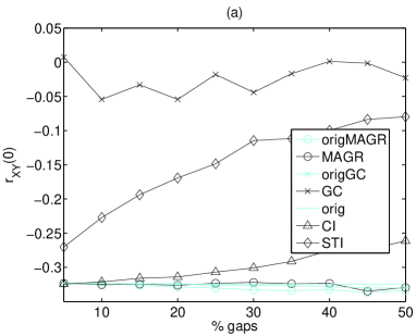
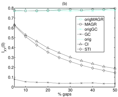
Figure 1: Zero lag cross correlation for the MVAR system in (a) and zero lag cross mutual information for the coupled Henon map in (b) as a function of the percentage of gaps in time series of length $N=500$, using MAGR, gap closure (GC), cubic interpolation (CI) and stochastic interpolation (STI). Superimposed are also shown the estimates for time series without gaps of appropriate matching length for each gap treating method (denoted by ’orig’ in the legend).

Gap-closure (GC) performs worst, giving $r_{XY}(0)$ at the zero level for any $g$, because even if there is a single gap in the time series, after gap closing the subsequent sample pairs are not matched. This failure of GC is constantly observed in all the simulations. On the other hand, MAGR stays at the level of the original $r_{XY}(0)$ for any $g$, up to 50% of $N$ that we have tested. The same applies for cross mutual information. An illustrative example is shown in Fig. 1b for $I_{XY}(0)$ and the coupled Henon system. The only notable difference to Fig. 1a, is that CI and STI follow the same pattern of decrease of $I_{XY}(0)$ towards the zero level with $g$.

The effectiveness of gap treating techniques can be better expressed by the performance of d$r$ or d$I$ that should optimally be at the zero level. In Fig. 2, d$r$ and d$I$ are shown for the same experimental setup as for Fig. 1, adding also the results for three other gap-filling methods.

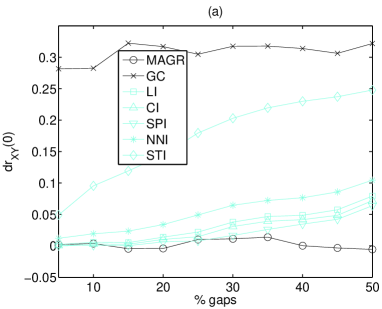
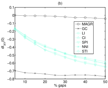
Figure 2: Difference in the zero lag cross correlation, d$r_{XY}(0)$, for the MVAR system in (a) and zero lag cross mutual information, d$I_{XY}(0)$, for the coupled Henon map in (b) as a function of the percentage of gaps in time series of length $N=500$, for the gap-treating techniques as shown in the legend.

The bound of worst performance is set by GC giving the largest difference d$r$ or d$I$ (the correlation estimate of the gap-closured time series is at the zero level), while MAGR actually lies at the bound of best performance, giving d$r$ or d$I$ at the zero level (the correlation estimate does not change after applying MAGR). In-between these two bounds lies the performance of the gap-filling techniques at a varying order but following the same pattern of d$r$ or d$I$ deviating from zero with $g$. For the linear system in Fig. 2a, all but STI gap-filling techniques perform quite adequately for small $g$ and gradually worsen for larger $g$. STI performs worse, possibly because it fills the gaps essentially with random numbers, while the other gap-filling techniques assume some simple relationship of the edge points of the gaps that here seems to be better than random. This seems to work satisfactorily when there are few gaps in the time series, say up to 25% of $N$ for the linear system. However, when the structure of the time series is nonlinear, all gap-filling techniques fail in the same way, as shown in Fig. 2b.

4.3 Transfer entropy estimation

The performance of the gap treating techniques for increasing number of gaps in the time series when using transfer entropy (TE) is similar to that for the correlation measures in Sec. 4.2. TE is a more complicated measure than the correlation measures as it involves the probability distribution of reconstructed points at higher dimensions, and it is therefore more data demanding. In order to obtain sensible TE estimates we use in the simulations time series of length $N=1500$. In Fig. 3, the results on dTE_X→Y are shown for the MVAR and coupled Henon systems and for the two smallest embedding dimensions, $m=1$ and $m=2$.

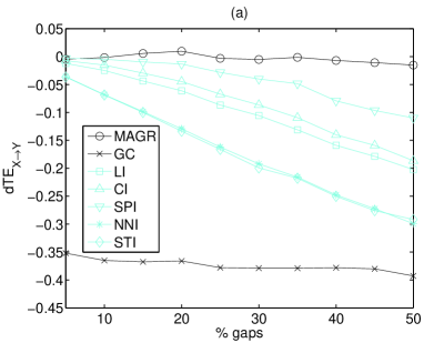
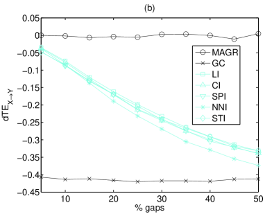
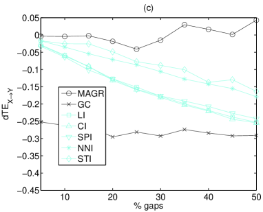
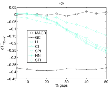
Figure 3: Difference in the transfer entropy dTE_X→Y as a function of the percentage of gaps in time series of length $N=1500$, for the gap-treating techniques as shown in the legend. (a) MVAR system and $m=1$, (b) coupled Henon map and $m=1$, (c) MVAR system and $m=2$, (d) coupled Henon map and $m=2$.

Again MAGR gives dTE at the zero level for any $g$ up to 50% of $N$. Gap-filling techniques achieve this only for very small $g$, and as $g$ increases dTE approaches the largest in magnitude dTE obtained by GC (for any $g$). This pattern holds for both the linear and the nonlinear system and for $m=1$ and $m=2$. For the coupled Henon map and $m=2$ (Fig. 3d), the gap-filling techniques improve the TE estimation for small $g$ and all but SPI give dTE at the zero level. A possible explanation for this is that for the Henon system the information of the one missing sample is partially compensated by the next existing sample, as the individual dynamics are two dimensional.

We stress here that the reported results are for the mean dTE over 50 realizations. Though MAGR gives mean dTE at the zero level the variance of dTE increases with the number of gaps because the effective number of data points is reduced (see Fig. 4).

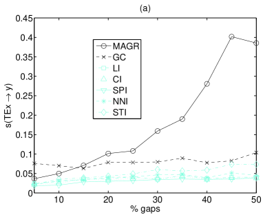
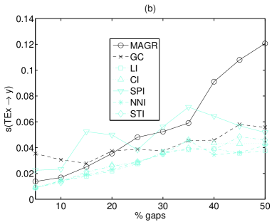
Figure 4: Standard deviation of the transfer entropy TE_X→Y, $s(\mbox{TE}_{X\rightarrow Y})$, as a function of the percentage of gaps in time series of length $N=1500$, for the gap-treating techniques as shown in the legend. (a) MVAR system and $m=2$, (b) coupled Henon map and $m=2$.

For example, for $m=2$, $N=1500$ and $g=750$, the joint data matrix of $(y_{t+1},x_{t},x_{t-1},y_{t},y_{t-1})$ is drastically reduced from 1498 to less than 150 points left to compute the correlation sums in (6). For the MVAR system the estimation variance is not affected by the gap percentage for all but MAGR methods, whereas for MAGR it increases steadily with the gap percentage (Fig. 4a). For the coupled Henon maps, the increase of the standard deviation of TE with MAGR is smaller than for the MVAR system (Fig. 4b). Moreover, for the coupled Henon map, the standard deviation of TE increases with the gap percentage up to 35% for the other methods as well at a similar rate to MAGR, and then stabilizes, whereas for MAGR it continues to increase. It seems that the increase of the variance of the TE estimation with the gap percentage varies with the underlying system and method parameters. A possible remedy for stabilizing the TE estimation would be to use larger $r$ for smaller time series (in the simulations $r$ is fixed to 0.2). We do not consider this as a drawback of MAGR but merely as an indication of the insufficiency of TE estimation when there are far too many gaps in the time series, especially when $m$ gets large. In fact, using any of the gap-filling techniques the TE estimation has the same variance as for the original time series irrespective of $g$, but always fails to match the expected TE as if there were no gaps, and the deviation of dTE increases with $g$.

4.4 The effect of time series length

In the simulations above we fixed the length $N$ of the generated time series and varied the number of gaps in it in order to assess the dependence of the performance of the gap treating techniques on the density of gaps. Here we want to examine the dependence on $N$, and therefore we fix the percentage of gaps to 20% and to 40%, and vary $N$ from 500 to 2500. We concentrate on TE as it is the most data demanding of the three studied measures and also set $m=2$. The results for the coupled Henon map are shown in Fig. 5.

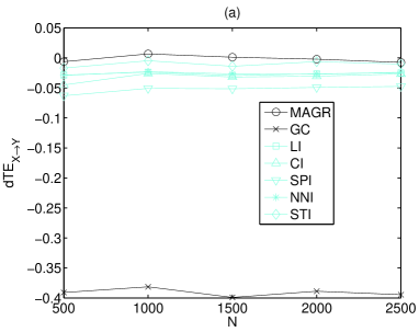
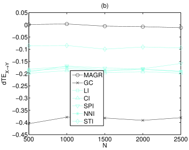
Figure 5: The dependence of dTE_X→Y ($m=2$) for the gap treating methods, as shown in the legend, on the length $N$ of the time series generated by the coupled Henon map. The percentage of gaps is 20% in (a) and 40% in (b).

Similar were the results for the MVAR system (not shown). It is clear that all methods are stable with respect to $N$ giving the same dTE for the whole range of tested $N$. Again dTE obtained by GC gives the bound of worst performance, while MAGR performs best attaining always dTE at the zero level. On the other hand, the gap-filling methods give dTE close to zero (but larger in magnitude than the dTE from MAGR) for low gap percentage (Fig. 5a), but for larger gap percentage dTE deviates away from zero (Fig. 5b).

4.5 The effect of block gaps

In real time series, there may be consecutive missing values termed block gap. Here, we examine how the gap treating techniques cope with the presence of block gaps in the time series. We consider both fixed size blocks and varying size blocks. To generate time series with block gaps, we remove block of elements of a given size from the time series so that the final number of missing values is $g$. Also we apply the restriction of not having connected or overlapping block gaps.

4.5.1 Fixed size block gaps

The results we obtained for block gaps of fixed size were essentially the same as for the single gaps. Again the two bounds of performance were set by GC, giving the largest deviation of the connectivity measure from the measure on the non-gappy time series, and MAGR, giving good matching of the connectivity measure on the gappy and non-gappy time series. The gap-filling techniques exhibited again a deviation increasing with the number of block gaps. The only difference as compared to the case of single gaps is that STI was significantly improved, giving much less deviation than the other gap-filling methods.

In Fig. 6, the results of the simulations are shown for the coupled Henon map, $N=1500$, and TE estimation for $m=1$ and $m=2$ using block gaps of size 5 and 10.

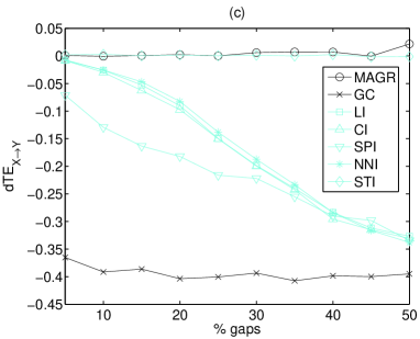
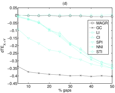
Figure 6: Difference in the transfer entropy dTE_X→Y as a function of the percentage of gaps in time series of length $N=1500$ from the coupled Henon map for the gap-treating techniques as shown in the legend. (a) $m=1$ and block gaps of size 5, (b) $m=1$ and block gaps of size 10, (c) $m=2$ and block gaps of size 5, (d) $m=2$ and block gaps of size 10.

The results confirm the performance of GC and MAGR as discussed above and show that STI distinguishes from the other four gap-filling methods. In particular for $m=1$, dTE obtained by STI has the smallest deviation from the zero level over all gap-filling methods, increasing also with $g$, but slower when the size of the block gaps gets larger, while the other gap-filling methods do not seem to be affected by the size of the block gap. For $m=2$, STI improves further and dTE stays at the zero level as for MAGR. A possible explanation for this is that because STI does not make any assumption on the underlying dynamics and fills the gaps in a stochastic manner, it turns out to be more suitable when many consecutive values are missing than assuming deterministic dynamics as done by the other gap-filling methods.

With regard to the variance of the TE estimation when using MAGR, we note that the increase of variance with $g$ is much slower in the case of fixed size block gaps because fewer points of the full joint data matrix are dropped than when the gaps are of single type. For example for the setup of Fig. 6d, for $g=750$ the number of points in the joint data matrix falls from 1498 to about 350 points after applying MAGR, to be compared to 150 points for single gaps. This has a direct effect on the standard deviation of TE estimation obtained with MAGR in the 50 realizations, e.g. for $g=750$ this is 0.05 for block size 10, which is much smaller than for single gaps.

4.5.2 Varying size block gaps

We relaxed the constrain of the fixed size of the block gap and allowed for variable block gap size ranging from 1 to 15, drawn randomly, i.e. from a discrete uniform distribution in the range 1 to 15. As before, when generating the gappy time series the restriction of not having consecutive or overlapping block gaps was applied, and blocks were added until the predefined gap percentage was reached.

The results follow a similar pattern as in the case of the block gaps of fixed size, as shown in Fig. 7 on the same experimental setting for $m=1$ and $m=2$.

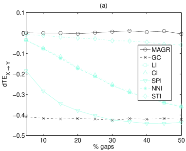
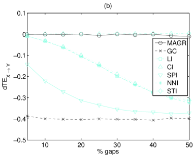
Figure 7: Difference in the transfer entropy dTE_X→Y as a function of the percentage of varying size gaps in time series of length $N=1500$ from the coupled Henon map, for the gap-treating techniques as shown in the legend. (a) $m=1$ and (b) $m=2$.

The best performing method is MAGR with second best STI, which deviates from dTE’s zero level slowly with the gap percentage for $m=1$ but stays at the zero level as MAGR for $m=2$. The performance of the other methods is inferior with GC being for all gap percentages at the same large deviation and the rest declining towards this with the gap percentage. Interestingly, for $m=1$ the CI method approaches and even exceeds for large gap percentage the lower bound of GC.

5 Application

Here we assess MAGR in conjunction with the correlation and causality measures on financial time series. We used daily data of five European stock market indexes from 13 October 2008 to 8 September 2011. The selected period covers the financial crisis starting at about September 2008 as well as the sovereign debt crisis of 2010-2011, including turbulent as well as less turbulent periods. Moreover, we observed in this period the least occurrences of gaps with a rate of 2.6% to 3.7% of the data, which is much lower than for other past periods. Also, the length of the selected period is adequately large for the estimation of the connectivity measures when we artificially insert gaps.

The stock markets selected include big and medium economies, countries that experienced the financial turmoil in different degrees of severity and also countries that share a common currency as well as others that they have their own. The final sample consists of the stock market of France (FCHI), Germany (GDAXI), Netherlands (AEX), Spain (IBEX35) and Switzerland (SSMI). The historical close index prices are shown in Fig. 8a and their returns (log differences) in Fig. 8b.

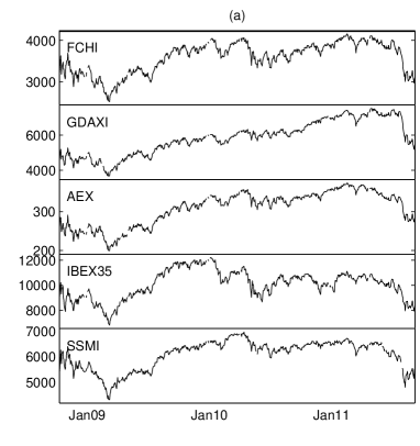
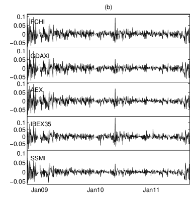
Figure 8: (a) The close index of 5 financial markets, as indicated in the panels, in the period 13 Oct 2008 to 8 Sep 2011. (b) The returns of the indexes in (a).

Despite the increased volatility in the starting period we consider the returns time series of the five markets as fairly stationary and proceed with the analysis on them.

The analysis consists of the estimation of cross correlation, cross mutual information and TE on the original time series and the time series added with random gaps. The latter were constructed by inserting blocks of gaps of random size (ranging from 1 to 5) into the original time series thus achieving an overall level of missing values of 10% and 20%.

The estimated cross correlation and cross mutual information for the gappy time series using MAGR is very close to the respective values obtained on the original time series, as shown in Fig. 9.

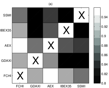
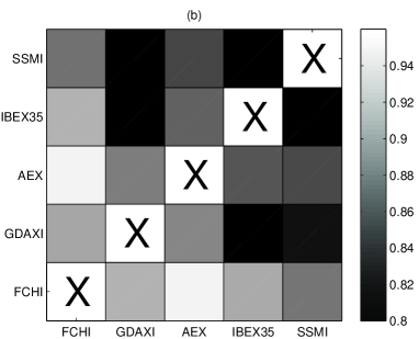
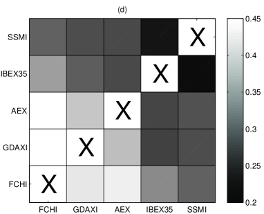
Figure 9: Color maps at grey scale of the correlation measures on the original time series of the six financial indexes at the lower-right triangular part and the gappy time series (using MAGR) at the upper-left triangular part. (a) cross-correlation and 10% gaps, (b) cross-correlation and 20% gaps, (c) mutual information and 10% gaps, (d) mutual information and 20% gaps.

For each of the panels in Fig. 9, each cell of the upper-left triangular part for the gappy time series has the same gray-scale color as the symmetric cell in the lower-right triangular part for the original time series, indicating that for each pair of financial indexes the correlation measure has approximately the same value when computed on the original and gappy time series. The only slight deviation that can be observed is for the cross mutual information when the percentage of gaps is 20% (see the pair GDAXI - IBEX35 in Fig. 9d). Thus the correlation between the financial indices could be reliably estimated even if a good number of values were missing. The results show that AEX, FCHI and GDAXI correlate stronger to each other than IBEX35 and SSMI. It is noted that the estimation of the correlation measures was stable with respect to the gaps inserted though the length of the gappy time series was reduced from about 735 to 640 for 10% gaps and to 490 for 20%, depending on the financial indexes. Actually, for the pair GDAXI - IBEX35 the cross mutual information gave somehow larger value for 20% gaps (from 0.265 to 0.293), the length of the gappy time series was the smallest being 474.

Regarding the transfer entropy, its values on the gappy time series using MAGR deviate more from the original financial time series, as shown in Fig. 10.

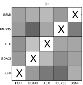
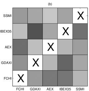
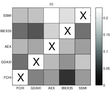
Figure 10: Color maps at grey scale of the transfer entropy on the six financial indexes: (a) original time series, (b) time series with 10% gaps, and (c) time series with 20% gaps. The driving effect is from row to column.

Adding 10% gaps does not change significantly the estimation of TE, and although there are small changes in the TE values, the overall pattern of causal relationships remains essentially the same. Still, there is no systematic bias and the deviations are randomly positive and negative. For 20%, the original pattern of causal relationships is retained relatively well but there are substantial differences, visible in the color maps, i.e. comparing Fig. 10a to Fig. 10c. Though the variance increases with the gap percentage there is no bias and the TE value decreases, e.g. from FCHI to IBEX35, and increases, e.g. from SSMI to AEX, in a random manner. The reason for having for 20% gap percentage larger variance in the TE estimation than in the correlation estimation is that TE is more data demanding. Indeed for the simplest setup of TE used here ($m=1$, $\tau=1$) the effective number of data points is only slightly smaller than for the correlation measures, and specifically the number of data points for the original time series is about 725 and decreases to 620 for 10% gaps and to 460 for 20%, depending on the financial indexes.

6 Discussion

We have presented a simple idea for treating the gaps in multivariate time series when computing a connectivity measure, such as the cross correlation, cross mutual information and transfer entropy. The considered connectivity measures suppose a joint data matrix, where the rows are time ordered and each row regards a vector of present, and possibly past and future observations of both variables. The idea is to omit the rows that contain empty entries, corresponding to missing values, and proceed with the calculations on the matrix of reduced rows. The important advantage of this approach, called measure adapted gap removal (MAGR), is that the dynamics of the (possibly) coupled system is intact, which is in contrast to all the gap-filling methods, replacing the gaps under a stochastic or deterministic model for the underlying dynamics. Certainly, any hypothesized model cannot be appropriate for every problem. Our simulations on a linear and a nonlinear coupled system revealed the inadequacy of the gap-filling methods (we considered linear, cubic, spline, nearest neighbor and stochastic interpolation), and confirmed the appropriateness of MAGR, in estimating connectivity measures in bivariate time series with gaps.

An apparent disadvantage of MAGR is that the amount of available data for the computation of the connectivity measure is reduced at a degree that depends on the number of gaps $g$ in conjunction with the type of gaps (the same $g$ can regard many single missing values or few groups of consecutive missing values called block gaps), and the parameters of the connectivity measure, e.g. the embedding dimension $m$ in the measure of transfer entropy. Thus using MAGR in a setting involving, say, a large $g$ and $m$, there may be insufficient data points to compute the connectivity measure and the estimate may have large variance. Actually, this is equivalent of having an equally small non-gappy time series, and the simulations showed indeed the good matching of the two estimates of the connectivity measure, on the gappy time series treated by MAGR and the non-gappy time series of equivalent length. The simulations showed that MAGR gives no deviation of the average connectivity measure estimated on the gappy and non-gappy time series, irrespective of $g$, but the estimate may have larger variance (implied by the amount of available data), whereas the gap-filling methods give deviation that increases with $g$. The worst performance was observed for the gap closure method, which is actually based on the strongest, and generally least valid, assumption of independent observations. Thus for time series with many gaps, the estimate of a connectivity measure using a gap-filling method will tend to deviate, whereas using MAGR it will be at the level of the estimation on the time series of reduced length.

We also found that when the same number of gaps occur in blocks of fixed or varying size, it makes no difference for the performance of the gap-filling methods, except for the stochastic interpolation, which improved with the size of the block gap. On the other hand, for MAGR the estimation is equally well matched but now the variance is decreased as the rows of empty entries in the joint data matrix is reduced. The latter does not regard measures that involve only present values in the rows of the joint data matrix, such as the zero lag cross correlation and cross mutual information, for which the data reduction in MAGR is the same for single and block gaps.

The above findings suggest that, depending on the sensitivity of the connectivity measure estimate to the time series length, estimates on different bivariate time series of the same length but with varying amount of gaps should not be directly compared, either using a gap-filling method or MAGR. Using MAGR, the comparison should be done on the basis of joint data matrices with non-empty entries of the same size. This situation may be met in many applications using windowing of multivariate time series records where gaps of irregular size and frequency may occur, e.g. in the analysis of multi-channel electroencephalograms (EEG) or financial market indices. However, our exemplary study on a set of six financial market indices showed that MAGR can provide reliable estimates of correlation and causality measures even when there are significant gaps in the time series. Besides fluctuations in the estimation of the transfer entropy that increased with the gap percentage, the causal relationships for each pair of indexes could be robustly estimated. It is noted however, that these results were obtained with a simple setup for the transfer entropy, and increasing the embedding dimension would result in drastically decrease of the effective data size using MAGR and subsequently larger variance in the estimation of transfer entropy. Still the obtained evidence from the simulations and the application in finance shows that for small percentage of gaps or large time series MAGR is a suitable approach to obtain reliable estimates of cross-correlation and Granger causality.

In this work, we demonstrated the MAGR approach on some bivariate connectivity measures. Though MAGR is measure specific and has to be adapted to the selected measure, it is straightforward to adapt it to any measure that has as a core a joint data matrix, which encompasses most of the measures on multivariate time series. For example, MAGR can directly be applied to partial transfer entropy, conditioning the driving-response effect on other observed variables [28, 22]. Simply, the joint data matrix is expanded containing columns for the other observed variables. Certainly, if there are asynchronous gaps in the time series of the other variables, the size of the matrix will be further reduced affecting the stability of the measure estimation. The systematic analysis using multivariate causality measures is the subject of a forthcoming study. MAGR can also be applied to models of univariate and multivariate time series, as they also rely on a joint data matrix. For example, for an univariate autoregressive model, the matrix of lagged variables has the role of the joint data matrix, and after the elimination of the rows of empty entries the ordinary least squares can be applied to compute the model parameters. The extension to multivariate autoregressive models is straightforward.

References

- Bahadori and Liu [2012] Bahadori, M. T., Liu, Y., 2012. Causality analysis in irregular time series. In: SIAM International Conference on Data Mining. pp. 660–671.
- Bressler and Seth [2011] Bressler, S. L., Seth, A. K., 2011. Wiener-Granger causality: A well established methodology. NeuroImage 58, 323–329.
- Broersen [2009] Broersen, P., 2009. Practical aspects of the spectral analysis of irregularly sampled data with time-series models. Instrumentation and Measurement, IEEE Transactions on 58 (5), 1380–1388.
- Cellucci et al. [2005] Cellucci, C. J., Albano, A. M., Rapp, P. E., 2005. Statistical validation of mutual information calculations: Comparison of alternative numerical algorithms. Physical Review E 71, 066208.
- Cover and Thomas [1991] Cover, T., Thomas, J., 1991. Elements of Information Theory. John Wiley and Sons, New York.
- Dahlhaus et al. [2008] Dahlhaus, R., Kurths, J., Maas, P., Timmer, J. (Eds.), 2008. Mathematical Methods in Time Series Analysis and Digital Image Processing. Springer-Verlag, Berlin / Heidelberg.
- Dergachev et al. [2001] Dergachev, V. A., Gorban, A. N., Rossiev, A. A., Karimova, L. M., Kuandykov, E. B., Makarenko, N. G., Steier, P., 2001. The filling of gaps in geophysical time series by artificial neural networks. Radiocarbon 43 (2A, Part 1), 365–371, 17th International Radiocarbon Conference, Jerusalem, Israel.
- Elshorbagy et al. [2002] Elshorbagy, A., Simonovic, S. P., Panu, U. S., 2002. Estimation of missing streamflow data using principles of chaos theory. Journal of Hydrology 255, 123–133.
- Facchini and Mocenni [2011] Facchini, A., Mocenni, C., 2011. Filling gaps in ecological time series by means of twin surrogates. International Journal of Bifurcation and Chaos 21 (4), 1085– 1097.
- Harvey and Pierse [1984] Harvey, A. C., Pierse, R. G., 1984. Estimating missing observations in economic time series. Journal of the American Statistical Association 79 (385), 125–131.
- Hlaváčková-Schindler et al. [2007] Hlaváčková-Schindler, K., Paluš, M., Vejmelka, M., Bhattacharya, J., 2007. Causality detection based on information-theoretic approaches in time series analysis. Physics Reports 441 (1), 1–46.
- Hocke and Kampfer [2009] Hocke, K., Kampfer, N., 2009. Gap filling and noise reduction of unevenly sampled data by means of the Lomb-Scargle periodogram. Atmospheric Chemistry and Physics 9, 4197–4206.
- Kondrashov and Ghil [2006] Kondrashov, D., Ghil, M., 2006. Spatio-temporal filling of missing points in geophysical data sets. Nonlinear Processes in Geophysics 13, 151–159.
- Kondrashov et al. [2010] Kondrashov, D., Shprits, Y., Ghil, M., 2010. Gap filling of solar wind data by singular spectrum analysis. Geophysical Research Letters 37, L15101.
- Kreindler and Lumsden [2006] Kreindler, D. M., Lumsden, C. J., 2006. The effects of the irregular sample and missing data in time series analysis. Nonlinear Dynamics, Psychology, and Life Sciences 10 (2), 187–214.
- Kullmann et al. [2002] Kullmann, L., Kertész, J., Kaski, K., 2002. Time-dependent cross-correlations between different stock returns: A directed network of influence. Physical Review E 66, 026125.
- Kulp and Tracy [2009] Kulp, C. W., Tracy, E. R., 2009. The application of the transfer entropy to gappy time series. Physics Letters A 373 (14), 1261 – 1267.
- Manzan and Diks [2002] Manzan, S., Diks, C., 2002. Tests for serial independence and linearity based on correlation integrals. Studies in Nonlinear Dynamics and Econometrics 6 (2), 1005.
- Musial et al. [2011] Musial, J. P., Verstraete, M. M., Gobron, N., 2011. Comparing the effectiveness of recent algorithms to fill and smooth incomplete and noisy time series. Atmospheric Chemistry and Physics Discussions 11 (5), 14259–14308.
- Papana and Kugiumtzis [2009] Papana, A., Kugiumtzis, D., 2009. Evaluation of mutual information estimators for time series. International Journal of Bifurcation and Chaos 19 (12), 4197–4215.
- Papana et al. [2011] Papana, A., Kugiumtzis, D., Larsson, P. G., 2011. Reducing the bias of causality measures. Physical Review E 83, 036207.
- Papana et al. [2012] Papana, A., Kugiumtzis, D., Larsson, P. G., 2012. Detection of direct causal effects and application in the analysis of electroencephalograms from patients with epilepsy. International Journal of Bifurcation and Chaos 22 (9), 1250222.
- Papana et al. [2013] Papana, A., Kyrtsou, C., Kugiumtzis, D., Diks, C., 2013. Simulation study of direct causality measures in multivariate time series. Entropy 15 (7), 2635–2661.
- Paparella [2005] Paparella, F., 2005. Filling gaps in chaotic time series. Physics Letters A 346 (1-3), 47–53.
- Quian Quiroga et al. [2000] Quian Quiroga, R., Arnhold, J., Lehnertz, K., Grassberger, P., 2000. Kulback-Leibler and renormalized entropies: Applications to electroencephalograms of epilepsy patients. Physical Review E 62 (6), 8380–8386.
- Schreiber [2000] Schreiber, T., 2000. Measuring information transfer. Physical Review Letters 85 (2), 461–464.
- Ustoorikar and Deo [2008] Ustoorikar, K., Deo, M., 2008. Filling up gaps in wave data with genetic programming. Marine Structures 21 (2-3), 177–195.
- Vakorin et al. [2009] Vakorin, V. A., Krakovska, O. A., McIntosh, A. R., 2009. Confounding effects of indirect connections on causality estimation. Journal of Neuroscience Methods 184, 152–160.
- Warga [1992] Warga, A., 1992. Bond returns, liquidity, and missing data. The Journal of Financial and Quantitative Analysis 27 (4), 605–617.
- Wehling et al. [2008] Wehling, S., Simion, C., Shimojo, S., Bhattacharya, J., 2008. Assessment of connectivity patterns from multivariate time series by partial directed coherence. In: Allefeld, C., beim Graben, P., Kurths, J. (Eds.), Advanced Methods of Electrophysiological Signal Analysis and Symbol Grounding: Dynamical Systems Approaches to Language. NOVA publishers, Ch. 17, pp. 275–295.